Approximation by finitely supported measures
Texte intégral
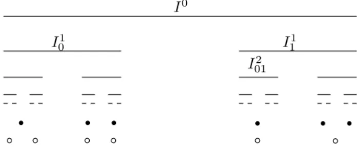
Figure

Documents relatifs
Also, W — 82 is a closed semi analytic set in C 2 of dimension at most one, and can hence be written as So u Si where So is a finite set of points and Si is a relatively
Abdollahi and Taeri proved in [3] that a finitely generated soluble group satisfies the property ( 8 k , Q ) if and only if it is a finite extension by a group in which any
holds for polynomial, i. From that it follows that every ideal in P is a principal ideal. The following are equivalent: I. J is the ideal determined by fi and
In this article, we prove a high resolution formula for the empirical measure under an averaged L p -Wasserstein metric.. Further, a Pierce type result
Abstract. We consider the problem of approximating a probability measure defined on a metric space by a measure supported on a finite number of points. More specifically we seek
This is going to imply that every quasiconvex function can be approximated locally uniformly by quasiconvex functions of polynomial growth.. The paper is organized
Such a mathematics gen- eralizes the classical Zermelo-Fraenkel mathematics, and represents an appropriate framework to work with (infinite) structures in terms of finitely
• Raise awareness of health care practitioners in primary health care (family doctors) and public health pro fessionals (including epidemiologists, hygiene specialists
