Cycle time reduction through improvements in inventory management

CYCLE TIME REDUCTION THROUGH IMPROVEMENTS IN INVENTORY MANAGEMENT by

John P. Miller

B.S., Mechanical Engineering, United States Military Academy, 1990 SUBMITTED TO THE DEPARTMENT OF MECHANICAL ENGINEERING AND

THE SLOAN SCHOOL OF MANAGEMENT

IN PARTIAL FULFILLMENT OF THE REQUIREMENTS FOR THE DEGREES OF MASTER OF SCIENCE IN MECHANICAL ENGINEERING

AND

ENG

MASTER OF BUSINESS ADMINISTRATION TSAUSN

OF TEC OLp IN CONJUNCTION WITH THE

LEADERS FOR MANUFACTURING PROGRAM AT THE

MASSACHUSETTS INSTITUTE OF TECHNOLOGY JUNE 1999

@ 1999 Massachusetts Institute of Technology, all rights reserved

Signature of Author

Department of Mechanical Engineering Sloan School of Management

May 7, 1999 Certified by

Certified by

Stanley B. Gershwin, Senior Research Scientist Thesis Advisor Arnold I.Barnett q9orgp) Eas5Van Professor of Management Thesis Advisor Accepted by

Lawrence S. Abeln Director of Master's Program Sloan School of Management Accepted by_

Ain A. Sonin Chairman, Committee on Graduate Students Department of Mechanical Engineering

CYCLE TIME REDUCTION THROUGH IMPROVEMENTS IN INVENTORY MANAGEMENT by

John P. Miller

Submitted to the Department of Mechanical Engineering and the Sloan School of Management

on May 7, 1999 in Partial Fulfillment of the

Requirements for the Degrees of

Master of Science in Mechanical Engineering and Master of Business Administration

ABSTRACT

This thesis examines a method to reduce cycle time for a product group through

improvements in inventory management. By adjusting the production sequence of orders to account for dynamics at downstream processes, inventory levels can be reduced

without jeopardizing throughput. A reduction in work in process levels can translate directly into shorter manufacturing cycle times in a flexible production environment. By reducing cycle times for existing products, the company can enhance its ability to meet customer needs.

The modified policy presented in the thesis is compared to the plant's existing policy to determine possibilities for improvement. The comparison is made using a discrete event simulation model. An experiment using the model is constructed, and the results are listed. The thesis concludes by analyzing the results and presenting recommendations for further action.

Thesis Advisors:

Stanley B. Gershwin, Senior Research Scientist

Acknowledgements

I would like to thank my advisors, Stan Gershwin and Arnie Barnett, for their guidance

and support throughout the project. I am also deeply grateful to the numerous people at the company who assisted me during my internship. Without the help and patience of Jeff, Brian, and everyone in the Industrial Engineering Group, this research would not have been possible.

I also wish to acknowledge the Leaders for Manufacturing Program for its support of this

Table of Contents

Acknowledgements ... 5

T able of C ontents ... 7

1. Introduction 1.1. Problem overview ... 9

1.2. Production system overview...11

1.3. T hesis form at ... 12

2. Background 2.1. Aluminum plate value chain ... 13

2.2. Product groupings and flowpaths ... 15

2.3. Material control policy ... 17

2.3.1. CONWIP release ... 17

2.3.2. Scheduling ... 18

2.4. Flowpath constraint dynamics ... 19

2.4.1. Heat treat and stretcher interactions ... 19

2.4.2. Problem statement ... 21 3. Solution technique 3.1. M odel overview ... 22 3.1.1. Purpose ... 22 3.1.2. Scope ... 23 3.2. System definition ... 25 3.2.1. A rrivals ... 25 3.2.2. Processing ... 26 3.2.3. Inventories ... 28 3.3. V alidation ... 29 3.4. Experiment structure ... 30

4. Results and Interpretation 4.1. W ork in process ... 32

4.2. C ycle tim e ... 33

5. Conclusions

5.1. Cycle time reduction ... 37

5.2. Transferability to other flowpaths ... 39

5.3. Implementation issues ... 39

5.4. Recommendations for further study ... 41

Appendices Appendix A: Machine utilization for Flowpath 2 ... 43

Appendix B: Parameter distributions for discrete event simulation ... 44

Appendix C: Heat treat bucket processing logic ... 45

1. Introduction

This chapter introduces the problem to be studied and provides a context for analysis.

1.1 Problem overview

In today's competitive environment, firms must be able to adequately meet customer needs quickly and cheaply. Making and delivering a product faster than rival firms has become a skill sought by many companies. To build these skills and compete on both speed and cost, many manufacturers have endorsed lean manufacturing. Lean manufacturing encourages companies to reduce the time it takes to make a product by eliminating wasteful activities and lowering excessive inventory levels.

The plant studied for this project is pursuing cycle time reduction as part of a company-wide initiative to implement lean manufacturing principles. The project was developed in close conjunction with a team formed to reduce total cycle time for all of the plant's product groups. From the team's perspective, total cycle time is defined as the time it takes for a product to travel from the first process conducted in the plant to

packaging as a final good.

Because the majority of an order's cycle time is spent waiting for processing, past efforts from similar teams have focused on reducing work in process (WIP). WIP

reduction accomplishes more than just reducing the expenses associated with holding and storing material; it also promotes lower cycle times. Cycle time, WIP, and the

throughput rate of a system are related by Little's Law, which says:

Cycle Time = WIP/ Throughput

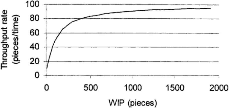
If WIP decreases, cycle time decreases as well. Unfortunately, reducing WIP can also affect throughput. WIP exists in a system as a buffer to decouple variable processes. As

the protection level of the buffer is reduced, the throughput performance of the system falls as a consequence. Figure 1.1 shows the relationship between WIP and throughput for a typical system.

100 'U ' 80 I 60 S40 0 0 500 1000 1500 2000 WIP (pieces)

Figure 1.1: WIP vs. throughput for a typical system

The plant examined in this thesis has historically operated on the right-hand side of the curve, which suggests that inventory in the system could be safely reduced. Inventory reduction in such a case would translate into faster cycle times with little impact on throughput. Now, however, the plant has reduced excess WIP in the system and must examine the current policies that govern inventory management. By improving inventory management and adjusting current policies for material release, the plant may be able to further reduce cycle times. The analysis documented in this thesis examines such an adjustment.

1.2 Production system overview

Managers in a manufacturing facility have several options available when choosing a method for controlling material flow through the plant. Proponents of lean manufacturing advocate the use of a pull system for most production environments. A pull system authorizes the release of work into the system based on system status. Work is available for processing when a change in WIP status generates a signal to release another unit of production. The signal usually corresponds to a decrease of WIP in the system at some point in the line. Such a system contrasts with a push system, which relies on scheduled work releases. Release times in a push system are based on expected demand, and orders are authorized for production according to a specified time.

Several types of pull systems can be implemented based on the production environment and company preferences. One method that works particularly well in an environment with fluctuating demand is the CONWIP system presented by Spearman, Woodruff, and Hopp (1990). CONWIP, which stands for Constant Work in Process, limits the total amount of WIP allowed in a system at any given time. When one piece is processed by the last machine in the line and exits the system, another piece is authorized

for release to the first process. The limit imposed on the line is typically measured in pieces, but it can also be measured using other means such as pounds of material. A CONWIP system can be particularly effective in a complex environment because it uses a simple mechanism to limit WIP and realize the benefits of a pull system.

A pull framework can also be implemented through use of a Kanban system. In a

Kanban system, production by a downstream machine sends an authorization signal to the machine immediately upstream. Separate WIP caps are usually maintained for each

buffer between successive processes. Such a system shows improved performance over a typical push system. CONWIP systems, however, exhibit better performance over classic Kanban in most environments as shown by Spearman and Hopp (1996).

1.3 Thesis format

This thesis examines the operations of a large aluminum rolling mill and recommends a method for reducing cycle time by modifying current policies on inventory management.

Chapter 2 describes the plant and the production practices currently employed. It gives an overview of the processes used to make aluminum and discusses the key

interactions that warrant analysis.

Chapter 3 describes the method used to analyze the identified problem. The model used is defined in terms of actual system events. Also, the experiment structure used to compare the existing system with alternative configurations is defined in this

chapter.

Chapter 4 provides results found by using the selected methodology. The hypothesis developed in previous chapters is tested, and the results are listed.

Chapter 5 presents conclusions derived from the analysis and the results. The chapter ends with recommendations for further study that the plant may adopt.

2. Background

This chapter describes plant operations and presents the plant's existing material control policy. The problem analyzed in the paper is stated at the end of the chapter.

2.1 Aluminum plate value chain

The aluminum bars used by the plant to make alloy plate products start elsewhere as bauxite ore. Large quantities of bauxite ore are mined from the ground and refined through a chemical process into alumina powder. After refinement, the alumina is

smelted into aluminum using large amounts of electricity. The molten aluminum is then cast into aluminum bars. It takes approximately four tons of bauxite ore to yield one ton

of raw aluminum.

Aluminum first arrives at the plant in the form of aluminum bars. The incoming aluminum is combined with other metals to provide the many alloys needed for the final product. Through a heat-intensive process, the metals are mixed together in large

furnaces and cast into ingot form. The ingots are then matched to an order and sent to the hot line. At the hot line, the top and bottom surfaces of the ingot are scalped off to

remove impurities. The scalped ingots are then heated in large furnaces and rolled into plates of the correct gage, or thickness.

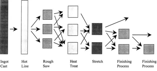
After hot rolling, the plates are set aside for cooling and cut to an approximate size for further processing. The plates must undergo several finishing processes to provide the correct size and material properties listed in the order specifications. Heat treating, stretching, and ultrasonic inspections are common processes necessary to

produce aluminum plate to meet customer needs. Figure 2.1 depicts the generic production sequence for heat treated plate products within the plant.

Ingot Cast

/1

Figure 2.1: Generic heat treated plate processing sequence

The plant is mainly organized by function and provides a job shop production environment. Pieces finishing a process are routed to the next operation where they are queued until a machine becomes available. As indicated in Figure 2.1, different products require different sequences of processes. The figure also shows that the downstream processes can be accomplished by one of several machines, each with its own

capabilities. Products may often route to any available machine for a given process, but sometimes they must go to a specific machine. A particularly thick piece, for instance , can not be stretched by a small stretcher machine and must be sent to a machine capable of handling thick pieces.

N&I

2.2 Product groupings and flowpaths

In an effort to better manage production and create a common language, management has organized the thousands of products made in the plant into fewer than fifty groups, called flowpaths. These flowpaths function as virtual transfer lines and provide a

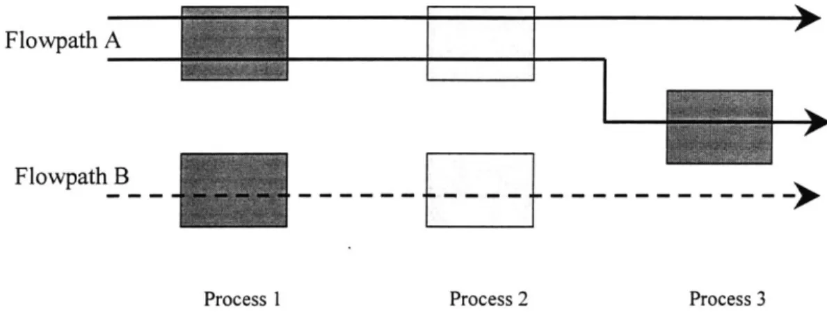
framework for manufacturing analysis in the absence of dedicated resources and physical proximity between machines. Products are organized into flowpaths based upon the processes necessary for their completion. For example, all plate products requiring heat treating, ultrasonic inspection, and milling would be placed into a single flowpath group. This group would remain separate from those products that did not require all three processes or products that required some different processes. Figure 2.2 shows an example of how flow paths are determined in the plant.

Flowpath A

Flowpath B

Process 1 Process 2 Process 3

Figure 2.2: Process-based flowpaths

Examining the three distinct paths in Figure 2.2 shows that the specific machines visited by a product do not determine its flow path. Instead, it is the sequence of

processes for a given product that determine the flowpath grouping. Even though a product traveling along the top arrow visits different machines than a second product traveling along the middle arrow, the products are grouped into the same flowpath because their process sequence is the same. The third product, which travels along the path depicted by the bottom arrow, is grouped into a separate flowpath because it is the only product that visits Process 3.

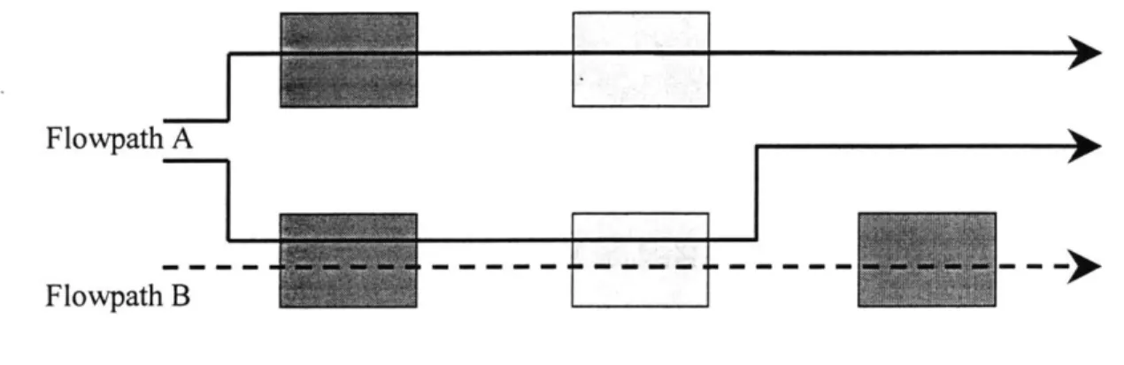
This method is quite different from the grouping seen in Figure 2.3. Here, products are organized into flowpaths according to the specific machines visited by a product. Flowpaths are separate and do not share resources.

Flowpath A

Flowpath B

Process 1 Process 2 Process 3

Figure 2.3: Machine-based flowpaths

The plant uses the method depicted in Figure 2.2 because it provides a good balance between product end uses, marketing categories, and plant capabilities. The second method, used in Figure 2.3, would allow machines to be dedicated to a flowpath and might simplify manufacturing analysis. Because machines for a given process have different capabilities, however, this method would make it difficult to apply market

forecasts and plan capacity for the plant. One of the saws in Process 2, for instance, may be able to accommodate metal that is much longer than the other saws. As a result, long pieces representing many different types of products must flow through that specific machine. Categorizing the many different types of products together and separating them

by arbitrary classifications such as alloy, length, and gage would cause undue difficulty

among business functions.

2.3 Material control policy 2.3.1 CONWIP Release

The release of metal from the ingot plant into the mill is accomplished by using a Constant Work in Process (CONWIP) system. Flowpath managers track WIP for a given flowpath and, based on throughput for the previous time period, request release of a corresponding amount of metal into the system during the next time period. For many

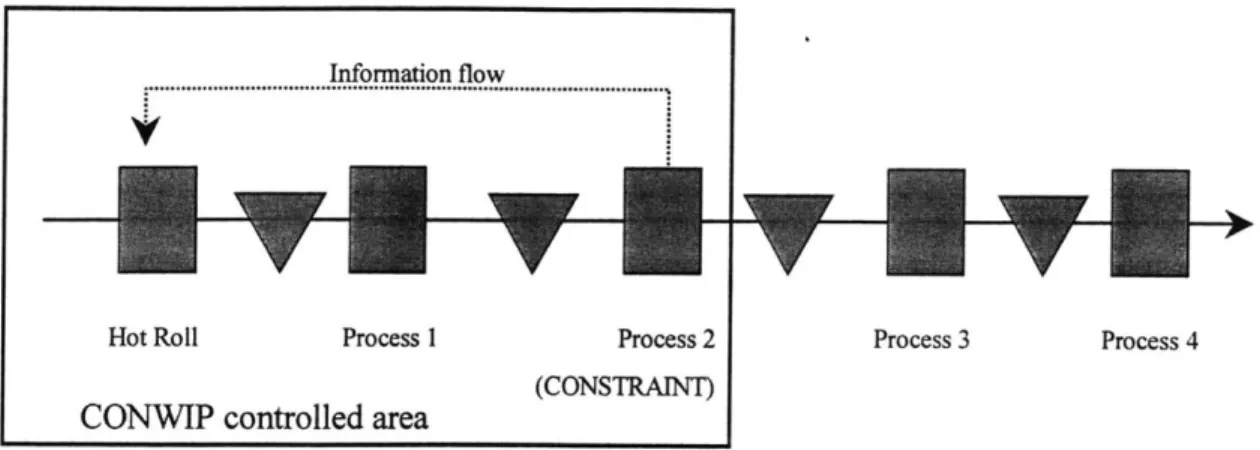
flowpaths, WIP is currently managed only between the beginning of production and the constraining process. Managers assume that once a piece travels through the constraining process, it will flow freely and WIP will not accumulate. Figure 2.4 shows the type of CONWIP loop used in the plant. The amount of metal in the system between the Hot Roll and Process 2 is monitored and is not allowed to exceed a predetermined level. As the constraining process (Process 2) completes a job, a corresponding amount of metal is introduced into the line. Each flowpath has its own CONWIP limit, even though flowpaths share nearly all resources.

Hot Roll Process I Process 2 Process 3 Process 4 (CONSTRAINT)

CONWIP controlled area

Figure 2.4: Production line with CONWIP control

2.3.2 Scheduling

When the constraining process for a flowpath completes a piece, a given quantity of metal is authorized for release into the system. For the make-to-order products, someone must then decide which orders will be filled next so that the corresponding ingots will be released to the hot line for production. This decision is made by the hot line scheduling group, which examines all outstanding orders. The group compares the expected processing time for each order with the time left until it is due, and ranks orders according to which ones must begin soonest to complete on time. In an ideal

manufacturing environment, this ranking would be followed exactly. There are many other considerations that impact the decision, however. Process peculiarities, capacity limitations, and product specifications all affect the scheduling sequence of ingots at the hot line. As a result, the scheduling group must balance a host of constraints to achieve a feasible sequencing through the hot line. Once a feasible sequence is attained, orders are broken up into lots to begin processing.

After the metal has been hot rolled, the mill schedulers take over scheduling. Mill schedulers look separately at each stage to see which lots are waiting to be processed. They then attempt to assign each lot to a specific machine after taking into account product characteristics and machine capabilities. For example, a heat treat furnace optimized to process thicker pieces of metal would be assigned the thickest pieces first. If extra capacity exists, any piece would then be assigned. Schedulers also assign an updated sequence each day for specific machine operators to follow. Again, the primary consideration for sequencing is the difference between expected times of order

completion and order due dates.

Actual production in the mill follows scheduling closely, but not exactly. Shop floor supervisors and machine operators exercise some control over which pieces they will process. On the spot decisions are made to account for broken material handling equipment or other unexpected occurrences so that production can be expedited. Also, dynamics between closely coupled machines can not be predicted and are often dealt with

by adjusting the production sequence at the shop floor level.

2.4 Flowpath constraint dynamics 2.4.1 Heat treat and stretcher interactions

The interactions between the heat treat furnaces and the stretchers are of particular interest to this project. The stretching process immediately follows heat treating for the flowpath studied and is designed to reduce the residual stresses caused by heating. Because the metal must undergo plastic deformation to relieve stress concentrations, it must be stretched before the metal ages for too long. This restriction requires that metal

can not begin heat treating until the stretcher can readily process it. In other words, the inventory that would normally accumulate in front of the stretchers must now wait in front of the heat treat furnaces so that heated metal does not age excessively before stretching.

The tight coupling of processes provides complications during this phase of manufacturing because the two processes are very different. As with many thermal processes, processing time for heat treating depends on the gage, or thickness, of the metal. Thin pieces can be heated relatively quickly, whereas thick pieces take much longer. Stretching, however, is not dependent on gage. Although the process is

theoretically dependent on alloy, cross sectional area, and final length, in practice there exists sufficient variability so that processing time appears independent of piece

characteristics. Capacity of the stretchers as compared to capacity of the heat treats then depends on the mix of thick pieces to thin pieces. When the heat treat furnaces process several batches of thick pieces, the stretchers race ahead. Conversely, the stretchers get behind when the heat treats process all thin pieces. This situation is particularly bad because of the time constraint between the processes mentioned previously. When the stretchers are full, the heat treats must stop or slow down until the backlog in front of the stretchers diminishes. If the heat treats are the constraining process for that flowpath, then lost throughput at that stage means lost throughput for the plant.

Complications also arise from differences in batches for the two processes.

Stretchers are single piece machines and have a batch size of one piece. By contrast, heat treat furnaces process the metal in batches of varying size. The number of pieces in the batch varies and is based on individual piece length and width. To complicate production

even further, each piece within a batch must be of a similar gage and of a similar alloy to the others. Although products from different flow paths can be mixed, the pieces must all be of compatible gages and alloys to ensure uniform treatment.

2.4.2 Problem statement

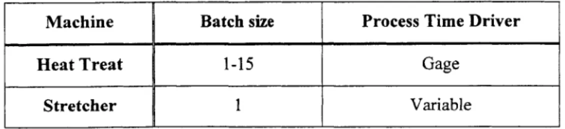
Table 2.1 summarizes the differences between the heat treating and stretching processes. To account for the process differences and the variability in production that

can ensue, the plant has historically kept large amounts of inventory in front of the heat treat furnaces. Because the operators do not know what types of pieces will enter from upstream processes, production can be jeopardized when the buffer becomes too low. By setting a CONWIP limit high enough, many different pieces of varying gage and alloy can accumulate in front of the heat treat furnaces. The accumulation provides operators there with enough flexibility to ensure full furnace utilization and meet throughput goals. However, the same accumulation of WIP brings with it increased holding costs and increased cycle time. As throughput remains relatively constant, more WIP sitting in front of the heat treats translates into more time needed for incoming metal to flow through the system. To reduce cycle time, a new way of managing inventory must be found to reduce WIP without sacrificing throughput.

Machine Batch size Process Time Driver

Heat Treat 1-15 Gage

Stretcher 1 Variable

3. Solution Technique

This section describes the solution method used to analyze the identified problem. Model formulation and experiment structure are described.

3.1 Model Overview 3.1.1 Purpose

The problem identified in the plant for further analysis concerns the long cycle times through the mill resulting from large amounts of inventory in front of the heat treat furnaces. This inventory is necessary to provide operators with the flexibility necessary to readily build batches of compatible pieces for processing. It is also important for the operators to be able to build successive batches that can run smoothly through the stretchers in single piece flow before the time restriction after heat treating elapses. Currently, lots are sequenced into the system at the hot line according to local criteria and allowed to accumulate until needed. It may be possible to improve system performance

by introducing lots into the system using a sequence that obviates the need for large

amounts of inventory in front of the heat treats. The optimized sequence could result in reduced cycle time for plate products through the entire mill.

Using discrete event simulation, an experiment can be conducted to determine whether adjusted arrival sequences from the hot line can reduce inventories and cycle times while maintaining throughput. The simulation model used for the experiment is designed to determine the average WIP, cycle time, and throughput rate for a product group given a set of material control policies. By adjusting the policies and comparing results, differences in policies can be predicted and sources of improvement identified.

3.1.2 Scope

The plant studied is renowned for its complexity. As with most complex manufacturing systems, it would be nearly impossible to model the entire plant at an exacting level of detail. To define a practical scope of study that still allows the model to accomplish its purpose, one can examine organizational structure, production data, and manufacturing practices.

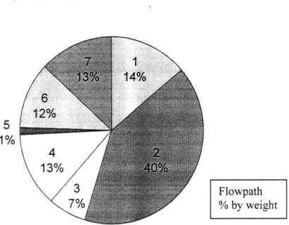
Scope can first be limited along the dimension of product groupings by using the flowpath framework that currently exists in the plant. Flowpaths for aluminum plate can be examined to identify a group of products that contribute significantly to the plant's overall production while maintaining a similar set of production practices. Upon examining plate production volumes for the plant, Flowpath 2 can be identified as a candidate for analysis. During a typical production period, the flowpath accounts for over 40% of all plate production. Figure 3.1 shows a breakdown by flowpath for plate production during a typical period.

14% 5 4 13% 3 _Flowpath 7% % by weight

Flowpath 2 can next be examined to see if it can be simplified enough for meaningful analysis. Although a flowpath is often thought of as being a relatively homogeneous group of products, the number of different process combinations within a flowpath can be ten or greater. After taking into account the different machines that may accomplish a process, it is possible for several thousand distinct paths to exist for a given flowpath. Consequently, it is important to refine selection further before attempting to model the system. During a typical production period of one month or greater, Flowpath 2 products travel through several process sequences and visit fifty different machines. By examining production data and looking for major processes and major machines, it is possible to reduce this number to one basic flowpath through twenty different machines and still account for 85% of the flowpath. Table A. 1 in Appendix A shows the

percentage breakdown of lots traveling through each machine in Flowpath 2.

After revisiting the purpose of the model and accounting for the parameters of interest, the scope of the model can next be reduced along the process dimension. Beginning analysis at the hot line is logical because of the decoupling between the ingot plant and the hot line. Ingot production follows a modified basestock policy in which ingots are stocked to meet expected demand from the hot line. Once an ingot continues production at the hot line, analysis of the flowpath becomes important.

Because the area of concern is within the CONWIP loop, and material is assumed to flow freely after the constraint, processes after stretching can be left out of the model

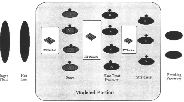
as well. Restricting the model from the hot line through the stretchers will streamline model development while allowing important characteristics to be observed. Figure 3.2

shows the scope of the model used for simulation. The model includes three major buffer locations, called buckets, and three major processes.

Igt Hot

Plat Line pFiisin

Figure 3.2: Modeled portion of Flowpath 2

3.2 System Definition

3.2.1 Arrivals

Based on arrival data over a three-month period, lots (single or multiple pieces) can be introduced into the model according to the actual sequence observed in the plant. Each piece entering the system is assigned an actual weight, gage, and alloy for the duration of the simulation. Once the three-month arrival sequence is exhausted, the simulation can repeat the sequence to provide longer simulation trials.

Pieces are released continuously into the system whenever the amount of WIP in the system drops below the CONWIP limit. As the stretcher processes metal, the amount

RS Bucket ST Bu&et

Ss

Moeld Furces

of WIP in the system drops and pieces are released from the hot line. In the current plant environment, CONWIP is synchronized with heat treat throughput. The CONWIP loop for the model, however, extends through the stretchers to simplify model construction and operation. Because the amount of metal in front of and inside the stretchers is only a small percentage of total WIP, the model can be safely simplified by extending the CONWIP loop.

3.2.2 Processing

The three major processes modeled in the simulation are rough sawing, heat treating, and stretching. Each process is broken down into the major machines visited by products in the select group from Flowpath 2. As indicated in Figure 3.1, eleven

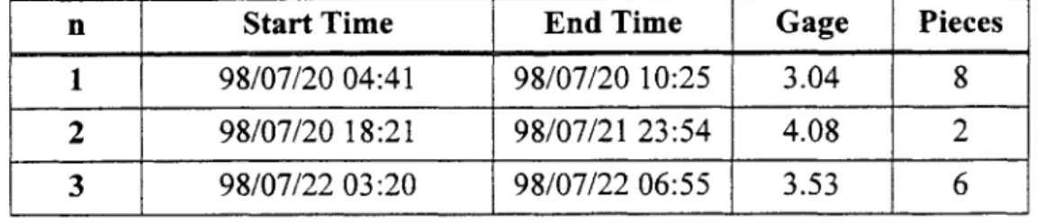
machines are modeled for the three operations. Machines within a process operate independently and have their own processing rates. Because each machine is shared by other product groups, it is necessary to also account for periods of non-availability for each machine. These periods, which include time spent producing products from other flowpaths, are modeled as operational-dependent failures. Each machine also has an expected repair period which represents time spent waiting for other product groups to be processed. Table 3.1 shows representative source data used to calculate processing times and periods of non-availability for one machine. The table shows all time blocks for which the machine was processing products in Flowpath 2. Gaps between the end time of one block and the start time of the following block indicate times when the machine was not available to Flowpath 2.

n Start Time End Time Gage Pieces 1 98/07/20 04:41 98/07/20 10:25 3.04 8 2 98/07/20 18:21 98/07/21 23:54 4.08 2 3 98/07/22 03:20 98/07/22 06:55 3.53 6

Table 3.1: Base data for processing time and non-availability

Using Table 3.1, the processing time per piece for saws and stretchers is calculated by

(EndTime n - StartTime _{) )/pieces}

For heat treating, the processing time depends on the gage of the pieces in the batch. It is measured in time units per inch and is found using

(EndTime n - StartTime ,

)/

Pieces at each machine are processed until the machine becomes unavailable to the selected product group. The amount of time is analogous to time to failure (TTF) and is found by

EndTimen - Start Timen

The time spent waiting for the machine to finish other product groups and become available to the selected group is given by

StartTimen+1 _{- EndTimen}

For each parameter, values are recorded for each piece or batch and given equal weighting.

For the least important parameters, the mean is computed and treated as deterministic, or non-random. Parameters of greater importance use exponential

distributions to introduce variability into the simulation. For the most critical processes, such as heat treating and stretching, a best-fit distribution is computed using statistical software and used in the simulation. Appendix B contains detailed statistical practices used for each machine.

3.2.3 Inventories

Because of the amount of time each piece spends waiting for processing, accurately modeling the inventories is important. For this model, there are three major inventory locations: the rough saw bucket, heat treat bucket, and stretcher bucket. Each bucket has its own peculiarities that impact system performance.

The rough saw bucket accomplishes two purposes. Like the other inventory locations, it serves as a buffer to facilitate production at the saws. It also serves as a cooling station for metal arriving from the hot line. Because of this cooling requirement, there is a random delay for incoming metal. Once the metal cools it is released to the first available saw for processing.

The modeling for the heat treat bucket is the most complex. Because the heat treat furnaces can only process batches of compatible alloys and gages, arriving pieces are segregated into bins according to their alloy group and their gage group. For

simulation purposes, there are five alloy groups and eight gage groups. Once the number of pieces in a bin reaches the required batch size, the pieces are grouped together and

routed as a batch to the first available furnace. The algorithm for grouping and routing at the heat treat bucket is listed in Appendix C.

Batches are split back into single pieces at the stretcher bucket. There the pieces are routed to the first available stretcher on a first-in, first-out basis. To ensure that pieces do not wait too long for a stretcher and age excessively, the buffer size in the model is limited to accommodate only a few pieces.

3.3 Validation

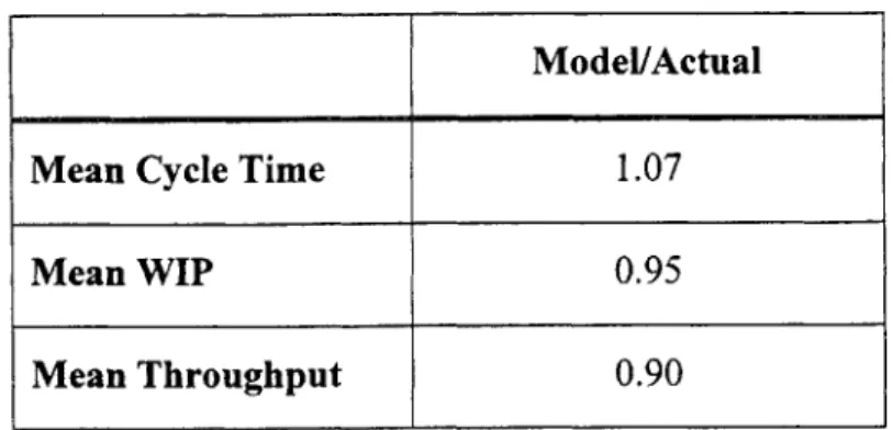
Validity of the model is examined by comparing performance of the simulation to that observed in the plant. Several important parameters can be examined to determine whether the model represents the actual environment closely enough to meet the intended purpose. Table 3.2 compares key parameters of the plant with those of the simulation. The table shows that the most important system parameters of the model are within 10% of the observed data. It should be noted that although mean values for WIP and cycle time correspond closely to those observed in the plant, the variability for these parameters in the model does not closely match that in the plant.

Table 3.2: Validation parameters

Model/Actual

Mean Cycle Time 1.07

Mean WIP 0.95

Data for the plant represents values from operations databases collected for a three-month period. Data for the simulation is found by running the simulation sixteen times with different random seeds and taking the mean of reported values. The

simulation is run each instance for a simulated time of 170 days with a 35-day period in which no data is collected.

3.4 Experiment Structure

The experiment to test whether an adjusted arrival sequence can reduce average cycle time consists of two distinct scenarios: the base case, which is designed to replicate the plant in its current condition, and the adjusted case. The adjusted case differs from the base case in that the arrival sequence of metal is changed so that pieces of similar gage and alloy are grouped together before entering the hot line. Processing logic at the heat treat bucket is also modified in the adjusted case so that pieces do not permanently accumulate while waiting for other pieces of similar alloy. This change is made to ensure that pieces from one gage grouping are completed and do not remain unprocessed for long periods of time when pieces from another gage grouping arrive. Because several flowpaths travel through the heat treat bucket and are routinely batched together, this is a reasonable assumption.

As with the validation, each trial for the experiment is run for 170

simulated days with a warm-up period of 35 days for which no data is collected. Sixteen trials are run for both the base case and for the adjusted case, and 95%

4. Results and interpretation

This section presents results obtained by using the selected methodology.

4.1 Work in process

The experiment described in section 3.4 compares system performance between the existing material control policy and one in which the arrival sequence is adjusted to account for downstream operations. For both scenarios, a desired level of throughput is maintained to account for external requirements. The first relevant comparison of system performance involves the amount of inventory in the system at a given instant. Figure 4.1 shows instantaneous WIP levels for the base case and the adjusted case during a typical simulation run.

9 8

Base Case

-Adjusted

Case

Time (Days)

Figure 4.1: Comparison of instantaneous WIP levels

Throughout the length of the simulation, the adjusted case shows significantly lower levels of WIP. Because the maximum level of inventory in the CONWIP loop can

be directly adjusted in the model, the levels seen in the figure are consistent with those expected. A run of sixteen trials for each case shows that because there is relatively little fluctuation in WIP levels among trials, the difference in average WIP levels is

statistically significant. Table 4.1 lists the 95% confidence intervals for average WIP in both cases.

Lower Bound Upper Bound

Base Case 7.33 7.36

Adjusted Case 5.16 5.19

Table 4.1: 95% confidence interval for average WIP levels

4.2 Cycle time

The cycle time for products in the two scenarios can also be compared. Let CT represent the time it takes for an average product traveling from the end of the hot line through the stretchers. Let TH represent the average throughput rate of the system for a given period. Little's Law can then be written as

CT =WIPTH

The equation shows that cycle time and WIP are proportional when throughput is held constant. As seen in Section 4.1, WIP for the adjusted case is lower than that

for the base case. Because throughput for both cases is nearly equal, it is expected that less WIP for the adjusted case corresponds to reduced cycle time for that case

as well. Simulation using the model confirms this expectation by measuring cycle time for each piece through the targeted portion of the flowpath. Figure 4.2 shows a histogram for cycle time values from a typical simulation run for each case.

6-11N40-

Adjusted

Base

Cycle Time (time periods) Figure 4.2: Histogram of cycle times

The figure shows that there are some overlapping values between cases since the longest cycle times in the adjusted case exceed the shortest cycle times in the base case. Even so, the average cycle time for the adjusted case in a typical simulation run is significantly lower. Table 4.2 shows the upper and lower bounds for a 95% confidence interval constructed from sixteen independent trials for each case.

Lower Bound Upper Bound

Base Case 101.9 104.5

Adjusted Case 73.6 74.7

4.3 Sensitivity to throughput rates

Because throughput, cycle time, and WIP are all dependent on one another, it is important to analyze the impact of changes in throughput on the other two values. To compare the two scenarios under a variety of conditions, several runs are made for each case with varying maximum allowable WIP levels. Because WIP exists to provide flexibility at the heat treat furnaces and reduce the effects of variability, it is expected that

lowering the maximum WIP in the CONWIP loop will cause a drop in throughput. For each case, the CONWIP level is set and the possible throughput recorded to indicate system performance. Figure 4.3 shows a comparison of WIP vs. throughput for both scenarios. 12 10-8 WIP +Base (units) 6 9 Adjusted 4 5 10 15 20 25 Throughput (units/time period) Figure 4.3: Throughput vs. WIP

Reducing cycle times by eradicating WIP isn't useful from a business perspective if necessary production is lost. If WIP is lowered under the base case without a change in policy, Figure 4.3 suggests that throughput will drop along the performance curve. The drop is expected since the WIP exists to provide flexibility at the heat treats and reduce the effects of variability. If the policy is changed to match that of the adjusted case, however, the results suggest that the same throughput rate can be sustained with less WIP than in the base case. The improvement in performance is most noticeable when

throughput is below 20 units/time period. Because cycle time is proportional to WIP, it is expected that the adjusted case can also deliver at most throughput rates with lower cycle times than the base case.

5. Conclusions

This section presents conclusions resulting from the analysis. It also provides recommendations for further action.

5.1 Cycle time reduction

If plant management can implement an adjusted arrival sequence similar to that

used in the simulation, cycle times can be reduced for Flowpath 2. The adjusted arrival sequence can make it possible to reduce inventory in front of the heat treat furnaces while still retaining the flexibility necessary to ensure full utilization of the heat treats. As demonstrated previously, the reduced WIP will translate into reduced average cycle time for the flowpath.

Caution should be used in determining the amount of WIP reduction possible by using an adjusted arrival sequence. Although the model replicates mean values for WIP reasonably well, WIP variability from day to day is much lower in the model than in the actual plant. Consequently, the model may indicate a higher achievable throughput rate at reduced WIP levels than what would actually be possible. This difference is caused in part by data collection methods used in the plant. WIP levels for each bucket are recorded once a day, usually at night when production is slowest and conditions are relatively stable. Throughout the day, however, differing production rates among the various machines cause actual WIP levels to fluctuate wildly. Figure 5.1 illustrates the problem by comparing the model's low-variability WIP with that of the plant.

-4 E3 Actual o : - ._ Simulation UIV .I I 0 1 21 41 61 81

Days Observed (days) Figure 5.1: WIP variability

In Figure 5.1, both the simulation and the plant have a mean WIP level of 2. The simulation WIP has relatively little variability, so it appears that WIP can be safely reduced to a mean level of 1.5 without starving downstream production processes. In the context of higher variability, however, this would not be prudent. WIP for the plant already fluctuates greatly. Reducing WIP further would cause starvation downstream and reduce throughput.

To determine the proper CONWIP limit after using an adjusted sequence, flowpath coordinators should gradually reduce the limit and observe the effects of the reduction on WIP and throughput in the mill. This method is currently employed in the plate mill and can easily be used for the adjusted sequence.

5.2 Transferability to other flowpaths

Nearly all of the resources in the plate mill, including the heat treat furnaces and stretchers, are shared among several flowpaths. Because several of the other plate flowpaths follow sequences similar to Flowpath 2, greater gains for the plant are possible if the resequencing method is also transferred to these other flowpaths. Although more

analysis is necessary, it is expected that an adjusted arrival sequence for these flowpaths could lead to further reductions in cycle times. It is also expected that the effects of a coordinated effort will be synergistic. Resources are not only shared at the machine level, they are also shared at the batch level for the heat treats since batches there may include products from several flowpaths. Because batches at the heat treats already group pieces from different flowpaths, a coordinated sequence should bring improvements in cycle time.

5.3 Implementation issues

Creating an optimal sequence for processing at the hot line is not an easy task because of the many constraints that limit the flexibility of hot line schedulers. Table 5.1 lists some of the more important constraints and their effects on scheduling. These factors make scheduling across several flowpaths a difficult problem.

Order due date Products must begin processing early enough to ship on time.

Products that require smooth surface finish Surface finish tolerance must be performed while equipment rolling

surfaces are new.

Product width Width of pieces being processed must be sequenced so that rolls wear evenly. Preheat compatibility Preheating requires batches of compatible

alloys.

Table 5.1: Hot line scheduling constraints

Implementing a system to create an optimal sequence would also be difficult in light of the current organizational structure. Although flowpath coordinators exist to speed flow along each flowpath, resources are still organized functionally. The hot line, which serves all areas of the plant, is thought of as a supplier to the plate mill. Many improvements have been made to improve the responsiveness of the hot line by reducing batch sizes and delivering pieces for the different flowpaths more often. More

coordination would be needed to enable the hot line to also supply a proper sequence of pieces that optimizes flow throughout the plant.

Plant managers have gone to great lengths to reduce cultural biases and educate operators on the importance of cycle time reduction. Even so, current processes encourage heat treat operators to concern themselves primarily with hearth utilization instead of cycle time through the downstream processes. Hearth utilization is important because the heat treats are capacity-constrained for some product mixes and limit the overall production of the line. Operators are rated in part on hearth utilization, so it is in

their best interest to retain flexibility by amassing large amounts of inventory in front of the furnace. Similarly, it is better from their point of view to build batches that ensure a

full furnace load instead of considering flow through the stretcher. If the plant chooses to implement an improved processing sequence, it will have to continue education and modify incentives to further align individual goals with those of the plant.

Care should be taken when implementing centralized planning in an environment previously characterized by operator independence. Research has suggested that some

degree of individual decision making is necessary to achieve employee commitment (Klein, 1991). When employees perceive a reduction in autonomy, negative attitudes can prevail. A shift in decision-making authority from the heat treat operators to a central

planner may alienate the operators and downplay the perceived importance of their collective expertise. Plant managers and supervisors must devise a way to implement the improved sequencing process while still providing for valuable operator input.

5.4 Recommendations for further study

With additional effort, the model used in this analysis could be developed to incorporate other flowpaths that share the same resources. The simulation model as it exists now examines one significant flowpath and its aggregate characteristics. Instead of analyzing one flowpath and projecting results onto the remainder of the plant, a more holistic model would make it possible to conduct a coordinated production study. Expanding the scope of the model slightly would also be beneficial to predict results for the entire value chain. For instance, the benefits of reducing cycle time through the heat

treats may be lost for some products if the orders simply sit downstream for a longer period of time before being shipped.

Finally, it would be of great value to extend analysis even further and investigate the plant from a total system perspective. Supply chain constraints, cultural biases, and plant organization all impact production methods used in the plant. Plant operations are also affected by the needs of other business functions such as accounting and marketing. Understanding the effects of these forces on plant dynamics and integrating them into a comprehensive analysis would be helpful in designing and implementing system

Appendix A: Machine utilization for Flowpath 2

The products grouped in Flowpath 2 follow production sequences spanning nearly fifty different workstations during normal production. To better study the flowpath and focus analysis, the least visited stations can be separated from those that are used frequently. A breakdown of machines used to produce Flowpath 2 products is listed in Table A. 1. Significant machines are shown in bold type.

Number # of lots 130 3 132 128 138 94 142 2 145 129 171 3711 181 463 186 25 190 96 192 20 - 193 -- 4 -- 1- _{94 - - --- 6} --- 2-00 -- 10 228 2 230 1 - 2 5 2 - --- 9 . 254 3484 280 11 288 1982 520 184

Number #of lots

521 3721 522 2272 523 1997 525 559 526 244 529 370 531 1246 534 1248 537 2237 538 2030 540 66 54 117 --542 TO 544 1779 546 2932 58U- -3 588 1640 608 5312 609 205 661 4471 986 5054

Appendix B: Parameter distributions for discrete event simulation

Table B. 1 lists statistical distributions and the method used to determine them for key parameters in the model. Best-fit distributions are determined by a commercial statistic package and base upon three months of recorded data.

Table B.1: Methods used for determining model parameter distributions

Model Parameter Method for determining distribution

Rough saw bucket cooling time Estimated (triangular) Rough saw processing time Non-random

Rough saw non-availability time Non-random Heat treat processing time Best-fit (Beta)

Heat treat non-availability time Estimated (exponential) Stretcher processing time Best-fit (Pearson) Stretcher non-availability time Estimated (exponential)

Appendix C: Heat treat bucket processing logic

Lots arriving to be processed by the heat treat furnaces must be grouped according to alloy and gage before processing as part of a batch. The simulation model replicates the grouping by using an iterative instruction set that executes when a piece arrives at the heat treat bucket. The algorithm interprets the specified gage and alloy code for the incoming piece and places it into the proper bin. Each bin corresponds to a specific cell in a 2-d array used by the model. When the number of pieces in the bin exceeds the current batch size, the pieces are grouped and released for further processing. The algorithm is as follows: bin[alloy,gage]=bin[alloy,gage]+ 1 int row=1 while row<=5 do begin int column=1 while column<=8 do begin if bin[row,column]>=batchsize then begin create 1 as pallet

send batchsize plate to HT2

bin[row,column]=bin[row,column]-batchsize goto LSTOP end inc column end inc row end LSTOP:

References

Bonvik, Couch, and Gershwin. A Comparison of Production-Line Control Mechanisms.

International Journal of Production Research. 1996.

Hopp, W. and Spearman, M. Factory Physics : Foundations of Manufacturing

Management. Boston, MA: The McGraw-Hill Companies, Inc., 1996.

Klein, J. A Reexamination of Autonomy in Light of New Manufacturing Practices.

Human Relations, Vol 44, No. 1. 1991.

Nahmias,S. Production and Operations Analysis, 3d ed. Chicago, IL: Irwin, 1997. Schwarzbach, P. Utilizing Rapid Modeling Technology to facilitate Lead Time

Reduction. Madison, WI: Center for Quick Response Manufacturing, 1997.

Suri, R. Quick Response Manufacturing: A Companywide Approach to Reducing Lead

Times. Portland, OR: Productivity Press, 1998.