HAL Id: hal-00905129
https://hal.archives-ouvertes.fr/hal-00905129
Submitted on 6 May 2015
HAL is a multi-disciplinary open access
archive for the deposit and dissemination of
sci-entific research documents, whether they are
pub-lished or not. The documents may come from
teaching and research institutions in France or
abroad, or from public or private research centers.
L’archive ouverte pluridisciplinaire HAL, est
destinée au dépôt et à la diffusion de documents
scientifiques de niveau recherche, publiés ou non,
émanant des établissements d’enseignement et de
recherche français ou étrangers, des laboratoires
publics ou privés.
1: Measurement techniques, uncertainties and
availability
B. Hassler, I. Petropavlovskikh, J. Staehelin, T. August, P. K. Bhartia, Cathy
Clerbaux, D. Degenstein, M. de Mazière, B. M. Dinelli, A. Dudhia, et al.
To cite this version:
B. Hassler, I. Petropavlovskikh, J. Staehelin, T. August, P. K. Bhartia, et al.. Past changes in
the vertical distribution of ozone - Part 1: Measurement techniques, uncertainties and
availabil-ity. Atmospheric Measurement Techniques, European Geosciences Union, 2014, 7 (5), pp.1395-1427.
�10.5194/amt-7-1395-2014�. �hal-00905129�
www.atmos-meas-tech.net/7/1395/2014/ doi:10.5194/amt-7-1395-2014
© Author(s) 2014. CC Attribution 3.0 License.
Past changes in the vertical distribution of ozone – Part 1:
Measurement techniques, uncertainties and availability
B. Hassler1,2, I. Petropavlovskikh1,3, J. Staehelin4, T. August5, P. K. Bhartia6, C. Clerbaux7, D. Degenstein8, M. De Mazière9, B. M. Dinelli10, A. Dudhia11, G. Dufour12, S. M. Frith13, L. Froidevaux14, S. Godin-Beekmann15, J. Granville9, N. R. P. Harris16, K. Hoppel17, D. Hubert9, Y. Kasai18, M. J. Kurylo19, E. Kyrölä20, J.-C. Lambert9, P. F. Levelt21, C. T. McElroy22, R. D. McPeters6, R. Munro5, H. Nakajima23, A. Parrish24, P. Raspollini25,
E. E. Remsberg26, K. H. Rosenlof2, A. Rozanov27, T. Sano28, Y. Sasano29, M. Shiotani28, H. G. J. Smit30, G. Stiller31, J. Tamminen20, D. W. Tarasick32, J. Urban33, R. J. van der A21, J. P. Veefkind21, C. Vigouroux9, T. von Clarmann31, C. von Savigny34, K. A. Walker35,36, M. Weber27, J. Wild37, and J. M. Zawodny26
1CIRES, University of Colorado at Boulder, Boulder, Colorado, USA 2NOAA/ESRL, Chemical Sciences Division, Boulder, Colorado, USA 3NOAA/ESRL, Global Monitoring Division, Boulder, Colorado, USA 4ETH-Zürich, Zürich, Switzerland
5EUMETSAT, Darmstadt, Germany
6NASA Goddard Space Flight Center, Greenbelt, Maryland, USA
7UPMC Univ. Paris 06, Université Versailles St-Quentin, CNRS/INSU, LATMOS-IPSL, Paris, France 8University of Saskatchewan, Saskatoon, Saskatchewan, Canada
9Belgian Institute for Space Aeronomy (IASB-BIRA), Brussels, Belgium 10ISAC-CNR, Bologna, Italy
11AOPP, Physics Department, University of Oxford, Oxford, UK
12LISA, UMR CNRS 7583, Université Paris-Est Créteil et Université Paris-Diderot, 27 Créteil, France 13Science Systems and Applications, Inc., NASA GSFC, Greenbelt, Maryland, USA
14Jet Propulsion Laboratory, California Institute of Technology, Pasadena, California, USA 15Observatoire de Versailles Saint-Quentin-en-Yvelines, Guyancourt Cedex, France 16University of Cambridge, Chemistry Department, Cambridge, UK
17Remote Sensing Division, Naval Research Laboratory, Washington, D.C., USA 18National Institute of Information and Communications Technology, Tokyo, Japan
19Universities Space Research Association, Goddard Earth Sciences, Technology, and Research, NASA Goddard Space
Flight Center, Greenbelt, Maryland, USA
20Finnish Meteorological Institute, Earth Observation, Helsinki, Finland 21Royal Netherlands Meteorological Institute (KNMI), De Bilt, the Netherlands
22Department of Earth and Space Science and Engineering (Lassonde School of Engineering), York University,
Toronto, Canada
23National Institute for Environmental Studies, Tsukuba, Japan
24Department of Astronomy, University of Massachusetts, Amherst, Massachusetts, USA
25Istituto di Fisica Applicata “N. Carrara” (IFAC) del Consiglio Nazionale delle Ricerche (CNR), Florence, Italy 26NASA Langley Research Center, Hampton, Virginia, USA
27Institute of Environmental Physics Remote Sensing (IUP/IFE), University of Bremen, Bremen, Germany 28Research Institute for Sustainable Humanosphere, Kyoto University, Kyoto, Japan
29Association of International Research Initiatives for Environmental Studies, Tokyo, Japan
30Research Centre Jülich, Institute for Energy and Climate Research: Troposphere (IEK-8), Jülich, Germany 31Karlsruhe Institute of Technology, Institute for Meteorology and Climate Research, Karlsruhe, Germany 32Environment Canada, Downsview, Ontario, Canada
34Institut für Physik, Ernst-Moritz-Arndt-Universität Greifswald, Greifswald, Germany 35Department of Physics, University of Toronto, Toronto, Ontario, Canada
36Department of Chemistry, University of Waterloo, Waterloo, Ontario, Canada
37Innovim, LLC, NOAA/NWS/NCEP/Climate Prediction Center, College Park, Maryland, USA Correspondence to: B. Hassler ([email protected])
Received: 21 October 2013 – Published in Atmos. Meas. Tech. Discuss.: 14 November 2013 Revised: 26 March 2014 – Accepted: 27 March 2014 – Published: 21 May 2014
Abstract. Peak stratospheric chlorofluorocarbon (CFC) and
other ozone depleting substance (ODS) concentrations were reached in the mid- to late 1990s. Detection and attribution of the expected recovery of the stratospheric ozone layer in an atmosphere with reduced ODSs as well as efforts to un-derstand the evolution of stratospheric ozone in the presence of increasing greenhouse gases are key current research top-ics. These require a critical examination of the ozone changes with an accurate knowledge of the spatial (geographical and vertical) and temporal ozone response. For such an exami-nation, it is vital that the quality of the measurements used be as high as possible and measurement uncertainties well quantified.
In preparation for the 2014 United Nations Environ-ment Programme (UNEP)/World Meteorological Organiza-tion (WMO) Scientific Assessment of Ozone DepleOrganiza-tion, the SPARC/IO3C/IGACO-O3/NDACC (SI2N) Initiative was
de-signed to study and document changes in the global ozone profile distribution. This requires assessing long-term ozone profile data sets in regards to measurement stability and uncertainty characteristics. The ultimate goal is to estab-lish suitability for estimating long-term ozone trends to con-tribute to ozone recovery studies. Some of the data sets have been improved as part of this initiative with updated versions now available.
This summary presents an overview of stratospheric ozone profile measurement data sets (ground and satellite based) available for ozone recovery studies. Here we document measurement techniques, spatial and temporal coverage, ver-tical resolution, native units and measurement uncertainties. In addition, the latest data versions are briefly described (in-cluding data version updates as well as detailing multiple retrievals when available for a given satellite instrument). Archive location information for each data set is also given.
1 Introduction
As man-made ozone depleting substances (ODSs) decline in the stratosphere in response to the 1987 Montreal Protocol and its subsequent amendments and adjustments, the ozone layer is expected to recover globally. A small increase in stratospheric ozone abundance over northern mid-latitudes was first reported in the 2010 WMO ozone assessment
(WMO, 2011). Although supported by a variety of ground-based, balloon-born and satellite observations, statistical analysis could not attribute this change exclusively to the de-cline of ODSs due to observational uncertainty, geophysical and dynamical variability and changes in ozone due to in-creasing greenhouse gases that cool the stratosphere. Global total ozone remained significantly lower than during the early 1980s, and surface ultraviolet radiation measurements were too variable to strongly support ozone recovery. Indications of the onset of stratospheric ozone recovery have been noted since the publication of the last ozone assessment. There are several recent publications (e.g. Maeder et al., 2010; Nair et al., 2013; Kuttippurath et al., 2013) supporting the state-ment that the second stage of ozone recovery is ongoing (as defined by the WMO, 2007, statement that “occurrence of statistically significant increases in ozone above previous minimum values due to declining equivalent effective strato-spheric chlorine”). Other publications show that ozone re-covery in Antarctica should be detectable within the next decade (Newman et al., 2006; Hassler et al., 2011). The ad-ditional four years of data available since analysis was done for the 2010 WMO ozone assessment as well as improve-ments in the homogenization of ozone data records should improve the signal-to-noise ratio in the ozone time series making trend analyses results more robust.
“SPARC Report No.1 – Trends in the vertical distribution of ozone” (SPARC, 1998) provided a comprehensive sum-mary of available data and methods for trend analysis at that time. Its main objectives were to understand the limitations of the data, to assess the consistency between various data records and create a reference database for the analysis of long-term ozone changes as a function of altitude. One of the main reasons for this approach was to avoid misinterpreting instrument drifts as actual ozone changes.
Trend analysis is made more complex by the addition of new satellite records (e.g. Aura, Envisat, Odin, and SCISAT), where each covers a shorter time period than the tradition-ally used long-term records (e.g. ozonesondes, Umkehr, li-dars, SAGE, HALOE). Adding to the problem, some of the long-term platforms have ceased taking measurements (e.g. SAGE, HALOE, instruments on Envisat), while records from other satellite platforms are difficult to combine due to drifting orbits (SBUV/2 on NOAA satellites) and different
instrument generations (e.g. moving from SBUV fixed wave-length retrievals to Aura OMI hyper-spectral retrievals). For a full long-term analysis of stratospheric ozone throughout the decline due to increases in ODSs and subsequent re-covery, multiple instrument records need to be considered. Thus, several different data sources have to be merged to al-low a complete view of past ozone changes. Recent work has shown that ozone depletion and greenhouse gas (GHG) increases impact dynamical quantities in an additive man-ner, with ozone recovery possibly cancelling atmospheric circulation effects associated with increasing GHGs. (e.g. IPCC/TEAP, 2005; McLandress et al., 2010; Polvani et al., 2011). Clearly, an understanding of atmospheric transport, circulation and wave breaking patterns is important for our understanding of ozone recovery.
The consideration of uncertainties and artifacts is crucial in ozone trend analyses, particularly when the ozone recov-ery signal is small as compared to natural geophysical vari-ability. As methods for trend and attribution analysis become more advanced, the uncertainties and instrumental artifacts buried in currently available data sets start to play a bigger role. Therefore, detailed information about measurement un-certainties, data jumps due to changes in instrumentation and drifts during long-term operation of a given instrument are essential.
There have been several attempts to produce histori-cal global ozone profile data sets; these include satellite-ozonesonde combinations starting in 1979 when the first global satellite measurements became available (e.g. Randel and Wu, 2007; Bodeker et al., 2013), global ozone data sets that extend values to 2100 using model and fitting techniques (Hassler et al., 2009; Cionni et al., 2011) for use in global climate models without stratospheric ozone chemistry and also data sets that extend the historical record backward to 1900 (Brönnimann et al., 2013). Issues of biases between in-struments, sampling, noise, gaps and differences in vertical registration (pressure or altitude) have to be addressed when creating combined data records to ensure no artificial trends are introduced.
Uncertainties in calculated ozone trends need to be re-duced. In the 2010 WMO ozone assessment, inconsisten-cies in the available ozone profile data prevented a clear overall picture of long-term ozone profile changes. A suc-cessful assessment of trends for the upcoming 2014 WMO ozone assessment requires addressing the problems of time series artifacts due to changes in instrumentation, homoge-nizing applied satellite retrievals and reducing and describ-ing measurement uncertainties. The SPARC/IO3
C/IGACO-O3/NDACC (SI2N) Initiative has brought together scientists
dealing with ground and satellite ozone profile measurements in order to consolidate efforts documenting long-term ozone profile changes. SI2N has also defined the time frame to en-sure that any data set improvements are finalized to enen-sure inclusion in the 2014 WMO ozone assessment analysis.
This paper provides a summary of the most important available ozone data sets, describes measurement methods, detection limits and uncertainty estimates, gives details about the vertical and temporal resolution of individual data sets and provides references to relevant published work. In addi-tion, improvements and homogenizations that have occurred to date are discussed. This is the first of three overview papers discussing the results from the SI2N Initiative. The second paper describes the validation of the different available ozone profile measurements (Lambert et al., 2014) and the third paper provides information about and an overview on the merging and homogenizing of different data sets and calcula-tion of long-term trends (Harris et al., 2014). Ground-based ozone profiles, ordered according to the number of available stations, are described in Sect. 2. In Sect. 3, satellite-based ozone profiles are covered. The satellite measurements are organized by measurement techniques; these include solar-/stellar-occultation measurements, limb measurements and nadir measurements. A summary, including discussion of possible temporal and spatial coverage problems for the mea-surement systems, is presented in Sect. 4.
2 Ground-based measurement systems
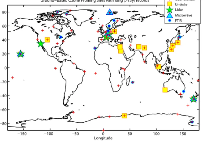
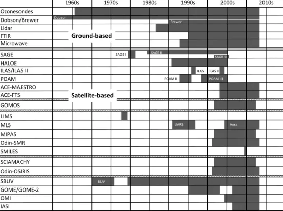
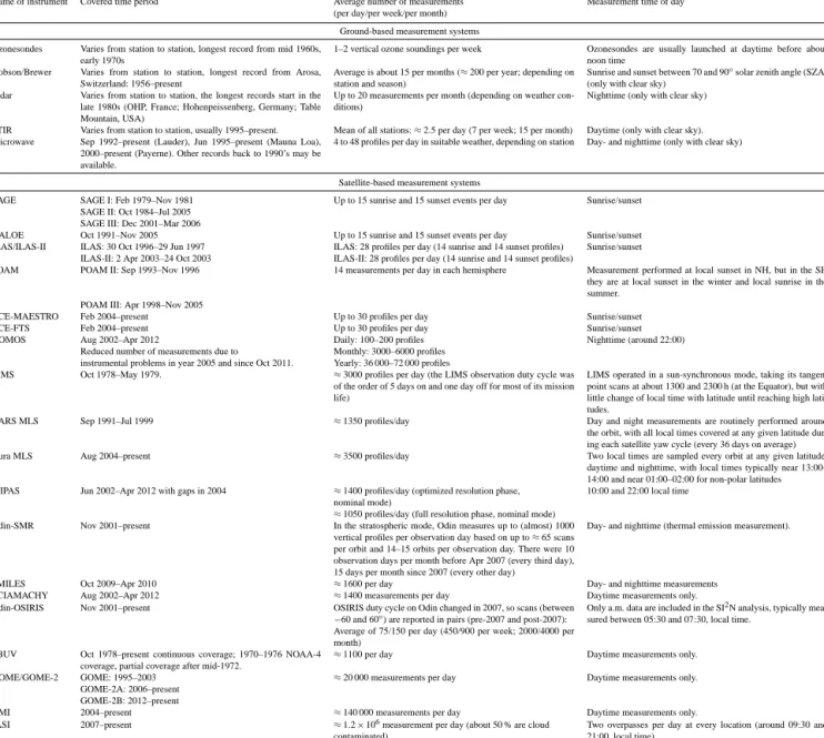
The global map with location of the ground-based instru-ment systems (ozonesonde, Dobson/Brewer, lidar, FTIR and microwave) is shown in Fig. 1. Ozonesondes and Dob-son/Brewer instruments provide the longest record of strato-spheric ozone variability (see Fig. 2). Ozonesondes are all weather sounders, and can measure at night and through clouds. Their data quality is good in the lower stratosphere and troposphere where satellites measurement quality is less reliable, and their vertical resolution is much higher than is achievable from remotely sensed measurement. Ozoneson-des are inexpensive and easily deployable. Dobson Umkehr measurements have captured evolution of the upper strato-spheric ozone prior to the satellite era and still remain the most inexpensive measurement system requiring minimal manpower. Umkehr measurements with Brewer instruments were added later, but they offer fully automated and remote-controlled operations, and furthermore add spectral UV mea-surements. Ozone lidar measurements are self-calibrated and provide high vertically resolved measurements with small uncertainties (especially for the low to mid-stratosphere). Ground-based high-resolution FTIR solar absorption mea-surements do not require an absolute calibration either; the ozone absorption lines are very narrow and are therefore self-calibrated with the reference being the surrounding con-tinuum. This technique has also the advantage of provid-ing precise total columns in addition to vertical information. Ground-based microwave measurements can be made with a time resolution of an hour or less throughout a full diur-nal cycle; their calibration is based on temperature, the mea-surements are insensitive to stratospheric aerosols, and the
−150 −100 −50 0 50 100 150 −80 −60 −40 −20 0 20 40 60 80 Longitude Latitude
Ground−based Ozone Profiling Sites with long (>15y) records Ozonesonde Lidar Microwave Umkehr FTIR
Figure 1. World map with locations of long-term ground-based
measurement sites: ozone sounding sites (red plus signs), lidar sites (green stars), microwave sites (light blue triangles), Dobson/Brewer sites with Umkehr measurements (yellow squares), and FTIR sites (dark blue circles).
instruments are nearly fully automated and require less per-sonnel time and other resources to operate than most other ground-based instruments.
2.1 Ozonesondes
Ozonesondes are small, lightweight and compact balloon-borne instruments, developed for measuring the vertical dis-tribution of atmospheric ozone up to an altitude of about 30– 35 km (see Table 1a). During flight operation, ozonesondes are coupled with standard meteorological radiosondes pro-viding temperature, pressure and wind measurements. The effective vertical resolution of the ozone profile, which is de-pendent on the balloon ascent rate, is about 100–150 m (see Table 1b and Fig. 3a).
There were 66 stations contributing data in the 2000s (Fig. 1). Ozonesonde records provide the longest time se-ries of the vertical ozone distribution throughout both tro-posphere and stratosphere; some station records start in the 1960s (see Fig. 2 and Table 1c). Most of the profiles are from the electrochemical concentration cell (ECC)-type ozonesonde (Komhyr, 1969) introduced in the early 1970s and adopted by most stations in the global network by the early 1980s. Almost all data in the most recent decade are from ECC sondes. Remaining data are from Brewer–Mast (B–M) sondes (Brewer and Milford, 1960), Japanese carbon iodine cell sondes (KC96) (Kobayashi and Toyama, 1996), and Indian sondes. Prior to the early 1990s, three stations in Eastern Europe flew the GDR (German Democratic Re-public) sonde. A majority of the data before 1980 is from B–M sondes or similar (both the GDR and Indian sondes are similar in design to the B–M sonde). All five types use the reaction of ozone with potassium iodide in an aqueous solu-tion as the method of ozone detecsolu-tion, but the instrumental
layouts are significantly different (e.g., Smit, 2002; Tarasick and Slater, 2008).
When properly prepared and handled, ECC sondes yield profiles with random errors of 3–5 % (1σ ) and overall uncer-tainties of about 5 % in the stratosphere (Kerr et al., 1994; Smit et al., 2007; Deshler et al., 2008; Liu et al., 2009). Two types of ECC sondes are in current use, with minor differ-ences in construction and some variation in recommended concentrations of the sensing solution and of its phosphate buffer. The maximum change in stratospheric response re-sulting from these systematic differences is on the order of 2–3 % (Smit et al., 2007). Other sonde types have somewhat larger random errors of 5–10 % (Kerr et al., 1994; Parrish et al., 2013).
In early intercomparisons (Attmannspacher and Dütsch, 1970, 1980), the Indian and the GDR sondes showed sig-nificantly larger random errors than other sonde types. The largest systematic differences between sondes are in the lower stratosphere, where in early intercomparisons the B– M and GDR sondes read ≈ 5–10 % lower than the ECC and KC sondes (Attmannspacher and Dütsch, 1970, 1980). The Indian sonde has generally shown little bias in the lower stratosphere, but somewhat larger random errors than the other non-ECC sondes. In later intercomparisons differences were smaller: the KC sondes were biased low by ≈ 5 % in the lower stratosphere, and the B–M sonde generally showed a small low bias as well (Kerr et al., 1994; Smit and Kley, 1998; Deshler et al., 2008).
In the middle stratosphere (below 28 km) differences in sonde response are small. As noted above, both systematic and random errors have improved with time, and from 1980 onwards (between the tropopause and 28 km) the random er-ror component of sonde measurements, for all types, is gen-erally within ±5 %, and systematic biases between them or compared to other ozone sensing techniques are smaller than
±5 % (SPARC, 1998).
Above 28 km the measurement behavior of the differ-ent sonde types is not consistdiffer-ent due to instrumdiffer-ental un-certainties (e.g. pump-flow corrections and sensing solution strength) and cannot be generally characterized. Here, B– M sondes show increasing underestimation of ozone with altitude (De Backer et al., 1998; Stübi et al., 2008), while KC sondes tend to overestimate ozone with increasing alti-tude (SPARC, 1998; Smit and Straeter, 2004; Deshler et al., 2008). In contrast, the performance of ECC sondes between 28 and 35 km is still good, overestimating ozone compared to other measurement techniques by less than 5 % (SPARC, 1998; Smit et al., 2007).
However, for ECC sondes recent studies (Johnson et al., 2002; Smit et al., 2007; Deshler et al., 2008) have demon-strated that changes of manufacturer or strength of sens-ing solution can introduce significant inhomogeneities (up to ±5–10 %) in long-term sounding records. Such artifacts, like those introduced by changes of sonde type, can be re-moved through the use of transfer functions derived from
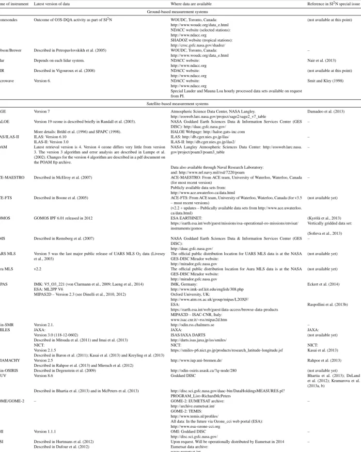
Ozonesondes Dobson/Brewer Lidar FTIR Microwave 1960s 1970s 1980s 1990s 2000s 2010s SAGE HALOE ILAS/ILAS-‐II POAM ACE-‐MAESTRO ACE-‐FTS GOMOS LIMS MLS MIPAS Odin-‐SMR SCIAMACHY Odin-‐OSIRIS SBUV GOME/GOME-‐2 OMI IASI SMILES Dobson Brewer Ground-‐based Satellite-‐based SAGE III SAGE II SAGE I
ILAS ILAS II
UARS Aura
POAM II POAM III
BUV
Figure 2. Temporal coverage of the described ground- and satellite-based measurement systems.
intercomparisons in the laboratory or field. Most station long-term records are currently being re-evaluated and ho-mogenized under the Ozonesonde Data Quality Assessment activity of the SI2N Initiative (H. G. J. Smit, personal com-munication, 2013). This should both reduce overall uncer-tainties and allow increased confidence in trends derived from ozonesonde data in future assessments.
Ozonesonde profiles are archived by the World Ozone and Ultraviolet Radiation Data Center (WOUDC), the Network for the Detection of Atmospheric Composition Change (NDACC) and the Southern Hemisphere Additional OZonesondes network (SHADOZ) (see Table 1d for more details).
2.2 Dobson/Brewer
Dobson and Brewer are ground-based spectrophotometer instruments. The Umkehr measurement is a sequence of morning or afternoon zenith-sky measurements recorded as a relative change of transmission at two spectral channels (Dobson) or photon counts at individual spectral channels (Brewer), all selected in the ultraviolet part of the zenith-sky spectrum. Measurements are taken when the sun elevation changes between 60◦and 90◦solar zenith angle (SZA), and under the assumption of static atmospheric conditions and no clouds in the zenith viewing area. The vertical resolution of an Umkehr ozone profile is ≈ 10 km. Ozone profiles (in Dobson units (DU)) are historically provided in 10 pressure
layers, where pressure at the top of the layer is half of the pressure at the bottom, while the tropospheric measurement is one thick layer below 250 hPa (see Table 1a, b). The uncer-tainty in the retrieved ozone profile is a combination of mea-surement error (increases with increasing SZA) and smooth-ing error (about 10–20 % in the troposphere and low strato-sphere and ≈ 5 % in middle and upper stratostrato-sphere).
The Umkehr record length varies by station; the longest record is from Arosa, Switzerland (starting in 1956; see Ta-ble 1c). The latest version of the ozone profile algorithm for processing of Dobson Umkehr data (UMK04) is described in Petropavlovskikh et al. (2005). Although Umkehr profiles show systematic biases in comparisons with other measure-ments (Nair et al., 2011; Kramarova et al., 2013b), this is of less concern for trend analysis when the UMK04 pro-file retrievals are used as monthly mean anomalies. However, smoothing errors, especially in the lower stratosphere, create low vertical resolution in the Umkehr retrieved profile and enhance retrieval noise in the lower stratosphere and tropo-sphere. The forward model used to process Brewer Umkehr data (O3BUmkehr v.2.6, http://www.o3soft.eu/o3bumkehr. html) was adapted from the UMK04 model taking into ac-count the different optical characteristics of the Brewer in-strument (Petropavlovskikh et al., 2011, see Table 1d).
The Umkehr method uses a technique that minimizes sys-tematic errors of instrumental drifts by normalizing to one of its measurements. Other methods are used to track instru-ment stability, such as once a month checks of wavelength
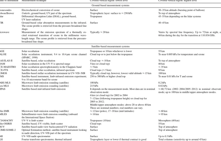
Table 1a. Summary of measurement techniques and lowest and highest covered level for the five ground-based measurement systems and all
described satellite measurement systems.
Name of instrument Measurement technique Covered vertical region: lowest level Covered vertical region: highest level Ground-based measurement systems
Ozonesondes Electrochemical conversion of ozone Surface 30–35 km altitude (bursting point of balloon)
Dobson/Brewer Umkehr, ground-based, UV part of the spectrum Tropospheric layer: surface to ≈ 250 hPa To top of atmosphere Lidar Differential Absorption Lidar (DIAL), ground-based,
UV laser radiation
Tropopause 45–55 km depending on the lidar systems
FTIR Ground-based solar absorption measurements in the infrared. The ozone profile is retrieved from the pressure-broadened line shape.
Surface 40–45 km
Microwave Measurement of the emission spectrum of a thermally ex-cited rotational transition of ozone in the millimeter wave-length range. The ozone profile is retrieved from the pressure-broadened line shape.
Typically ≈ 20 km Varies by spectral line frequency. Up to 72 km at night, and 66 km during the day for the transition at 110.836 GHz.
Satellite-based measurement systems
SAGE Solar occultation Tropopause or 10 km whichever is lower 55 km
HALOE Solar occultation instrument; 9.4 to 10.4 µm ozone channel (SPARC, 1998)
Cloud top or to just below the tropopause To near 0.005 hPa for temperature and ozone
ILAS/ILAS-II Satellite-based, solar occultation Cloud top: ≈ 10 km To top of atmosphere
POAM Solar occultation in the UV–V is spectral range 5 km (or cloud top) 60 km
ACE-MAESTRO Solar occultation spectrophotometry in the Chappuis band ≈5 km ≈35 km
ACE-FTS Satellite-based, solar occultation, infrared spectrum Cloud tops (≈ 5 km) 95 km
GOMOS Satellite-based stellar occultation instrument in UV–VIS–NIR Typically cloud top, however, lowest valid altitude ≈ 15 km 100 km LIMS Satellite-based instrument, limb-infrared emission experiment;
9 to 10 micrometer band for ozone
250 to 300 hPa or higher cloud top To near 0.01 hPa for T and ozone
UARS MLS Microwave limb emission sounding (satellite) 100 hPa 0.2 hPa
Aura MLS Microwave limb emission sounding (satellite) 215 hPa 0.02 hPa
MIPAS Satellite-based mid-infrared limb emission It depends on the measurement mode. Most data are in nominal observation mode:
≈68/72 km (2002–2004/2005–2012) in nominal observation mode; up to 100 km in middle/upper atmosphere modes. 6 km (or cloud top) for 2002 to 2004
7–12 km (following tropopause height) or cloud top for 2005 to 2012;
Middle/upper atmosphere modes: above 20 or above 40 km These are nominal numbers; real numbers can vary.
Odin-SMR Microwave limb emission sounding (satellite) ≈12 km (poles), 17–18 km (mid-latitudes) ≈60 km SMILES Submillimeter-wave limb emission sounding (onboard
the International Space Station)
≈16 km ≈95 km
SCIAMACHY UV–V is limb scatter Tropopause (10 km) Mesosphere (60 km)
Odin-OSIRIS Satellite based, UV–visible, limb scatter Cloud tops 55 km
SBUV Satellite-based nadir-view backscattered UV radiation Surface Top of atmosphere
GOME/GOME-2 Optimal Estimation method, satellite-based instrument looking in nadir direction, UV–VIS part of the spectrum
Surface Top of atmosphere
OMI UV–VIS nadir spectrometer Surface Up to 0.3 hPa
IASI Fourier transform spectrometer, thermal infrared Tropospheric layer or lower if thermal contract is good Total columns (sensitivity up to around 45 km)
registration by using standard discharge lamps, ratio of mea-surements at several spectral channels (for Brewer instru-ments, daily), and optical wedge calibration produced dur-ing Dobson intercomparisons (every 4 years). These meth-ods track degradation of the optical system. Effects of ozone cross-section values and uncertainties of stray light effects on Dobson and Brewer Umkehr ozone profiles are discussed in Petropavlovskikh et al. (2011) and WMO (2008). The re-placement of an instrument at the station can cause a step change in the Umkehr record due to the difference in the out-of-band contribution that is specific to each instrument. Thus, additional homogenization of the record may be re-quired (Zanis et al., 2006; Miyagawa et al., 2009). In addi-tion, interference from optically thick aerosol loading (vol-canic) at Umkehr spectral channels results in systematic er-rors that can be as large as 10–15 %. Therefore, about two years of data are typically removed after the Pinatubo (1991) and El Chichon (1982) volcanic eruptions. Data from 28 stations with current Umkehr measurements and of 58 sta-tions with historical Umkehr measurements are archived at WOUDC, Toronto, Canada (see Table 1d for the URL).
2.3 Lidar
Lidar (light detection and ranging) is an active, remote-sensing instrument that uses the interaction between a laser beam and atmospheric molecules and particles. Ozone lidar measurements are performed using the DIfferential Absorp-tion Lidar method (DIAL), which is based on the absorpAbsorp-tion of ultraviolet radiation by ozone and requires the emission of two laser wavelengths (so-called “on” and “off” wave-lengths) characterized by different ozone absorption cross sections (Pelon et al., 1986; Godin et al., 1989; McDermid et al., 1990). The use of pulsed lasers provides range re-solved measurements. Ozone DIAL systems include one or two lasers, depending on the technique used for the gen-eration of the off wavelength, an optical receiving system that includes a telescope for the collection of the laser light, a spectrometer or filters for the separation of the received wavelengths and an electronic data acquisition system. In the case of stratospheric ozone, photon counting is generally used for the acquisition of the lidar signal in order to provide high sensitivity and low noise. The ozone number density is commonly retrieved from the difference of the slopes of the logarithm of the lidar signals corrected for the background noise and saturation affecting large signals originating from
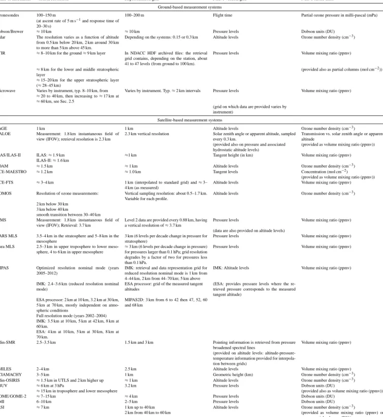
Table 1b. Summary of the vertical resolution, native vertical grid and native ozone units for the five ground-based measurement systems and
all described satellite measurement systems.
Name of instrument Vertical resolution∗
Representation grid Native vertical grid∗
Native ozone units∗
Ground-based measurement systems
Ozonesondes 100–150 m 100–200 m Flight time Partial ozone pressure in milli-pascal (mPa)
(at ascent rate of 5 m s−1
and response time of 20–30 s)
Dobson/Brewer ≈10 km ≈10 km Pressure levels Dobson units (DU)
Lidar The resolution varies as a function of altitude from 0.5 km below 20 km, 2 km around 30 km to more than 5 km above 45 km.
Depending on the systems: 0.15 or 0.3 km Altitude levels Ozone number density (cm−3) FTIR ≈8–10 km for the ground ≈ 9 km layer In NDACC HDF archived files: the retrieval
grid contains, depending on the station, about 41 to 47 levels (from ground to 100 km).
Pressure levels Volume mixing ratio (ppmv)
≈8 km for the lower and middle stratospheric layer
(provided also as partial columns (mol cm−2 ))
≈15–20 km for the upper stratospheric layer (≈ 28–45 km)
Microwave Varies by instrument, typ. 8–10 km, from
≈20 to 40 km, then increasing to ≈ 17 km at
≈60 km, see Sec. 2.5
Varies by instrument. Typ. ≈ 2 km intervals Pressure levels Volume mixing ratio (ppmv)
(grid on which data are provided varies by instrument)
Satellite-based measurement systems
SAGE 1 km 1 km Altitude levels Ozone number density (cm−3)
HALOE Measurement: 1.8 km instantaneous field of view (IFOV); retrieval resolution is 2.3 km
2.3 km vertical resolution Solar zenith angle or apparent altitude, sampled every 0.3 km.
Transmission vs. solar zenith angle or apparent altitude
(provided also on pressure and associated hydrostatic altitude levels)
(provided as volume mixing ratio (ppmv))
ILAS/ILAS-II ILAS: ≈ 1.9 km ≈1 km Tangent height (in km) Volume mixing ratio (ppmv)
ILAS-II: ≈ 1.6 km
POAM ≈1.5 km ≈1 km Altitude levels Ozone number density (cm−3)
ACE-MAESTRO ≈1.2 km ≈1.0 km Tangent levels Concentration (mol cm−2
)
(provided as volume mixing ratio (ppmv))
ACE-FTS ≈3–4 km 1 km (interpolated to standard grid) and ≈ 3–
4 km (as measured)
Altitude levels Volume mixing ratio (ppmv)
GOMOS Resolution of ozone measurements: Vertical sampling resolution: about 0.5–1.7 km. Variable for each profile.
Altitude levels Ozone number density (cm−3)
2 km below 30 km 3 km below 40 km
smooth transition between 30–40 km LIMS Measurement: 1.8 km instantaneous field of
view (IFOV); Retrieval: 3.7 km
Level 2 data are provided every 0.88 km, having a vertical resolution of ≈ 3.7 km
Pressure levels Volume mixing ratio (ppmv)
(data are also provided on altitude levels) UARS MLS 3.5–4 km in the stratosphere and 5–8 km in the
mesosphere
3 km (6 levels per decade change in pressure for stratosphere)
Pressure levels Volume mixing ratio (ppmv)
Aura MLS 2.5–3 km in upper troposphere to lower meso-sphere, 4 to 6 km in upper mesosphere
≈3 km (6 levels per decade change in pressure) for pressures larger than 0.1 hPa; grid resolution degrades by a factor of two for pressures less than 0.1 hPa.
Pressure levels Volume mixing ratio (ppmv)
MIPAS Optimized resolution nominal mode (years 2005–2012)
IMK: retrieval and data representation grid for reduced resolution nominal mode is 1 km from 4–44 km, 2 km from 44–70 km; 5 km above
IMK: Altitude levels Volume mixing ratio (ppmv)
IMK: 2.4–3.6 km (reduced resolution nominal mode)
ESA processor: grid of the measured tangent altitudes
(ESA: provides pressure levels where the re-trieved pressure corresponds to the measured tangent altitude)
ESA processor: 2 km at 10 km, 3.2 km at 30 km, 5 km at 70 km, mostly independent on atmo-spheric conditions
MIPAS2D: 3 km from 6 to 42 then 47, 52, 60 and 68 km
Full resolution mode (years 2002–2004) IMK: 3.5 km at 10 km, 5 km at 42 km, 8 km at 60 km.
ESA: 4 km at 10 km, 5 km at 30 km, 8 km at 70 km.
Odin-SMR 2.5–3.5 km 1.5 km and 3 km Pointing information is retrieved from pressure
broadened spectral lines
Volume mixing ratio (ppmv) (provided on altitude levels:
altitude-pressure-temperature information provided for interpola-tion between grids)
SMILES 2–4 km 2.5 km Altitude levels Volume mixing ratio (ppmv)
SCIAMACHY 3–5 km 1 km Geometric height (km) Ozone number density (cm−3)
Odin-OSIRIS ≈1.5 km in UTLS and 2 km higher up ≈1 km Altitude levels Ozone number density (cm−3)
SBUV ≈6 km at 3 hPa 3.2 km Pressure levels Dobson units (DU)
≈15 km in troposphere and lower mesosphere (provided also as volume mixing ratio (ppmv))
GOME/GOME-2 ≈7–15 km ≈4 km Pressure levels Dobson units (DU)
OMI 6–10 km 2–5 km Pressure levels Dobson units (DU)
IASI ≈7 km 1 km up to 40 km Altitude levels Ozone number density (cm−3)
2 km from 40 km to 60 km (provided as volume mixing ratio (ppmv) or
ozone partial columns (DU))
Table 1c. Summary of the covered time period, the number of measurements and the time for measurements for the five ground-based
measurement systems and all described satellite measurement systems.
Name of instrument Covered time period Average number of measurements
(per day/per week/per month)
Measurement time of day Ground-based measurement systems
Ozonesondes Varies from station to station, longest record from mid 1960s, early 1970s
1–2 vertical ozone soundings per week Ozonesondes are usually launched at daytime before about noon time
Dobson/Brewer Varies from station to station, longest record from Arosa, Switzerland: 1956–present
Average is about 15 per months (≈ 200 per year; depending on station and season)
Sunrise and sunset between 70 and 90◦
solar zenith angle (SZA) (only with clear sky)
Lidar Varies from station to station, the longest records start in the late 1980s (OHP, France; Hohenpeissenberg, Germany; Table Mountain, USA)
Up to 20 measurements per month (depending on weather con-ditions)
Nighttime (only with clear sky)
FTIR Varies from station to station, usually 1995–present. Mean of all stations: ≈ 2.5 per day (7 per week; 15 per month) Daytime (only with clear sky). Microwave Sep 1992–present (Lauder), Jun 1995–present (Mauna Loa),
2000–present (Payerne). Other records back to 1990’s may be available.
4 to 48 profiles per day in suitable weather, depending on station Day- and nighttime (only with clear sky)
Satellite-based measurement systems
SAGE SAGE I: Feb 1979–Nov 1981 Up to 15 sunrise and 15 sunset events per day Sunrise/sunset
SAGE II: Oct 1984–Jul 2005 SAGE III: Dec 2001–Mar 2006
HALOE Oct 1991–Nov 2005 Up to 15 sunrise and 15 sunset events per day Sunrise/sunset
ILAS/ILAS-II ILAS: 30 Oct 1996–29 Jun 1997 ILAS: 28 profiles per day (14 sunrise and 14 sunset profiles) Sunrise/sunset ILAS-II: 2 Apr 2003–24 Oct 2003 ILAS-II: 28 profiles per day (14 sunrise and 14 sunset profiles)
POAM POAM II: Sep 1993–Nov 1996 14 measurements per day in each hemisphere Measurement performed at local sunset in NH, but in the SH they are at local sunset in the winter and local sunrise in the summer.
POAM III: Apr 1998–Nov 2005
ACE-MAESTRO Feb 2004–present Up to 30 profiles per day Sunrise/sunset
ACE-FTS Feb 2004–present Up to 30 profiles per day Sunrise/sunset
GOMOS Aug 2002–Apr 2012 Daily: 100–200 profiles Nighttime (around 22:00)
Reduced number of measurements due to instrumental problems in year 2005 and since Oct 2011.
Monthly: 3000–6000 profiles Yearly: 36 000–72 000 profiles
LIMS Oct 1978–May 1979. ≈3000 profiles per day (the LIMS observation duty cycle was
of the order of 5 days on and one day off for most of its mission life)
LIMS operated in a sun-synchronous mode, taking its tangent point scans at about 1300 and 2300 h (at the Equator), but with little change of local time with latitude until reaching high lati-tudes.
UARS MLS Sep 1991–Jul 1999 ≈1350 profiles/day Day and night measurements are routinely performed around
the orbit, with all local times covered at any given latitude dur-ing each satellite yaw cycle (every 36 days on average)
Aura MLS Aug 2004–present ≈3500 profiles/day Two local times are sampled every orbit at any given latitude,
daytime and nighttime, with local times typically near 13:00– 14:00 and near 01:00–02:00 for non-polar latitudes MIPAS Jun 2002–Apr 2012 with gaps in 2004 ≈1400 profiles/day (optimized resolution phase,
nominal mode)
10:00 and 22:00 local time
≈1050 profiles/day (full resolution phase, nominal mode)
Odin-SMR Nov 2001–present In the stratospheric mode, Odin measures up to (almost) 1000
vertical profiles per observation day based on up to ≈ 65 scans per orbit and 14–15 orbits per observation day. There were 10 observation days per month before Apr 2007 (every third day), 15 days per month since 2007 (every other day)
Day- and nighttime (thermal emission measurement).
SMILES Oct 2009–Apr 2010 ≈1600 per day Day- and nighttime measurements
SCIAMACHY Aug 2002–Apr 2012 ≈1400 measurements per day Daytime measurements only.
Odin-OSIRIS Nov 2001–present OSIRIS duty cycle on Odin changed in 2007, so scans (between
−60 and 60◦
) are reported in pairs (pre-2007 and post-2007):
Only a.m. data are included in the SI2N analysis, typically mea-sured between 05:30 and 07:30, local time.
Average of 75/150 per day (450/900 per week; 2000/4000 per month)
SBUV Oct 1978–present continuous coverage; 1970–1976 NOAA-4 coverage, partial coverage after mid-1972.
≈1100 per day Daytime measurements only.
GOME/GOME-2 GOME: 1995–2003 ≈20 000 measurements per day Daytime measurements only.
GOME-2A: 2006–present GOME-2B: 2012–present
OMI 2004–present ≈140 000 measurements per day Daytime measurements only.
IASI 2007–present ≈1.2 × 10⁶measurement per day (about 50 % are cloud
contaminated)
Two overpasses per day at every location (around 09:30 and 21:00, local time)
lowermost altitudes. A correction is applied corresponding to differential terms linked to molecular and aerosol scattering, and absorption by other atmospheric constituents (e.g. NO2,
SO2).
The DIAL technique does not require any calibration and the laser wavelengths are chosen such that the correction term represents less than 10 % of the ozone number den-sity derived from the slope of the lidar signal in the alti-tude range of interest. When stratospheric aerosol loading is large, such as after cataclysmic volcanic eruptions, this condition is not fulfilled and DIAL measurements are locally perturbed at the altitude of the aerosols. In such conditions, two additional wavelengths corresponding to the first Stokes
vibrational Raman scattering of the laser radiation by atmo-spheric nitrogen can be detected and the Raman lidar signal is used to retrieve ozone (McGee et al., 1993).
Most lidar measurements are performed during the night and averaged over several hours, resulting in a horizontal resolution of 50 to 250 km over the whole altitude range of the measurement, depending on atmospheric conditions. The vertical resolution decreases as a function of altitude ranging from several hundred meters at lower altitudes to several kilometers above 40 km (Table 1a, b; Fig. 3a). The systematic uncertainty ranges from a few percent below 20 km to more than 10–15 % above 45 km (Godin-Beekmann et al., 2003). Ozone lidar measurements are self-calibrated.
Table 1d. Summary of the latest data version, URLs where data are available, and information about references in the SI2N special issue for the five ground-based measurement systems and all described satellite measurement systems.
Name of instrument Latest version of data Where data are available Reference in SI2N special issue
Ground-based measurement systems
Ozonesondes Outcome of O3S-DQA activity as part of SI2N WOUDC, Toronto, Canada: (not available at this point)
http://www.woudc.org/data_e.html NDACC website (selected stations): http://www.ndacc.org
SHADOZ website (tropical stations): http://croc.gsfc.nasa.gov/shadoz/
Dobson/Brewer Described in Petropavlovskikh et al. (2005) WOUDC, Toronto, Canada: –
http://www.woudc.org/data_e.html
Lidar Depends on each lidar system. NDACC website: Nair et al. (2013)
http://www.ndacc.org
FTIR Described in Vigouroux et al. (2008) NDACC website: (not available at this point)
http://www.ndacc.org
Microwave Version 6. NDACC website: Smit and Kley (1998)
http://www.ndacc.org
Special Lauder and Mauna Loa hourly processed data sets available on request from PI.
Satellite-based measurement systems
SAGE Version 7 Atmospheric Science Data Center, NASA Langley. Damadeo et al. (2013)
http://eosweb.larc.nasa.gov/project/sage2/sage2_v7_table
HALOE Version 19 ozone is described briefly in Randall et al. (2003). NASA Goddard Earth Sciences Data & Information Services Center (GES DISC): http://daac.gsfc.nasa.gov/
– More details: Brühl et al. (1996) and SPAPC (1998). HALOE Webpage: http://haloe.gats-inc.com
ILAS/ILAS-II ILAS: Version 6.10 ILAS: http://db.cger.nies.go.jp/ilas/ –
ILAS-II: Version 3.0 ILAS-II: http://db.cger.nies.go.jp/ilas2/
POAM Latest retrieval version is 4. Version 4 ozone differs very little from version 3. The version 3 algorithm and error analysis are described in Lumpe et al. (2002). Changes for the version 4 algorithm are described in a pdf document on the POAM ftp archive.
NASA Langley Atmospheric Sciences Data Center: http://eosweb.larc.nasa. gov/project/poam3/poam3_table
–
Data also available through Naval Research Laboratory: and: http://www.nrl.navy.mil/rsd/7220/poam
ACE-MAESTRO Described in McElroy et al. (2007) ACE-MAESTRO: From ACE team, University of Waterloo, Waterloo, Canada (for most recent version)
– Publicly available data sets from:
http://www.ace.uwaterloo.ca/data.html
ACE-FTS Described in Boone et al. (2005) ACE-FTS: From ACE team, University of Waterloo, Waterloo, Canada (for v3.5 – most recent versions)
(not available yet) (v2.2 + updates – Publically available data sets from http://www.ace.uwaterloo.
ca/data.html)
GOMOS GOMOS IPF 6.01 released in 2012 ESA EARTHNET: (Kyrölä et al., 2013)
https://earth.esa.int/web/guest/missions/esa-operational-eo-missions/envisat/ instruments/gomos
Vertically gridded data set: (Sofieva et al., 2013) LIMS Described in Remsberg et al. (2007) NASA Goddard Earth Sciences Data & Information Services Center (GES
DISC):
– http://daac.gsfc.nasa.gov/
UARS MLS Version 5 was the last major public release of UARS MLS O3data (Livesey et al., 2003)
The official public distribution location for UARS MLS data is at the NASA GES-DISC Mirador website:
(not available yet) http://mirador.gsfc.nasa.gov
Aura MLS v2.2 The official public distribution location for Aura MLS data is at the NASA
GES-DISC Mirador website:
(not available yet) http://mirador.gsfc.nasa.gov
MIPAS IMK: V5_O3_221 (von Clarmann et al., 2009; Laeng et al., 2014) IMK, Germany: Eckert et al. (2014)
ESA: ML2PP V6 http://www.imk-asf.kit.edu/english/308.php
MIPAS2D – Version 2.3 (see Dinelli et al., 2010, 2012) Oxford University, UK:
http://www.atm.ox.ac.uk/group/mipas/L2OXF/
ESA: Raspollini et al. (2013b)
https://earth.esa.int/web/guest/data-access/browse-data-products MIPAS2D – ISAC-CNR, Italy:
www.isac.cnr.it/~rss/mipas2d.htm
Odin-SMR Version 2.1. http://odin.rss.chalmers.se –
SMILES JAXA: JAXA: JAXA:
Version 3.0 (118-12-0602) ISAS/JAXA DARTS (not available yet)
Described in Mitsuda et al. (2011) and Imai et al. (2013) http://darts.isas.jaxa.jp/iss/smiles/
NICT: NICT: NICT:
Version 2.1.5 https://smiles-p6.nict.go.jp/products/research_latitude-longitude.jsf Kasai et al. (2013)
Described in Baron et al. (2011); Kasai et al. (2013) and Kreyling et al. (2013)
SCIAMACHY Version 2.5 http://www.iup.uni-bremen.de/ Rahpoe et al. (2013)
Described in Rahpoe et al. (2013) and Mieruch et al. (2012)
Odin-OSIRIS Described in Degenstein et al. (2009) http://odin-osiris.usask.ca/?q=node/280 (not available yet)
SBUV Version 8.6 Goddard DISC Bhartia et al. (2013); DeLand
et al. (2012); Kramarova et al. (2013a, b)
Described in Bhartia et al. (2013) and in McPeters et al. (2013) http://disc.sci.gsfc.nasa.gov/daac-bin/DataHoldingsMEASURES.pl? PROGRAM_List=RichardMcPeters
GOME/GOME-2 – GOME-2: EUMETSAT archive: –
http://archive.eumetsat.int/ GOME-2: TEMIS: http://www.temis.nl/profiles/
All data: In the future via Ozone_cci web portal (ESA): http://www.esa-ozone-cci.org
OMI Version 1.1.1 OMI: Goddard DISC –
http://disc.sci.gsfc.nasa.gov/
IASI Described in Hurtmans et al. (2012) Upon request. Will be operationally distributed by Eumetsat in 2014 –
Described in Dufour et al. (2012) Eumetsat data archive:
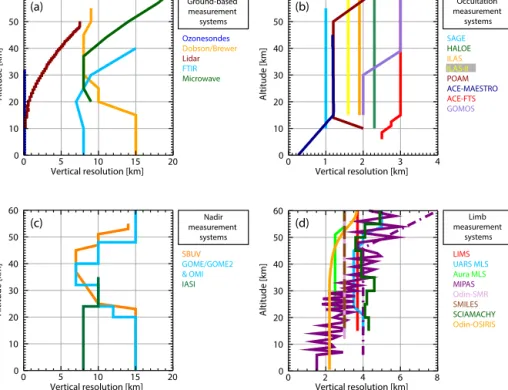
0 5 10 15 20 Vertical resolution [km] 0 10 20 30 40 50 60 Altitude [km] Ground-based measurement systems Ozonesondes Dobson/Brewer Lidar FTIR Microwave
(a) measurement Occultation
systems Vertical resolution [km] Altitude [km] SAGE HALOE ILAS ILAS-II POAM ACE-MAESTRO ACE-FTS GOMOS 0 1 2 3 4 0 10 20 30 40 50 60 (b) Vertical resolution [km] Altitude [km] Nadir measurement systems SBUV GOME/GOME2 & OMI IASI 0 5 10 15 20 0 10 20 30 40 50 60 (c) Vertical resolution [km] Altitude [km] Limb measurement systems LIMS UARS MLS Aura MLS MIPAS Odin-SMR SMILES SCIAMACHY Odin-OSIRIS 0 2 4 6 8 0 10 20 30 40 50 60 (d)
Figure 3. Vertical resolution shown as function of altitude for each of the described instruments systems: (a) ground-based instruments, (b) solar/stellar occultation instruments, (c) nadir-measuring instruments, and (d) limb-measuring instruments. The SMILES profile in panel (d) is shown as a brown dashed line that is plotted on top of the ODIN-SMR (light purple). Note that there are two profiles shown for
MIPAS in panel (d): the solid purple line represents the KIT retrieval, and the dash-dotted purple line represents the Bologna retrieval. The oscillating altitude resolution of the MIPAS KIT profile is a consequence of the evaluation of the averaging kernels on a vertical grid finer than the tangent altitude spacing: the vertical resolution is best at the tangent altitudes and coarsest between the tangent altitudes. Retrieval resolution for the Oxford and ESA processors is comparable to the KIT results; however, a courser grid is used for the retrieval and thus it does not show the oscillating features of the KIT processor. For more detail on the different MIPAS retrievals see Sect. 3.3.4.
However, measurement stability can be affected by instru-mental artifacts such as alignment error, changes in the inten-sity of the lidar signals due to varying laser power, or changes in weather conditions (Godin-Beekmann et al., 2003).
There are twelve stratospheric ozone lidar instruments op-erational globally at this point (see Fig. 1), with the longest continuous records starting in the late 1980s (Steinbrecht et al., 2009). Data are archived in the NDACC database (see Table 1d for the URL).
2.4 FTIR
Ground-based FTIR (Fourier transform infrared spec-troscopy) solar absorption measurements are performed over the 600–4500 cm−1 spectral range, under clear-sky
condi-tions using primarily high-resolution spectrometers such as the Bruker 120M (or 125M) or Bruker 120HR (or 125HR). The spectrometers can achieve a spectral resolution of 0.0035 and 0.002 cm−1, respectively. The advantage of the FTIR technique is that, for atmospheric gases such as ozone which have very narrow lines, an absolute calibration is not needed; the ozone absorption signatures are self-calibrated with the reference being the surrounding continuum. Nevertheless,
for the determination of absorber profiles and of vertical trends, especially in the upper-stratosphere, it is important to regularly monitor the instrumental line-shape. This is achieved with gas cell measurements (Hase et al., 1999).
In addition to total columns, low-vertical-resolution pro-files can be obtained from the temperature and pressure de-pendence of the absorption line shapes. Two profile retrieval algorithms are widely used, PROFITT9 (Hase, 2000) and SFIT2 (Pougatchev et al., 1995); both are based on the op-timal estimation method (Rodgers, 2000). A European FTIR network has been optimized by using a common retrieval strategy to derive ozone trends (1995–2005) in 4 layers (Vigouroux et al., 2008), one in the troposphere and three in the stratosphere, up to about 45 km (Table 1a, b). Thus, a high degree of freedom for the signal (DOFS ≈ 4.5) is achieved with the use of the 1000–1005 cm−1window (Bar-ret et al., 2002). The random error on total columns is about 2–4 % (García et al., 2012; Vigouroux et al., 2008); the lead-ing error source belead-ing the temperature. The estimated ran-dom error on the ozone partial columns can vary a little de-pending on the station (different instrument, ozone natural variability impacting the smoothing error). For example, at
Kiruna the random error for the layers ground-10 km, 10– 18 km, 18–27 km, and 27–42 km are 10, 7, 9, and 6 %, re-spectively (Vigouroux et al., 2008). The smoothing error is dominant in the two lowest layers, whereas the temperature error dominates in the middle and upper stratosphere. Further improvement (on-going research, not applied to the NDACC network yet) can be achieved by retrieving a simultaneous temperature profile, thus reducing the total column random error to less than 1 %, and the upper stratospheric error to 3 % (García et al., 2012). The systematic error is dominated by the uncertainties of the spectroscopic parameters (line in-tensity and air broadening coefficient). The systematic error due to the line intensity uncertainty was estimated to 2–3 % (Barret et al., 2003; Schneider et al., 2008) on total and par-tial columns. The error due to the air broadening coefficient uncertainty is negligible for total columns but can be as large as 4 % when partial columns are concerned (Barret et al., 2003; Schneider et al., 2008). Other sources of systematic errors, such as the temperature or the instrumental line-shape (if not correctly determined), should also be considered in the upper layers (García et al., 2012).
The ozone trends in Vigouroux et al. (2008) were calcu-lated with a bootstrap re-sampling method, applied to the daily mean partial columns of the ozone time series. This work was extended up to 2009 in the WMO 2010 ozone assessment report (WMO, 2011) for five European stations (28◦N to 79◦N). A current update up to 2012 is ongoing, in-volving additional stations, including stations in the Southern Hemisphere. The spectroscopic database has been changed to HITRAN 2008 (Rothman et al., 2009), and an additional effort of homogenization has been made in contrast to the work described in Vigouroux et al. (2008); all stations are using a priori information from the model WACCM.
The length of the FTIR ozone time series varies by tion (see Fig. 1 for the geographical distribution of the sta-tions); the longest time series available starts in 1995, and the shortest in 2002 (Fig. 2; Table 1c). In the coming years, more recently established observatory stations (e. g. Reunion Island: measurements started in 2009; Toronto: regular data containing the 1000–1005 cm−1range started in 2010) or sta-tions that have not yet reprocessed their retrievals using the optimized common strategy (e.g.: Eureka, Bremen) could be included in ozone trends studies.
The FTIR data not yet available on the NDACC database (see Table 1d for the URL) can be acquired by direct con-tact with the responsible principal investigator. There are cur-rently 17 active long-term NDACC FTIR sites. An additional long-term site (Kitt Peak, AZ, USA (31.9◦N, 111.6◦W)) has data from 1978–2005, but operations have unfortunately ceased.
2.5 Microwave
The NDACC microwave ozone profiling instruments mea-sure the spectra of emission lines produced by thermally
excited, purely rotational ozone transitions at millimeter wavelengths. All are based on the same principles but dif-fer in technical details. All use a sensitive heterodyne down-converter (receiver) that produces a replica of the spectrum it receives from the sky at a much lower so-called interme-diate frequency where it can be processed by a filter bank or digital FFT spectrometer. In all systems, the spectral in-tensity scale is established by substituting the thermal radia-tion from two black body sources for the radiaradia-tion from the sky at the receiver input. One source is at ambient tempera-ture, the second is typically chilled using liquid nitrogen. The ozone altitude distribution is retrieved from the details of the pressure broadened line shape, typically using various im-plementations of the optimal estimation method of Rodgers (1976). The attenuation of the ozone signal in the tropo-sphere is determined by measuring the tropospheric thermal emission and relating the tropospheric opacity to its emis-sion using a radiative transfer model. Stratospheric aerosols do not affect microwave measurements because the wave-length is large compared to the aerosol particle size. The altitude range is between about 20 and 55–72 km, depend-ing on the instrument (Table 1a, b). The fundamental na-tive measurement units are mixing ratio vs. pressure. The instruments operate continuously, and profile retrievals are obtained in weather ranging from clear to some overcast con-ditions. Temporal resolution can be hourly or less, so diurnal variations of ozone in the stratosphere and mesosphere can be observed.
The instruments at Lauder (New Zealand), Bern and Pay-erne (Switzerland), and Mauna Loa/Hawaii (USA) have operated essentially continuously from 1992, 1994, 2000, and 1995 to the present respectively. Ny Ålesund (Nor-way) has been making measurements since 1994, with some extended breaks. These are NDACC Primary Instruments listed in http://www.iapmw.unibe.ch/research/collaboration/ ndsc-microwave/instruments/index_spe.html. Other instru-ments, also listed on the above site, have operated over periods of months to a decade (Table 1c). Instru-ment and measureInstru-ment details for Lauder and Mauna Loa were published in Parrish et al. (1992), for Pay-erne in Maillard-Barras et al. (2009) and Hocke et al. (2007), for Bern in Studer et al. (2013), for Ny Ålesund in Palm et al. (2010). Data from these instruments are archived on the NDACC webpage (see Table 1d for URL).
Theoretical investigations of microwave ozone measure-ment errors and vertical resolution have been reported by Connor et al. (1995) and Palm et al. (2010). The former is applicable to the Lauder and Mauna Loa measurements, the latter to the Ny Ålesund measurements. As the ver-tical resolution of microwave measurements can vary by amounts approaching a factor of two from one instrument to another, it is important to download the averaging kernels along with the data and consider them in the analysis when comparing microwave measurement results. Discussions of the averaging kernels and vertical resolution are found in
Connor et al. (1995) and Caliesi (2000). The values shown in Fig. 3a are an ensemble average. Because instrument cal-ibration is based on temperature it can theoretically be kept stable over long periods of time. In practice, a more impor-tant issue is that the details of the spectral line shape must be measured with a precision that is technically challenging to achieve. The types of spectral errors most commonly en-countered tend to propagate into profile errors in the lower to middle stratosphere. Despite these challenges, the pro-files of the Mauna Loa and Lauder instruments were found to agree with others to within < 5 % from ≈ 22 to 65 km during formal blind intercomparison campaigns involving several types of instruments (McDermid et al., 1998a, b; McPeters et al., 1999). Differences between the Bern (Studer et al., 2013) instrument and others mostly fall within ≈ 7 %, as do those at Payerne up to ≈ 50 km. Relative drifts be-tween the Lauder and MLO measurements and those made with lidar, ozonesonde, SAGE II, and HALOE were typi-cally < 0.5 % yr−1 from 22 to 60 km over the period from the mid-1990s to the mid-2000s (Boyd et al., 2007). While no decadal-scale drift tests have been reported for the other stations, Steinbrecht et al. (2009) found that the Bern mea-surements were very consistent with others over the period from 1994 to 2008.
3 Satellite-based measurement systems
In the following paragraphs several satellite-based systems measuring ozone profiles are described. Systems are grouped according to measurement technique. The solar occultation technique provides spectral measurements with a very high signal-to-noise ratio allowing the detection of species with low concentrations without the need for averaging measure-ments. This self-calibrating method is less susceptible to changes in instrument performance over the mission life-time because of the reference exo-atmospheric measure-ments used in the retrieval. Stellar occultation measuremeasure-ments are relative by definition and therefore they are less sensitive to instrumental degradation. Due to the multitude of stars, global coverage is obtained. Since stars are point sources, the pointing information is excellent (uncertainty < 30 m) and the vertical resolution very good, about 2 km around the ozone maximum and below. The limb viewing technique of-fers high sensitivity to a number of trace gases with vertical resolution between 1 and 3 km (depending on instrument and wavelength) and provides day and night retrievals (only day retrievals for limb-scatter instruments), with dense sampling along the sub-orbital tracks and hundreds to a few thousands of profiles per day. Self-calibration is typically provided by reference views to (stable) cold space and onboard blackbody targets, whereas limb-scatter instruments either use the ex-traterrestrial solar spectra or limb measurements at upper tan-gent height(s) for normalization. Nadir viewing instruments provide full global coverage of the Earth on a daily basis,
with 6 km vertical resolution for the stratospheric ozone pro-file, and between tens and hundreds of thousands of profiles per day. Detailed information on ozone data collected by limb sounders, their vertical and spatial resolution, and com-parisons between individual ozone climatologies for long-term changes is provided in a study by Tegtmeier et al. (2013) about the Stratospheric Processes and their Role in Climate (SPARC) initiative on trace gas and aerosol climatologies.
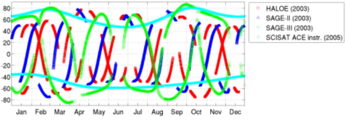
Temporal coverage of each measurement system is shown in Fig. 2. Average spatial coverage for the solar-occultation instruments is shown in Fig. 4 since this is very distinct for each of the systems. Spatial coverage for the stellar-occultation, limb and nadir systems described in the follow-ing sections is shown in detail in Toohey et al. (2013), and is therefore not explicitly repeated here. Figure 3b–d show in detail the vertical resolution of each of the satellite measure-ment systems that are described below.
3.1 Solar-occultation instruments
3.1.1 SAGE
All of the Stratospheric Aerosol and Gas Experiment (SAGE) instruments (SAGE I on the Applications Explorer Mission-B (AEM-B), SAGE II on the Earth Radiation Bud-get Satellite (ERBS) and SAGE III on the Meteor-3M space-craft), used solar occultation to take spectral transmission measurements along a slant path through the atmosphere. SAGE III added lunar occultation measurements. The SAGE instruments scanned a small field of view across the solar disk every 2 s. The wavelength-dependent atmospheric trans-mission is determined by taking the ratio of a measurement looking through the atmosphere to one taken when the sun or moon is above the atmosphere as seen from the spacecraft. The systematic uncertainty of the transmission is indepen-dent of instrument characteristics as long as the instrument is stable over the brief few minutes spanned by each occultation event. Ozone is inferred from spectral measurements near 600 nm, at the peak of the Chappuis band and nearby chan-nels are used primarily to characterize the spectral aerosol extinction. The small field of view and high signal-to-noise ratio enabled by looking at such bright sources enables the retrieval of the ozone profile at 1 km vertical resolution with low random uncertainty (≈ 1 %) from just below the tropopause to well above the stratopause (Table 1a, b).
SAGE I made measurements over a 33 month period, start-ing in February 1979 (Fig. 2). SAGE II made measurements for 21 years starting in October 1984 (Table 1c) covering the time when ozone depletion was at its peak as well as dur-ing the transition to lower chlorine loaddur-ing in response to the Montreal Protocol. SAGE III made measurements from December 2001 to December 2005; it provided complemen-tary high-latitude coverage (Fig. 4).
The solar occultation technique produces a very stable long-term data set. The ratio between scans across the solar
Figure 4. Latitudinal coverage for the solar-occultation instruments
(example years: 2003 and 2005). SAGE I is similar to SAGE II (blue triangles), POAM and ILAS instruments are similar to SAGE III (turquoise triangles).
disk above the atmosphere and scans through the atmosphere to determine the spectral extinction vs. altitude are calcu-lated. The instrumental radiometric properties divide out in this ratio. Scanning across, rather than staring at, the sun pro-vides accurate knowledge of the altitude registration of each measurement.
The most recent version of the SAGE data is version 7. This is the first version that will unify the algorithm, an-cillary data and spectroscopy across all three SAGE mis-sions (Damadeo et al., 2013). Data are archived at the Atmo-spheric Science Data Center, NASA Langley Research Cen-ter in Hampton, Virginia (see Table 1d for URL).
3.1.2 HALOE
The Halogen Occultation Experiment (HALOE) was launched aboard the Upper Atmosphere Research Satellite (UARS) in 1991 and operated successfully for fourteen years until November 2005. HALOE made global observations verifying the effects of chlorine compounds on the chemical loss of ozone in the upper stratosphere. In addition to HCl and ozone, HALOE provided profile measurements of H2O,
CH4, NO, NO2, HF, temperature and aerosol extinction
us-ing the technique of solar occultation. Its measurements of HF, HCl, CH4, and NO were obtained using gas filter
corre-lation radiometry. HALOE ozone transmission profiles were measured by the more traditional method of broadband filter radiometry (Russell III et al., 1993), using a broadband chan-nel from 9.2 to 10.4 micrometers. Overall measurement un-certainties range from 9–25 % in the lower stratosphere and from 9–20 % in the upper stratosphere and mesosphere.
The HALOE retrieval algorithm employed a top-down, onion-peeling approach and iterated the calculated tangent-layer transmissions to achieve a match with the measured transmissions from each of its channels. Measured transmis-sions are calibrated according to their solar look values at top of scan. The one exception was the method for obtaining the temperature profile, which began with the assignment of the co-located National Center for Environmental Prediction (NCEP) temperature and pressure (or T (p) value) at 31.5 km to the HALOE-measured CO2 channel transmission profile
at that same level. Then, a first-guess T (p) profile was iter-ated and proceeded upward by matching the calculiter-ated trans-mission value in each tangent layer with that observed in the HALOE CO2channel centered at 2.8 µm. The measured
transmission profiles for all the species, including ozone, were then registered vs. the pressure profiles obtained in this way, prior to final retrievals of the species volume mixing ra-tio profiles (Table 1a–c). The HALOE Level 2 profiles can be downloaded from the NASA Goddard Earth Sciences Data & Information Services Center (GES DISC) or the HALOE webpage (see Table 1d for the URLs).
3.1.3 ILAS and ILAS-II
The Improved Limb Atmospheric Spectrometer (ILAS) was a satellite-borne solar-occultation sensor on board the Japanese Advanced Earth Observing Satellite (ADEOS) (Sasano, 2002). ILAS consisted of an infrared spectrometer that covers the wavelength region from about 6 to 12 µm with a detector array of 44 elements and a visible spectrometer from 753 to 784 µm with a detector array of 1024 elements. ADEOS was successfully launched in a sun-synchronous or-bit on 17 August 1996. After a 3 month initial checkout pe-riod, continuous operation of ILAS started on 30 October, lasting until 29 June 1997 when a failure in the satellite’s so-lar battery system occurred (Fig. 2). For a period of about 8 months, ILAS made solar-occultation measurements at 57– 71◦N and 64–88◦S, and collecting ≈ 6700 profiles of O3,
HNO3, NO2, N2O, CH4, H2O and aerosol extinction
coeffi-cients at 780 nm.
ILAS-II was a satellite-borne solar-occultation sensor on board the satellite ADEOS-II (Nakajima, 2006). ILAS-II consisted of four spectrometers: an infrared spectrometer (between 6.21 µm to 11.76 µm); a mid-infrared spectrome-ter (between 3.0 µm and 5.7 µm); a high-resolution infrared spectrometer (between 12.78 µm and 12.85 µm); and a visible spectrometer (between 753 nm and 784 nm). ADEOS-II was successfully launched on 14 December 2002, also in a sun-synchronous orbit. After a 3 month initial checkout period, continuous operation of ILAS-II started on 2 April 2003, lasting until 24 October 2003 when the satellite’s solar bat-tery system malfunctioned (Fig. 2, Table 1c). For a period of about 7 months, ILAS-II made solar-occultation mea-surements at 57–71◦N and 64–88◦S, and gathered ≈ 5700 profiles of O3, HNO3, NO2, N2O, CH4, H2O, ClONO2,
N2O5, CFC-11, CFC-12 and aerosol extinction coefficients
at 780 nm.
Ozone and other minor gas vertical profiles were retrieved by applying both the onion-peeling method and the nonlin-ear least-squares fitting method. Version 5.20 ILAS and ver-sion 1.4 ILAS-II ozone profiles were validated by comparing with various data sources (Sugita et al., 2002, 2006). These validations showed that ILAS ozone data agreed with other data sets within ±10 % with a few exceptions between 11 and 64 km (Table 1a, b). ILAS-II ozone data agreed with