Determination of Drivers of Stock-Out Performance of Retail
Stores using Data Mining Techniques
by
Khalid Usman M.B.A International Aviation
Concordia University. 1999. B. Eng Avionics Engineering PAF Academy, Pakistan. 1994.
Submitted to the Engineering Systems Division in Partial Fulfillment of the Requirements for the Degree of
Master of Engineering in Logistics
at the
Massachusetts Institute of Technology
June 2008 © 2008 Khalid Usman. All Rights Reserved
The author hereby grants to MIT permission to reproduce and to distribute publicly paper and electronic copies of this thesis document in whole or in part.
Signature of Author ... ... ....
Master of Engineeri j L~ ics Pn ginp g Systems Division
7 /May 9, 2008 Certified by... Accepted by ... MASSACHUM S N ' EN OF TEO•NOLOQG Y
AUG
0 6 2008
LIBRARIES
• ~.'..•...o... - v / i Dr. Chris CapliceExecutive Director, Master of Engineering in #gistics Program
Executive Director, Center for Trispo ion and Logistics Thesis Supervisor
V /// . Prof. Yossi Sheffi Professor, Erg neering Systems Division Professor, Civil and Environmental Engineering Department Director, Center for Transportation and Logistics Director, Engineering Systems Division
Determination of Drivers of Stock-Out Performance of Retail
Stores using Data Mining Techniques
by
Khalid Usman
Submitted to the Engineering Systems Division on May 9, 2008 in partial fulfillment of the
requirements for the degree of Master of Engineering in Logistics
Abstract
This research applies data mining techniques to give a picture of the interaction of
performance variables such as between stock-outs and store attributes, and stock-outs and other variables including store sales, income and demographic data, as well as various aspects of inventory management data. This research uses three data mining techniques: multiple ordinary-least-squares (OLS) regression, logistic regression and data clustering. The first part of the research evaluates how the effect of stock-outs at the distribution center (DC) level impacts the downstream sales at the store-level. Using multiple
regression techniques, it was observed that stock-outs at the distribution center level have a detrimental impact on the sales at the retail store level.
The second part of the project focuses on understanding the relationships of store stock-out performance to various drivers. The variables that were determined to be drivers of store performance include income level of the area, demographic profile, years the store has been in operation, day of the week delivery from distribution center, distance of store from the distribution center and average inventory-on-hand. Using data clustering
techniques, worse performing and good performing clusters of stores were identified. The two worse performing clusters were 'Low-Income, Newer' stores and 'Newer, Further
from DC' stores. The three good performing clusters were 'High-Income, High-Inventory'
stores, 'Closer to DC, Older' Stores and 'High-Income, Smaller' stores.
Thesis Supervisor: Dr. Chris Caplice
Title: Executive Director, Masters of Engineering in Logistics Program Executive Director, Center for Transportation and Logistics
Acknowledgements
I am extremely thankful to a number of people who have been extremely helpful in
providing their help and support during this thesis. Firstly, I would like to thank my thesis advisor, Dr. Chris Caplice. Despite his busy schedule, Chris has always been able meet with me on a regular basis, guide me on the research and provide me thorough feedbacks on my thesis draft.
I would also like to thank Marinko Kondic from Unilever who has been available
on a very regular basis for discussion on all the facets of the business and help me understand them. I would also like to thank Aviv Langus who provided all the data from Unilever and often on very short notice. The research would not have been successful without the very active support of Unilever and these individuals.
Another person that I would like to extend my sincere thanks is instructor of my technical writing class, Dr. Bill Haas. Bill was always available inside and out-of-class to review my thesis and provide very valuable feedback which helped improve my writing.
Finally, I would like to thank my parents and my family for being a constant source of motivation to pursue the rigorous academic life of MIT and stay on course throughout my research and thesis.
Khalid Usman Cambridge, MA
Table of Contents
Abstract 2 Acknowledgements 3 Table of Contents 4 List of Tables 5 List of Figures 6 1 Introduction 7 2 Literature Review 92.1 Data Mining and its application 9
2.2 Stock-outs and their Impact 10
2.3 Root causes of Stock-outs 13
3 Methodology 17
3.1 Data gathering 17
3.2 Measurement of Stock-outs 18
3.3 Multiple Regression 20
3.4 Logistic Regression Analysis 23
3.5 Cluster Analysis 25
4 Impact of Stock-outs at the Distribution Center 28
4.1 Regression modeling to determine Impact of Stock-outs at the
Distribution Center 28
5 Data Mining to Determine Drivers of Stock-out 33
5.1 Drivers of Stock-out - Using Multiple Regression 33 5.2 Drivers of Stock-out - Using Logistic Regression 39
5.3 Data Clustering Approach 45
6 Recommendations and Future Research 59
6.1 Managerial Insights 59
6.2 Recommendations 62
6.3 Future Research 64
Bibliography 66
List of Tables
Table 1: Differences between hierarchical and non-hierarchical methods of
data clustering 26
Table 2: Regression model on aggregate basis 29
Table 3: Regression model for category 'Beauty-Care' 30
Table 4: Regression model for category 'Home Cleaning' 30 Table 5: Regression model for category 'Candy and Snacks' 31
Table 6: Regression model for category 'Food' 31
Table 7: Regression model giving the drivers of stock-out 35 Table 8: Logistic Regression model giving the drivers of stock-out 40 Table 9: Odds ratio estimates for logistic regression model 42
Table 10: Data clustering summary for 10-clusters 47
Table 11: Stock-out performance of good and worst performance clusters relative
to the average for all stores 48
Table 12: Comparison of attributes of worst performing clusters vs. overall store
population 50
Table 13: Similarities and differences between Cluster-9 and Cluster-10 based on
the t-statistic test 53
Table 14: Comparison of attributes of good performance clusters vs. overall store
population 55
Table 15: Similarities and differences between Cluster-5, Cluster-4 and Cluster-8
List of Figures
Figure 1: Consumer response to out of stock situation 11
Figure 2: Percentage of Out of stock for different regions across the world 13
Figure 3: Graph showing causes of out of stock 15
Figure 4: Sales at an SKU/store level which are used to measure stock-outs 20
Figure 5: Distribution of stock-outs for all stores 21
Figure 6: Stock-out instances by week for 8 high-moving SKUs 24 Figure 7: Demand variability for stores by number of years the stores have been 39
in operation
Figure 8: Impact of backroom size on stock-out levels 44
1
Introduction
RetailerCoI is currently a VMI (vendor managed inventory) account with Unilever Home & Personal Care (HPC) business. Unilever has 150 active SKUs that are carried in 8200 RetailerCo stores in the United States. RetailerCo operates 9 distribution centers (DCs) in the United States and Unilever has 5 distribution centers in the US. The replenishment of items is from Unilever DC to RetailerCo DC, and then to the individual RetailerCo
General Stores. At times, due to supply chain issues, a particular SKU will be out-of-stock at a RetailerCo store which causes lost revenue potential for both RetailerCo and Unilever. According to Unilever, the out-of-stock rate for the retail industry stands around 6-10% and its stock-out percentages are in line with the industry rate.
This research project uses data mining techniques to explore the data that is available through the VMI partner. The data available from the VMI partner is point of sale, inventory management, and store profile data. Demographic data, such as income levels in areas and population characteristics, which is available from the census bureau is also used. By using data mining techniques, we will distinguish performance variability from store to store and determine the drivers of stock-out that are causing it. RetailerCo stores comprise around $200 million of business annually for Unilever, and Unilever expects that a 2-3% improvement in in-stock performance will generate a benefit of more than $1 million.
Section 2, "Literature Review" surveys previous works on the drivers and impact of stock-outs. Section 3, "Methodology" explains the three different data mining techniques that have been utilized. It also gives the data sources used for the research and the method
developed to measure stock-out for the purpose of my research. Section 4, "Impact of Stock-outs at the Distribution Center" deals with the data analysis to determine the impact of stock-out at the distribution center level and the modeling results. Section 5, "Data Mining to Determine Drivers of Stock-out" gives the data mining techniques used to determine the drivers of stock-outs. In this section, the results of the models that have been developed are given and the results have been discussed. Finally, section 6,
"Recommendation and Future Research", goes on to provide the managerial insights, recommendations and the future research opportunities that exist in the area of data mining and stock-out performance.
2
Literature Review
Data mining has not been fully utilized in supply chain management and specifically for determining the drivers of stock-out in retail performance. In this section I will discuss the research and studies that comprise the body of literature concerning retail stock-outs, its drivers and impacts.
2.1
Data Mining and its Applications
Data mining involves finding patterns in large datasets, and it does so in an open-ended fashion, without putting strict limits on the business question being addressed (that inference would require). Classical statistics places emphasis on inference (determining whether or not a pattern or interesting result might have happened by chance). Data
mining, on the other hand, is a clean slate approach to determine relationships and impacts among different business variables (Shmueli, 2007). Data mining has evolved with the growth of the data itself. With large corporations keeping and storing huge amount of data, there is an immense potential to utilize all the data and use sophisticated data mining techniques which have not been used before due to constraints on storage or computing power. Many of the exploratory and analytical techniques used in data mining would not be possible without today's computational power.
There are several techniques of data mining: Regression modeling, logistic
regression, discriminant analysis, neural networks and cluster analysis are some of the data mining techniques which are used in different areas of decision sciences. While some of these techniques are better for developing predictive models, some of them are more
effective in developing exploratory models where the impact of different business drivers can be ascertained on the outcome. Ordinary-least-squares (OLS) Regression and logistic regression are both good candidates for building predictive models as well as models which can explain the inter-relationships of business drivers. Data clustering is a technique to form groups or clusters of similar records based on several measurements made on these records (Shmueli, 2007).
2.2
Stock-outs and their Impact
Discussions of inventory usually revolve around the classical sawtooth inventory model which has been summarized by Tersine (1998). This model describes how inventory levels fluctuate as inventory is received and consumed. It is also used to illustrate the concepts of a stock-out, cycle stock and safety stock, backordering, and how all stock-outs are the result of some variation in product supply, demand or a combination of both.
A stock-out for a retailer is defined as an event where a retailer experiences a demand for an item that is not available in inventory. Stock-out situations are detrimental for both manufacturers and the retailers. The real cost of stock-out is difficult to measure because it differs as a function of consumer response to the stock-out. According to Gruen, Corsten and Bharadwaj (2002), in case of a stock-out, the consumer may decide to:
* Substitute the item,
* Delay the purchase of the item,
* Leave the store and either forgo the purchase or search for the item somewhere else, or
* Do not purchase the item again (lost sales).
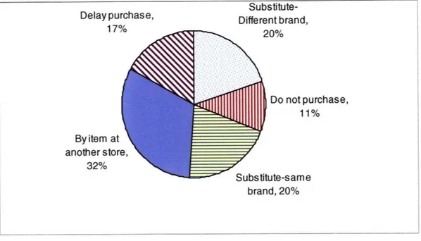
A stock-out situation leads to a consumer response which results in either loss of sale to a manufacturer or a retailer or both. Studies on the consumer response to stock-out situations show an increasing willingness of consumers to seek the out-of-stock items at an alternative outlet. Figure 1 gives the breakdown of the consumer response to the out-of-stock situation.
Substitute-Delay purchase, Different brand,
17% 20% Do not purchase, 11% ute-same brand, 20%
Figure 1: Consumer response to out-of-stock situation (Source: Retail Out-of-Stocks: A Worldwide Examination of Causes, Rates, and Consumer Responses.)
A study conducted by the Grocery Manufacturer's of North America determined that in case of stock-outs retailers lose the sale 41% of the time while suppliers lose sale 28% of the time. So, there are uneven impacts of stock-outs which can influence how much it costs to each party in terms of stock-outs.
By item at another stor
Retailing is becoming increasingly competitive and with decreasing margins. Therefore, it is of paramount importance for retailers and manufacturers to ensure that the right product is available at the right time at the right place. At the same time, the number of products in the stores is increasing which makes the management of inventory more complex. According to Food Marketing Institute (FMI) statistics, the number of SKUs in 2001 in an average grocery store was nearly 25,000. This makes the task of keeping products in stock and available very difficult and something that has to be coordinated among different channels. Stores implementing management systems such as Efficient Consumer Response2 (ECR) and Quick response3 (QR) have shown less instances of stock-outs (Gruen, Corsten and Bharadwaj, 2002). Also, bigger stores, like Wal-Mart, by virtue of their power over suppliers are able to offer better service levels. Therefore, managing stock-out levels will increasingly become a source of strategic advantage because product availability by competing retailers will be lesser. According to Gruen, Corsten and Bharadwaj (2002) research has indicated that by lowering stock-outs, retailers can increase earnings by up to 5 percent.
The fist stock-out study conducted nearly 40 years ago reported stock-out rates at 12.3 percent (Progressive Grocer 1968). Recent studies, however, report a stock-out rate between 7 to 10 percent (Anderson Consulting 1996, Gruen, et al. 2002, Roland Berger 2003). Statistics compiled by Grocery Manufacturers of America (GMA) on 661 stores in
2 Efficient Consumer Response (ECR) is characterized by the emergence of new principles of collaborative
management along the supply chain by which companies can serve consumers better, faster and at a less cost by working together with trading partners.
Quick Response (QR) also known as rapid response was developed in the 1980s. The basic idea of QR is to
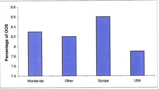
29 countries, point at the worldwide average of stock-out levels are around 8.3%, although this percentage varies geographically as shown in the Figure 2.
Figure 2: Percentage of Out-of-stock (OOS) for different regions across the world (Source: Retail Out-of-Stocks: A Worldwide Examination of Causes, Rates, and Consumer
Responses.)
If a store is consistently out-of-stock, it may have a detrimental affect on the
customer base; either by consumers who experience stock-out or by word-of-mouth and negative publicity from other who have frequently experienced it.
2.3
Root causes of Stock-outs
Stock-outs can be caused due to business practices or inefficiencies in store operations, distribution center, retailer headquarter or supplier. According to Corsten and Gruen
(2003) causes of stock-outs include: * Product purchasing frequencies,
* Large number of SKUs,
* Bad Point-of-sale data and data inaccuracies, * Forecasting issues and ordering problems, * Insufficient staffing or busy staff,
* Backroom issues, and congested backrooms, * Receiving errors and inaccurate records,
* Shelf replenishment infrequency and late or no shelving, * Shrinkage of the product caused by damage or theft,
* Ordering practices of distribution center (no order, late order or wrong backorders), * Promotion and pricing decisions at retailer headquarters,
* Transportation, receiving and storage practices at distribution centers, and * Longer lead time issues for replenishment from DC.
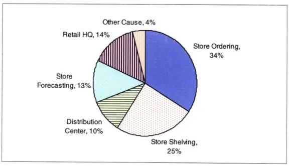
The table for root-causes of stock-outs at the level of store, DC, retailer headquarter and supplier is given in Appendix A. Figure 3 shows the reasons for out-of-stocks into the major categories, the biggest one being store ordering.
Other Cause, 4%
Figure 3: Figure showing causes of out-of-stock (Source: Retail Out-of-Stocks: A Worldwide Examination of Causes, Rates, and Consumer Responses.)
'Store Ordering' issues (34 percent) mean that the retailer may have ordered too little or too late so that the distribution center could not deliver before the retail store ran out of the item. 'Store Forecasting' issues (13 percent) mean that the retailer may have forecasted the demand for an SKU below the actual demand and ordered an insufficient supply. Often promotional items are forecasted with great inaccuracies and can cause items to run out on shelf. 'Store Shelving' issues (25 percent) are mostly due to replenishment practices within the store. The product could be in the store in the backroom, or some other area of the store but it not available on the shelf once the customer wants it. 'Distribution Center' issues (10 percent) are the replenishment issues that occur upstream of the retail store. The distribution center may have insufficient inventory to meet the demand of the store and causes delays in getting the required items to the stores. 'Retail HQ' issues (14 percent) are caused due to planning and management problems which can include
Retail HQ ore Ordering, 34% Store Forecasting, 13% Distribul Center, 1 Store Shelving, 25%
inadequate shelf-space allocation and lack of communication between the retailer warehouse and headquarters.
Based on the statistics given above in the figure, about 70 to 75 percent of stock-outs are a direct result of retail store practices, which include forecasting, ordering and
store shelving. Also, almost half (47 percent) of stock-outs occur from store ordering and forecasting processes. According to Angerer (2005), inaccurate point-of-sale and inventory data in automatic shelf replenishment (ASR) systems can generate inaccurate forecasts and orders as well.
3
Methodology
My research uses three data mining techniques to determine the drivers of stock-out and to
differentiate retail stores by level of performance. This section describes the three data mining techniques: Multiple regression, Logistic regression, and Data clustering. After section on data gathering and measurement of stock-outs, each sub-section below explains the suitability of the techniques used to the stock-out issue being considered.
3.1
Data gathering
The pre-requisite for data mining is to get all the relevant data from the available sources and setup the data accordingly for data analysis to be performed. The primary source of data in my research was point-of-sale (POS data) as well as data from the inventory system of RetailerCo. I utilized the following four sources of data for my research: Point-of-Sale and inventory data available through Verisign/Retailsolutions, Store characteristics data provided by Unilever, Latitude/Longitude information to calculate mileages, and US Census bureau decennial census data (2000) to derive demographic variables such as population characteristics, income etc.
I selected 8 high-moving SKUs to conduct the analysis and point-of-sale data was extracted for these high velocity items for one full year. The data is at a high level of granularity and it comprised of more than 6 million data points. To process data of this size, the statistical package of SAS was utilized.
Store characteristics data like square-footage, the number of years the stores are in operation, the DC serving the store, the zip-code in which the store is located and the day
of the week that the store gets replenishment from the distribution center was obtained from Unilever.
In addition to the store characteristics data, I obtained the geographical latitude and longitude data for the zip-codes and used the great circle mileage calculation to determine the distance between the stores and the distribution centers.
The final piece of the data was to get income and demographic characteristics of the areas in which the stores were located. US Census Bureau data was downloaded from the website and processed. Stores where certain SKUs did not have any sale for extended periods of time were filtered and a minimum threshold of sale of 1000 items for the year was used to filter out any stores with intermittent or low demand patterns. This reduced the list of stores to 4046 where the 8 SKUs were having consistent sale for the full year, as well as the overall demand was above the minimum threshold. Finally, all the sources of data were merged together to form one dataset.
3.2
Measurement of Stock-out
The biggest challenge in data collection was to obtain data on the stock-outs for the SKUs, as the retail out-of-stock is one of the most confusing metrics in the retail industry (Retail Solutions, 2008). According to Daniel and Corsten (2007), three different kinds of stock-out measurements could be used: (1) audit of physical inventory, (2) analysis of point-of-sale (POS) data and (3) user of perpetual inventory data.
In the ideal world, the data on inventory levels could indicate stock-outs. For example, when the inventory level for a particular SKU at a store is zero it would imply a stock-out
situation. However, the inventory data in the system is not an accurate reflection of what is available on the shelf, for reasons such as:
* Item is available in the backroom but is not being replenished on the shelf, * Shrinkage (stealing or damage) of the item which would cause discrepancy
between system data and actual item availability, and
* Bad retail practices, especially due to checkout counter practices which would register a sale for a similar item yet a different SKU
The correct picture of shelf-availability and hence, the stock-out data can be obtained if a store audit is conducted and that data is made available. Audit data, however, can be expensive to maintain and companies do not keep it proactively and even if the audit is done, it is for select SKUs for a short period of time.
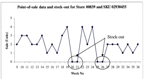
Due to the challenges in obtaining accurate and meaningful stock-out data through audits, the stock-out metric I developed was based on point-of-sale data. For the high-moving SKU items, a consistent loss of sale for a particular interval of time was used as a proxy to indicate a stock-out situation. I conducted the analysis on the sensitivity of the interval of time and discussed with supply chain staff at Unilever. This interval was
selected as a two-week time period, i.e., if the SKU has no sale for two consecutive weeks, it would comprise as one stock-out event. Figure 4, for illustrative purposes, gives the sale pattern at store 00839 and SKU 02930455 which is used to identify the conditions of stock-out. The graph clearly identifies stock-out conditions during weeks 20-21, and 25-26.
Point-of-sale data and stock-ont for Store 00839 and SKU 02930455 5 4 ~ 3
=
8 .£ 2 ~ 00 9 10 11 12 13 14 15 16 17 18 19 Week No 28 29 32 34 35 36Figure 4: Sales at an SKU/store level which are used to measure stock-outs.
3.3 Multiple
Regression
Regression analysis using ordinary-least-squares (OLS) is a technique used for modeling of numerical data and relies on the use of a dependant variable (outcome, response variable) and one or more independent variables (input variables, explanatory variables). In the case of my analysis, the dependent variable is the number of stock-outs aggregated by store for one year for which the data is collected. The data selected for this case has been limited to only 8 high-moving SKUs for one year time period. Sinceitis point-of-sale
data, the size of the data for 8 SKUs is around 3 million data points. The statistics package of SAS is utilized to handle data of this size, pre-process and summarize it and then perform regression analysis on more than 20 different attributes.
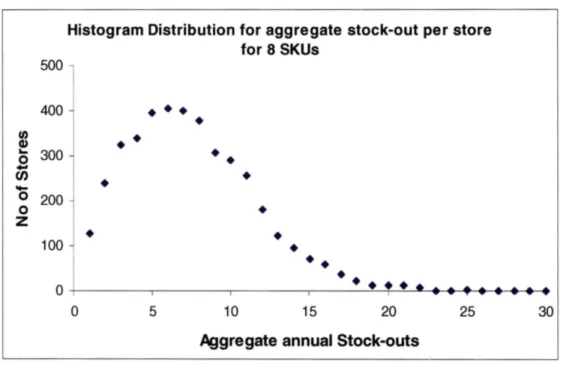
For regression analysis, each observation is the number of stock-out events for one store across the 8 SKUs and is the dependent variable. This reduces the dataset for
regression to more than 4000 observations, each comprising one store and the stock-outs for each of the store has been aggregated. The figure below gives the distribution of the stock-outs for all of the stores. The number of annual stock-outs per store is with a mean of 6.5, median of 6.0 and standard deviation of 4.1.
Histogram Distribution for aggregate stock-out per store for 8 SKUs 500 400
•••
•
tn••
CI)...
300••
0...
en•
•
....
0 200 0•
Z•
•
100•
••
••
0.
..
.
~.... ....~ ... .... ....~ ~ ....~ .... ....~ .... 0 5 10 15 20 25 30Aggregate annual Stock-outs
Figure 5: Distribution of stock-outs for all stores.
For regression analysis, the assumption is that in the population of interest the following mathematical relationship holds:
(1)
where,
/30,/31, ....
j3pare the coefficients andeis the "noise" or unexplained part and Yis the dependent variable. The data, which is a sample of the population, is then used to estimate the coefficients and variability of the noise. The approximate model can be written as:(2)
The objectives behind fitting a regression model that relates a quantitative response with the explanatory variables are, determining the relationship between the response and predictor/explanatory variables, and to predict the outcomes of new cases. The objective of my research will be to understand the relationships between the variables rather than to predict the outcomes of new cases. As an indicator of the goodness of fit, R 2 was used,
which is similar to R2 but is adjusted for the number of independent variables in the model. The closer R 2 is to 1, the more variability is explained by the model and the more likely
the model can predict the outcome.
The measure of stock-out for each store is given by:
SStockoutik , V k
i j
where, i is SKUs for which stock-out has to be measured, n is total number of SKUs, j is week number for which stock-out has to be measured, m is total number of weeks for which stock-outs have to be measured, for store k.
The formulation for the multiple regression analysis, incorporating all possible explanatory variables for which data is available, will be:
Z
Stockoutijk =f(average inventory-on-hand, day of week for store delivery, iistore demographic variables, population income variables, store layout, distance from store to the distribution center, DC serving the store, years since store has
Regression analysis will be performed on the stock-out metric for each store (response variable) and all the possible explanatory variables to determine the significant drivers impacting stock-outs.
3.4
Logistic Regression Analysis
Logistic regression analysis or logit analysis is essentially a regression model that is tailored to fit a categorical variable (in the form of 1 or 0). The independent variables in this case could be either ordinal or categorical. The regression parameters in logit analysis
are obtained using maximum likelihood method instead of ordinary-least-squares. The general form of logit model is given below, for k explanatory variables and i=l,...,j individuals:
log[ Pi I
=
a+/x +f 2Xi2 +.. +I Xik, (4)where pi is the probability that yi = 1. The expression on the left-hand side is usually
referred to as the logit or log-odds.
The model above, can be solved for pi to obtain:
1
P =
1
+exp(-a'- (5)lAxil -- 2Xi2 ...- k ik(5)
This equation has the property that no matter what values are substituted for, ''s
and the x's, pi will always be between 0 and 1.
Logistic regression analysis can be used to model the occurrence of a stock-out. The categorical variable 1 for out will be used to represent the occurrence of a stock-out at the store, SKU and week level. The event 0 will be used to represent no stock-stock-out. Hence, we can develop a logistic regression model that will predict the occurrence of
stock-outs for the 8 high volume SKUs for more than 4000 RetailerCo stores for a period spanning 50 weeks.
The stock-out response variable to be modeled is given as:
Stockoutijk ,
where, i is store out of the 4046 RetailerCo stores, j is SKU out of the 8 high moving SKUs, and k is week in the year for which the analysis will be carried out.
StockoutUk will be either 1 or 0 depending on whether that particular store had a
stock-out (1 condition) for that particular store for that SKU for that week. If there is no stock-out the value for the variable will be 0.
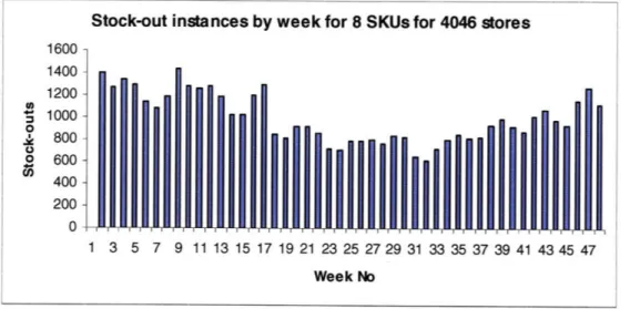
The stock-outs for the 8 high moving SKUs for the stores are given by the week of the year in the figure below. The average number of stock-outs per week was 995, with median of 935 and standard deviation of 219.
Stock-out instances by week for 8 SKUs for 4046 stores 0 061AI~J
1601400 1200 -* 1000- 800-o 600- 400-200 -0 1 3 5 7 9 11 13 15 17 19 21 23 25 27 29 31 33 35 37 39 41 43 45 47 Week No
Figure 6: Stock-out instances by week for 8 high-moving SKUs.
II
I
I I I I I I1
I I!
!
11
I11
I I -I 1 I 1 1 . . .1 T l~~ . . . .I . . .l ~ l. . lilllll IFigure 6: Stock-out instances by
week for 8 high-moving SKUs.
The independent variables will be similar to the ones used for multiple regression except that the inventory levels will be corresponding to the same level of granularity as the response variable, i.e. per store, per SKU per week.
Stockoutijk =
f
(average inventory-on-hand for SKU for the week, day of week for store delivery, store demographic variables, population income variables, store layout, distance from store to the distribution center, DC serving the store, yearssince store has been in operation) (6)
3.5
Cluster Analysis
Cluster analysis is a data mining technique that has been used to form groups or clusters of similar records based on several different attributes of these records (Shmueli, 2007). The main purpose is to form the clusters of records which are similar to each other. These clusters with similar attributes can then be analyzed for consistent patterns and to develop insights. Cluster analysis can be applied to huge amounts of data with a lot of different attributes and there are powerful software tools available with data clustering algorithms.
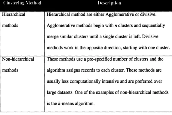
There are two general types of clustering algorithms for a dataset of n records, hierarchical methods and non-hierarchical methods (Shmueli, 2007). The difference between hierarchical and non-hierarchical methods is given in Table 1 below.
-lierarclhical methods
Non-hierarchical methods
Hierarchical method are either Agglomerative or divisive. Agglomerative methods begin with n clusters and sequentially merge similar clusters until a single cluster is left. Divisive methods work in the opposite direction, starting with one cluster. These methods use a pre-specified number of clusters and the algorithm assigns records to each cluster. These methods are usually less computationally intensive and are preferred over large datasets. One of the examples of non-hierarchical methods is the k-means algorithm.
Table 1: Table giving the difference between hierarchical and non-hierarchical methods of data clustering.
For the purpose of data clustering, k-means algorithm will be used within the research. This method starts with specifying a desired number of clusters, k, and to assign each record to one of the k clusters so as to minimize the measure of dispersion within the clusters. The goal is to divide the sample into the pre-specified number k of
non-overlapping clusters so that clusters are as homogeneous as possible with respect to the measurements used.
Forming of the clusters requires distances to be measured from each record to the cluster centroid. A common measure of within-cluster dispersion is the sum of the distances (or sum of squared Euclidean distances) of records from their cluster centroid. The whole problem of allocating records to clusters can be formulated as an optimization problem utilizing integer programming, but generally heuristic methods are used that
I
I Ir
produce good solutions. The k-means algorithm is one such method and it entails the following steps:
* User chooses k to start with the initial clusters
* At each step, each record is reassigned to the cluster with the closest centroid. * The centroids for each cluster are recomputed that gained or lost a records and the
step above is repeated.
* The algorithm is stopped when moving any more records between clusters increases cluster dispersion.
There are commercially available software that have data mining algorithms. For this research project, 'XLMiner' will be used which is an add-on to Microsoft Excel and has
4
Impact of Stock-out at the Distribution Center
In this section, regression models are developed which predict the impact on the sales at the retail stores by stock-outs at the distribution center level. Models are developed at the aggregate level as well as calibrated on the individual category of products. Finally, the results and insights obtained from the analysis are discussed.
4.1
Regression Modeling to determine Impact of Stock-out at the
Distribution center
If a store generates a demand for a stock-keeping unit (SKU) and it is not available at the distribution center to be shipped to the store in time, this creates a stock-out situation at the distribution center. This may or may not have a detrimental downstream impact at the retail store level. In this section, data analysis is carried out to determine the impact of this stock-out situation at the distribution center level. The total dollar amount of the item (Units x Price per unit) is denoted by Xout and represents the magnitude of the stock-out at the distribution center in dollar terms. If there is minimal downstream impact on store level stock-outs and eventually sales, then inventory levels at the distribution center can be kept at minimum level achieving cost savings.
I used regression analysis techniques to model the downstream impact of stock-outs at the distribution center level. For the purpose of data analysis, I used one year of sales data from the stores and also the stock-out data from distribution centers. In addition, the promotion calendar was used to identify the months for which sales promotions were
carried out. To determine the impact of downstream stock-outs we used the following mathematical formulation:
Daily Sales = a*(Daily average annual sales) + /3*(Xout) + y*(Promotion Dummy
variable * daily average annual sales) (7)
A no-intercept model was chosen because it provided a better fit for the data.
Results and Conclusion
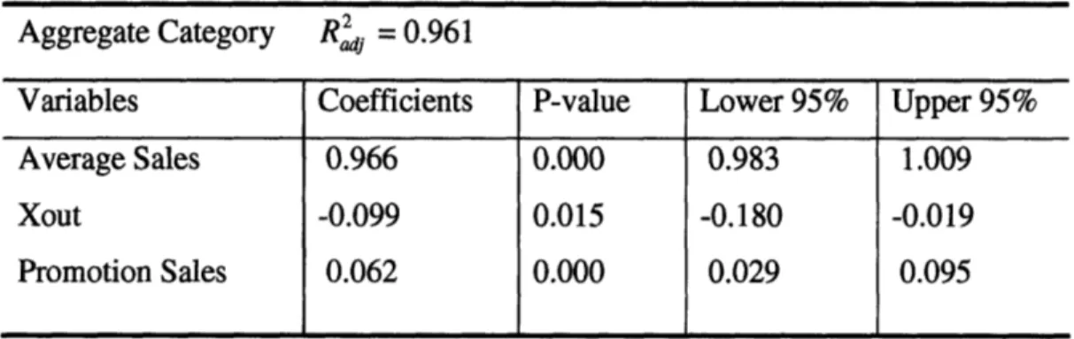
Regression models were calibrated at the aggregate level and the following individual category levels: Beauty care, Home Cleaning, Candy and snacks, and Food. Results from the individual models as well as the aggregate model were similar in portraying the impact of the Xout on the store sales. The results from the aggregate model are given in Table 2.
Aggregate Category Rp = 0.961
Variables Coefficients P-value Lower 95% Upper 95%
Average Sales 0.966 0.000 0.983 1.009
Xout -0.099 0.015 -0.180 -0.019
Promotion Sales 0.062 0.000 0.029 0.095
Table 2: Regression model on aggregate basis
The aggregate model shows that a 1 dollar stock-out at the distribution center results in a 9.9 cents loss of sales at the store level. Similarly, a promotional event boosts the sales by 6.1 percent from the average level, all other things being equal.
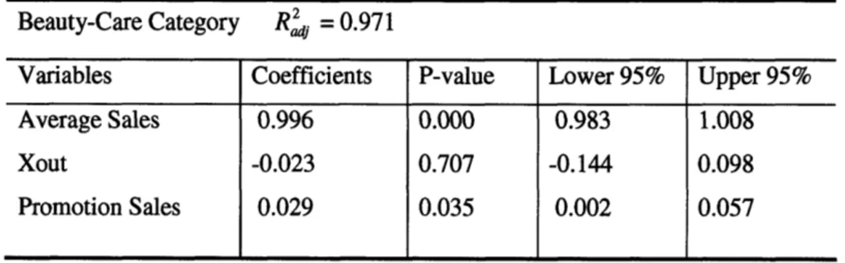
Similar regressions were performed on the individual category of items as well. The table below gives the regression results for the 'Beauty-Care' category.
Beauty-Care Category Raj = 0.971
Variables Coefficients P-value Lower 95% Upper 95%
Average Sales 0.996 0.000 0.983 1.008
Xout -0.023 0.707 -0.144 0.098
Promotion Sales 0.029 0.035 0.002 0.057
Table 3: Regression model for category 'Beauty-Care'
The coefficient for Xout variable in the beauty-care category is not significant (with a p-value of 0.707). The beauty care category model predicts that a 1 dollar stock-out at the distribution center level would have a downstream impact on sales of 2.3 cents. Also, promotional events among the beauty care products generate additional sales of 2.9 percent.
Home-Cleaning Category Rj = 0.939
Variables Coefficients P-value Lower 95% Upper 95%
Average Sales 0.993 0.000 0.941 1.045
Xout -0.117 0.262 -0.324 0.089
Promotion Sales 0.144 0.077 -0.016 0.304
Table 4: Regression model for category 'Home Cleaning'
Results from regression modeling for Home-cleaning category are given in Table 4. The stock-out at the distribution center causes a downstream impact of 11.7 cents in sales for each dollar stock-out at the distribution center. The promotion effect is a boost in 14.4 percent of sales. The coefficient of Xout in this model is not significant with a p-value of
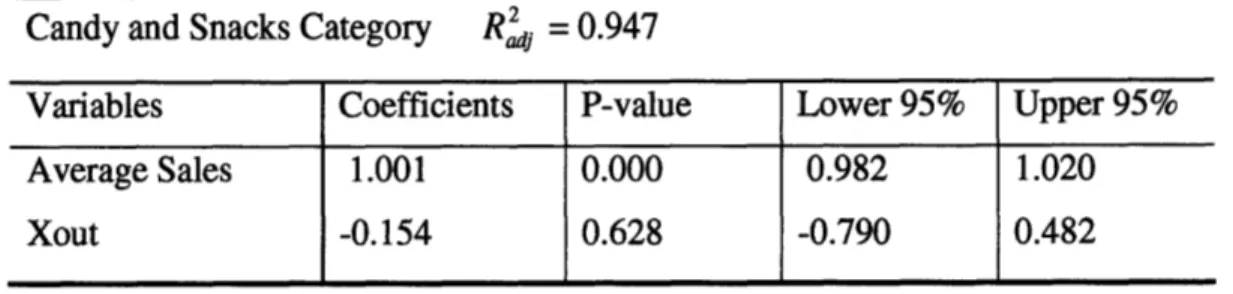
Candy and Snacks Category R' = 0.947
Variables Coefficients P-value Lower 95% Upper 95%
Average Sales 1.001 0.000 0.982 1.020
Xout -0.154 0.628 -0.790 0.482
Table 5: Regression model for category 'Candy and Snacks'
The coefficient for Xout variable in the 'Candy and Sancks' model did not turn out to be significant. For category of candy and snacks there is a downstream impact of 15.4 cents for each dollar in stock-out at the distribution center level. For this particular
category there was no promotional events in one year of data analyzed, hence the impact of promotions was not included.
The final category analyzed was for food, and the results for the food model are given in Table 6.
Food Category R4d = 0.939
Variable Coefficients P-value Lower 95% Upper 95%
Average Sales 0.989 0.000 0.932 1.046
Promotion Sales 0.199 0.105 -0.042 0.442
Table 6: Regression model for category 'Food'
From the regression results of the aggregate as well as the individual category models, we see that the stock-out at the distribution center does have a detrimental impact at the downstream store sales. However, in the individual category models the coefficient for the Xout variable is not significant at the 95 percent confidence level. The other impact
we see in these models is that the promotion events are causing the sales to go up by a magnitude which is different across the individual categories.
5
Data mining to Determine Drivers of Stock-out
This section summarizes the data analysis that has been performed using data mining techniques and the results and conclusions that have been obtained. Regression analysis and logit modeling techniques were used to determine the drivers of stock-out at the store level. Finally, data clustering approach was used to cluster together stores having similar attributes and store performance in terms of stock-outs. Analysis was performed on the good performance and the worst performance store clusters to determine what potential attributes would have caused that behavior.5.1
Drivers of Stock-out
-
Using Multiple OLS Regression
Regression analysis was carried out on the 8 high moving SKUs over one year history to determine the drivers of stock-outs. Before the modeling effort was done, correlation analysis was carried out on all the data attributes to determine the degree of correlation existing among them. While building predictive models, the effect of correlation among the variables does not affect the accuracy of the model but for explanatory models it is important to isolate variables which are highly correlated in order not to get any misleading indicators. The detailed correlation matrix for all the variables is given in Appendix B. The variables which were having a high correlation (above 0.5) are
summarized below:
* Stock-outs had a high correlation of 0.51 with inventory turns
* The correlation between Average inventory-on-hand (IOH) and Demand per week was 0.651
* Correlation between Inventory turns and Demand per week was -0.735
* Correlation between stores opened for 2 to 5 years and with a front-to-back layout was 0.579
After analysis of the correlation data, multiple regression models were built predicting the dependant variable of stock-out. More than 30 models were calibrated using different combination of variables to maximize the R2 while at the same time coming up with a
model that satisfies all the criteria for statistical significance. The final model that was chosen out of all the iterations is given in Table 7.
Regression model predicting drivers of Stock-out R' = 0.711
Category Variables Coefficients P-value Lower Upper
95% 95%
Inventory Average Inventory-on-hand (IOH) 0.112 0.000 0.086 0.138
Low-income area 2.376 0.000 1.974 2.778
Demographics Medium-income area 1.634 0.000 1.293 1.975
African-American population 0.694 0.006 0.191 1.198
Mon store-delivery 1.253 0.000 0.783 1.723
Tue store-delivery 1.101 0.000 0.683 1.519
Delivery Wed store-delivery 1.584 0.000 1.125 2.044
Thu store-delivery 1.233 0.000 0.756 1.712
Fri store-delivery 1.255 0.000 0.785 1.726
Store -Low square-footage 1.642 0.000 1.269 2.015 Store -Medium square-footage 1.622 0.000 1.318 1.927
Store Attributes Distance store-DC > 200 miles 1.205 0.000 0.883 1.528
Store opened less than 1 year 3.942 0.000 2.282 5.602
Store opened 1-2 years 1.545 0.000 0.783 2.307
Store opened 2-5 years 1.103 0.000 0.735 1.472
Table 7: Regression model giving the drivers of stock-out
The final regression model was selected based on high R2j and also the model as a
whole and the individual co-efficients were all significant at the 95 percent confidence level. The detailed output of this regression model is given in Appendix B. Variables that were not included in the final model are given below, along with the reasons why they were not included:
Inventory turns: Including inventory turns instead of average inventory-on-hand (IOH) did not work out because a number of variables in the model turned
insignificant at the 95 percent confidence level once it was included. Hence, inventory turns variable was excluded from the final model.
* Demand per store: Demand variable had a very high correlation (0.65) with the Average IOH, and hence was not included in the model.
* DC dummy variables: Including the DC variables such as Alachua, Scottsville, Fulton etc. indicating which DC the store was being replenished from did not improve the R2 of the model and caused some of the variables to become insignificant at the 95 percent confidence level. Therefore, the DC variables were not included in the final model.
* Store layout variables: Store layout variables (Racetrack, FTP, Market, Flipped and traditional) were not included in the final model as well because after including these variables, the coefficients were not significant at the 95 percent confidence level.
Results and Conclusion
Based on the interpretation of the final regression model we can draw the following insights about the stock-out performance of stores:
Income of the area (Low-income, medium-income, high-income): Low income
areas were categorized where the average annual income was less than 30,000 (25t
percentile) and medium income areas with income between 30,000 and 46,000. Areas with average annual income higher than 46,000 (75t percentile) was categorized as high income areas. Average income of the area in which the stores are located is a significant explanatory variable for the stock-outs at the store-level.
If a store is located in a low income area it has on average 2.37 more stock-outs per week (for the 8 high moving SKUs) than a store located in a high income area. Similarly, a store located in a medium income area on average has 1.63 stock-outs per week more than a store located in a high income area.
* Demographic variables (African-American areas): If a store is located in a
pre-dominantly African-American neighborhood (greater than 50 percent of the population) it will have higher chances of stock-outs. The empirical results show that on average the retail stores in that region will have 0.69 stock-outs per week more than a store which is not in an American neighborhood. The African-American and Low-income variables are positively correlated by 0.28, and because of this these neighborhoods will have more low-income areas as well.
* Store size (Low sq-footage, Medium sq-footage, High sq-footage): The final model
shows that store size has an impact on the average stock-outs. Stores were
categorized in three size categories: Low sq-footage (less than 7300 sq-ft), medium sq-footage (7300 - 9500 sq-ft) and high sq-footage (greater than 9500 sq ft). If a store has a smaller square footage it will have an average of 1.64 stock-outs per week more than a store which has a high sq-footage. Similarly, if a store has a medium square footage it will have 1.2 stock-outs per week more than a store which has a high square footage, all else being equal.
* Distance of storefrom distribution center (greater than 200 miles): Distance of
store from the distribution center came out to be a significant explanatory variable. If the distance of the store from the distribution center is greater than 200 miles, that store will have on the average 1.2 more stock-outs than a store within 200
miles of the distribution center. Greater distance from the distribution center would pose more logistical challenges in store replenishment and cause worse stock-out performance.
* Number of years the store has been in operation (Less than I year, 1-2 years, 2-5
years, >5 years): Age of the store is another determinant of the stock-out
performance of the store. The newer a store is, the higher stock-outs it tends to have. If a store has been opened for less than a year, it will have 3.94 stock-outs more than a store which is in operation for more than 5 years. Similarly, a store which has been in operation for 1 to 2 years will have 1.54 more stock-outs and a store which has been in operation for 2 to 5 years will have 1.1 more stock-outs than a store which has been operating for more than 5 years.
Demand variability in newer stores could be a possible reason for better stock-out performance of older stores. To determine this, I analyzed the coefficient of variation of demand for the stores by the number of years they have been in operations. It is concluded from the graph below that demand variability is not very different based on the age of the stores, and the contributing factors could be the management and store practices which causes higher stock-outs for new stores. Newer stores will have less experienced store managers and staff and this could potentially cause higher stock-outs due to shelf-replenishment issues.
Co-efficient of variation for Demand for Stores
Figure 7: Demand variability for stores by number of years the stores have been in operation.
Day of the week delivery: Day of the week delivery does not predict a significant pattern for delivery days which would cause higher stock-outs. Although from the model coefficients itself, Wed delivery is the one which causes the maximum stock-outs relative to other days' delivery and Sunday delivery has the minimum stock-outs.
5.2
Drivers of Stock-out
-
Using Logistic Regression
Logistic regression was performed over one year history at a store/SKU/week level. The correlation analysis was used as a guide for including the variables in the logit models, so that independent variables with significant correlation are not included in the model. Including highly correlated variables in the model could reduce explanatory power of the model and can give biased insight into the impact of the independent variables. The dependent variable was a binary stock-out variable (1 or 0) - 1 being if there was a
stock-0.30 = 0.25 " 0.20 o 0.15 Q 0.10 0.05 0.00 1-2 Years 2-5 Years Store Operation -
--Less than 1 year
I
out for the particular SKU for that week for the store, and 0 being if there was no stock-out. The pre-processed volume of the data was around 1.5 million data points on which logistic regression was performed using SAS software.
More than 15 logit models were calibrated with different combination of variables to come up with the best model. In logit models, the likelihood ratio is used as the criterion for a good model and also all the variables are checked for statistical significance. The final model that I obtained is given below in Table 8.
Logit model predicting drivers of Stock-out Likelihood Ratio = 2933
Category Variables Coefficients P-value Lower Upper
95% 95%
Intercept -2.872 0.000 -2.942 -2.802
Inventory Average Inv-on-hand (IOH) -0.043 0.000 -0.047 -0.039
Demographics Low-income area 0.124 0.000 0.102 0.146
African-American population 0.342 0.000 0.311 0.376 Store -Low square-footage -0.051 0.000 -0.078 -0.021 Store - Medium square-footage -0.035 0.004 -0.059 -0.011 Distance store-DC > 200 miles 0.206 0.000 0.184 0.228
Store Attributes Store opened less than 1 year 1.652 0.000 1.563 1.741
Store opened 1-2 years 0.191 0.000 0.134 0.248 Store opened 2-5 years 0.085 0.000 0.059 0.111 Store layout-Racetrack -0.363 0.000 -0.435 -0.291
Store layout-Market -0.315 0.000 -0.436 -0.194
Table 8: Logistic Regression model giving the drivers of stock-out
Some of the variables were not included in the final model due to the reasons given below:
* Inventory turns: Including inventory turns in the model instead of average
inventory-on-hand (IOH) changed some of the other variables as insignificant, and was not included.
* Demand per store: Demand had a high correlation with average IOH and since inventory-on-hand was included, demand was not included in the model. * Day of the week delivery: Including day of the week delivery caused two of the
variables (Wed and Fri) to be not significant at the 95 percent confidence level. Therefore, day of the week delivery variables were not included in the model. * Income and store layout variables: Variable for medium income and store layout
variables FTB (front-to-back) and flipped were not significant at the 95 percent confidence level and were not included. The final model included the categorical variable of low income.
The interpretation of the logistic regression coefficients is, however, a bit more
complicated than an ordinary-least-squares (OLS) regression. It is useful to give the odds ratio estimates for the parameters which give an insight into the sensitivity of the model. For example, the odds ratio estimate for the categorical variable Low-Income is 1.132 (which is exponent of 0.1244). The odd ratio estimate predicts how the probability of stock-out will change given a change in one of the independent variables. For Low-income variable, if the store is in a low income area, the probability of stock-out would be 1.132 times (or 13.2 percent) higher than if the store were not in a low income area. The odds ratio estimates for the coefficients of the logistic regression model are given in Table 9.
Odds Ratio estimates for logit coefficients
Category Variables Point Lower Upper
Estimate 95% 95%
Inventory Average Inv-on-hand (IOH) 0.958 0.954 0.962
Low-income area 1.132 1.108 1.157
Demographics African-American population 1.408 1.365 1.455
Store low square-footage 0.951 0.924 0.978 Store Medium square-footage 0.966 0.943 0.989 Distance store-DC > 200 miles 1.229 1.202 1.256
Store Attributes Store opened less than 1 year 5.218 4.782 5.695
Store opened 1-2 years 1.210 1.144 1.280 Store opened 2-5 years 1.089 1.061 1.117 Store layout-Racetrack 0.696 0.648 0.746
Store layout-Market 0.730 0.648 0.822
Table 9: Odds ratio estimates for logistic regression model.
Results and Conclusion
Based on the odds ratio estimates of the logistic regression model, we can obtain the following insights about the drivers of stock-out for retail stores:
Average Inventory-on-Hand (IOH): The model predicts that the probability of
stock-outs becomes lower if the average inventory-on-hand (IOH) increases. For every one unit increase in the average inventory-on-hand, the probability of stock-out becomes 0.958 (or a 4.2 percent reduction) of the prior probability. If the average IOH increases by 5 units, then the probability of stock-out becomes 0.806 (or 19.3 percent lower) than before. This result is intuitive, because more inventory on hand will provide a higher buffer/safety stock against stock-outs. However,
there are cost implications of raising the inventory levels in the supply chain as well.
* Income of the area (Low-income area): If the store is in a low income area, the
probability of stock-out would be 1.132 times higher than if it were not in a low-income area. Low low-income areas could have less experienced store management and staff which can cause worse stock-out performance.
* Demographic variables (African-American area): The model predicts that if a store
is in a pre-dominantly African-American neighborhood it will have a higher chance of stock-outs, and these finding are in line with the previous modeling effort with multiple regressions at the store-level. The model predicts that the probability of a stock-out will increase by 14 percent if the store is in an African-American
neighborhood.
* Store size (Low sq- footage, Medium sq-footage, High sq-footage): The logit model
predicts that store size has an impact on the probability of stock-out. If a store has low square-footage, the probability of stock-out is 0.951 times (or 4.9 percent less) than the probability if the store had a high square-footage. Similarly, if a store has medium square-footage, the probability of stock-out is 0.966 times (or 3.4 percent less) than the probability if the store had a high square-footage. In a study
conducted by Angerer (2005), it was discovered that bigger stores having larger backrooms typically face more challenges in terms of stock-out performance due to replenishment issues. The graph below highlights the impact of backroom size on out-of-stock (OOS) levels. The results from the logit model obtained depict a similar trend with store size as well.
Figure 8: Impact of backroom size on stock-out levels. (Source: The Impact of Automatic Store Replenishment Systems on Retail. Alfred Angerer, 2005)
* Distance of store from distribution center (greater than 200 miles): The model predicts that if that if the distance of the store from the distribution center was greater than 200 miles, the probability of stock-out will be higher. In empirical terms, if the store is more than 200 miles from distribution center, the probability of stock-out will be 1.229 times (or 22.9 percent higher) than if the store was less than 200 miles from the distribution center. This insight is intuitive as well, because the further the store is from the distribution center it will face greater logistical
challenges in replenishment.
* Number of years the store has been in operation (Less than I year, 1-2 years, 2-5 years, >5 years): Number of years the store has been in operation is another determinant of the stock-out performance of the store. The model gives the insight that newer stores have higher probability of stock-out. According to the logit odds
14 -p4
OOS UPt
0A
Bko Fm~ei Fme Se iQq ITers 4,)
8dWOOM ý-Melefs'
shlei fe
Sq
eens
1;Mj
ratio estimates, if a store has been opened for less than a year, its probability of stock-out will be 5.218 times higher than if the store had been in operation for more than 5 years. For stores that have been in operation for 1-2 years and 2-5 years, the probability of stock-out is 1.210 and 1.089 times higher respectively, than if the store had been in operation for 5 years or more. The model gives the insight that stores which have been in operation for less than one year are particularly
susceptible to bad performance and higher stock-outs.
Store Layouts: The model gives some insight into store layouts. It predicts that if a
store has Racetrack4 layout, the probability of stock-out is 0.696 (or 30.4%
reduction) times the probability if it was traditional, front-to-back or flipped layout. This could be due to the ease of shelf-replenishment in the race-track layout where the aisles are visible to store staff and stock-out situations could be handled more effectively. Similarly, if the store has a market layout, the probability of stock-out is 0.73 times (or 27% less) the probability of stock-out if it was traditional, front-to-back (FTB) or flipped layout.
5.3
Data Clustering Approach
There are two primary data clustering mechanisms in data mining: hierarchical clustering and non-hierarchical clustering. For my research, I have primarily used non-hierarchical clustering techniques using k-means algorithm. Although I also used hierarchical data clustering in the research and the approach was giving similar results to the
non-hierarchical methods. K-means algorithm is a fast and efficient means of clustering data 4 'Racetrack' layout is a newer layout for RetailerCo with merchandise arranged in a racetrack fashion with
and was used for the purpose of my research. The overall approach was to form clusters which would have similar attributes in terms of store characteristics and stock-out performance and then further analyze the good or bad store clusters to determine the common attributes among these clusters.
The first step in data clustering is to normalize the data by bringing the data from different attributes on a common scale so that they can be comparable to each other. Normalization is accomplished by subtracting the mean from the data point and dividing
by the standard deviation to convert it into standard z-score (x - /). After the data
normalization was completed on 16 different attributes and 4046 stores, k-means algorithm was used to perform data clustering. Data clustering was done using different number of clusters to achieve the best possible clustering scenario which had distinct clusters of good and bad performance stores. I started the clustering exercise with 2 clusters and gradually increased the number of clusters. Once the number of clusters was small, there were no distinct clusters which had measurements of stock-outs lower or higher than average which could be classified as good or worse performing clusters. As I increased the number of clusters, I was able to obtain some clusters which were different from the rest of the
population in terms of stock-out performance. Through this iterative process, I selected the final clustering scheme which had 10 clusters in it.
The final clustering scheme is given in Table 10, with the number of stores falling in each cluster. The table also gives the average distance in cluster which is the average Euclidean distance from the centroid of each cluster to each data point in the cluster. The
Cluster no. No of Stores Percent Stores Average Distance in cluster Cluster-1 952 23.5% 1.851 Cluster-2 254 6.3% 1.958 Cluster-3 31 0.8% 5.580 Cluster-4 141 3.5% 1.952 Cluster-5 424 10.5% 2.084 Cluster-6 353 8.7% 2.016 Cluster-7 854 20.8% 1.610 Cluster-8 219 5.4% 1.721 Cluster-9 389 9.6% 2.354 Cluster-10 443 10.9% 2.051
Table 10: Data clustering summary for 10-clusters.
After forming data clusters based on the data attributes, statistics on store stock-out performance were calculated. Figure 9 gives the average stock-outs for all the stores and compares it against the average stock-outs for the individual clusters formed.
Average Stock-out for clusters of Stores
Bad performance clusters
12 -10 - 8- 6- 4- 2-
0-Average for all stores
(,,
Good performance clusters
ztL
- 1- Is..a
3--Figure 9: Stock-out performance of all stores vs. clusters of stores
A
--Cluster no. No of Average Stock-out relative to Stores average of all stores
Good performance Clusters:
Cluster-5 424 64% lower
Cluster-4 141 59% lower
Cluster-8 219 54% lower
Worst performance Clusters:
Cluster-9 389 62% higher
Cluster-10 443 72% higher
Table 11: Stock-out performance of good and worst performance clusters relative to average for all the stores.
Cluster-5, Cluster-4 and Cluster-8 can be categorized as the store clusters having better stock-out performance on average and Cluster-9 and Cluster-10 can be categorized as the cluster of worst-performing stores. These clusters have been formed not just on the basis of stock-outs but the rest of the store attributes including day of delivery,
demographic variables, income in area, distance metric from store to distribution center, square footage of stores, number of years store has been in operation and layout of the store.
Results and Conclusion
After segregating stores into good and worst performance clusters, further analysis was carried out on Cluster-9, Cluster-10 (worst performing clusters) and Cluster-5, Cluster-4 and Cluster-8 (good performance clusters) to gain further insight into the drivers of better or worse than average stock-out performance.
Worst-Performing Store Clusters:
Store Clusters 9 and 10 were analyzed to determine the drivers which are causing a higher stock-out for these stores. Table 12 gives the different attributes of 9 and
Cluster-10 compared to the overall statistics for the whole population. T-tests were performed at 99 percent confidence level to determine if the cluster mean for a particular attribute was different than the population mean for that attribute. In Table 12, the attributes and P-value of clusters which are bolded indicate that at 99% confidence level the cluster mean for the particular attribute is different from the population (all stores) mean. This would help establish which attributes of the cluster are the differentiating factors from the overall population of stores which is causing bad stock-out performance.
Cluster Attribute Average IOH Average Income African-American Mon-delivery Tue-delivery Wed-delivery Thu-delivery Fri-delivery Sun-delivery Square-footage Stores-Years in operation Distance > 200 miles Layout: Racetrack Layout: Front-to-back Layout: Market Layout: Flipped Layout: Traditional
Av. for all stores 16.5 37,011 8.0% 14.9% 25.5% 16.2% 13.9% 15.2% 14.2% 8,705 11.21 21.0% 2.4% 23.3% 1.0% 3.8% 69.5% Cluster-9 (Low-Income, Newer) 16.8 31,068 12.3% 11.1% 19.8% 19.5% 17.2% 15.2% 17.2% 11,496 9.05 22.9% 5.9% 22.1% 4.1% 4.1% 63.7% T-test P-value (2-tailed) 0.055 0.000 0.012 0.024 0.007 0.116 0.100 0.975 0.131 0.000 0.000 0.407 0.004 0.102 0.002 0.752 0.024
(Newer, further from
DC)
15.1 39,940 3.6% 43.6% 4.5% 16.5% 10.4% 11.7% 13.3% 8,177 8.28 56.9% 2.9% 37.0% 0.2% 5.4% 54.0% t-Test P-value (2-tailed) 0.000 0.000 0.000 0.000 0.000 0.897 0.022 0.033 0.600 0.000 0.000 0.000 0.521 0.000 0.003 0.144 0.000Table 12: Comparison of attributes of worst performing clusters vs. overall store population