HAL Id: hal-03047964
https://hal.sorbonne-universite.fr/hal-03047964
Submitted on 9 Dec 2020
HAL is a multi-disciplinary open access
archive for the deposit and dissemination of
sci-entific research documents, whether they are
pub-lished or not. The documents may come from
teaching and research institutions in France or
abroad, or from public or private research centers.
L’archive ouverte pluridisciplinaire HAL, est
destinée au dépôt et à la diffusion de documents
scientifiques de niveau recherche, publiés ou non,
émanant des établissements d’enseignement et de
recherche français ou étrangers, des laboratoires
publics ou privés.
Tip growth in morpho-elasticity
Martine Amar, Julien Dervaux
To cite this version:
Martine Amar, Julien Dervaux. Tip growth in morpho-elasticity. Comptes Rendus Mécanique,
Else-vier Masson, 2020, 348 (6-7), pp.613-625. �10.5802/crmeca.27>�. �hal-03047964�
Comptes Rendus
Mécanique
Martine Ben Amar and Julien Dervaux
Tip growth in morpho-elasticity
Volume 348, issue 6-7 (2020), p. 613-625. <https://doi.org/10.5802/crmeca.27>
Part of the Thematic Issue: Tribute to an exemplary man: Yves Couder
Guest editors: Martine Ben Amar (Paris Sciences & Lettres, LPENS, Paris, France),
Laurent Limat (Paris-Diderot University, CNRS, MSC, Paris, France), Olivier Pouliquen (Aix-Marseille Université, CNRS, IUSTI, Marseille, France) and Emmanuel Villermaux (Aix-Marseille Université, CNRS, Centrale Marseille, IRPHE, Marseille, France)
© Académie des sciences, Paris and the authors, 2020.
Some rights reserved.
This article is licensed under the
Creative Commons Attribution 4.0 International License.
http://creativecommons.org/licenses/by/4.0/
LesComptes Rendus. Mécanique sont membres du Centre Mersenne pour l’édition scientifique ouverte
Comptes Rendus
Mécanique
2020, 348, n 6-7, p. 613-625
https://doi.org/10.5802/crmeca.27
Tribute to an exemplary man: Yves Couder
Morphogenesis, elasticity / Morphogenesis, elasticity
Tip growth in morpho-elasticity
Martine Ben Amar
∗, a, band Julien Dervaux
caLaboratoire de Physique de l’Ecole normale supérieure, ENS, Université PSL, CNRS,
Sorbonne Université, Université de Paris, F-75005 Paris, France
bInstitut Universitaire de Cancérologie, Faculté de médecine, Sorbonne Université,
91 Bd de l’Hôpital, 75013 Paris, France
cLaboratoire Matière et Systèmes Complexes, UMR 7057, CNRS and Université de
Paris, 75013 Paris, France
E-mails: [email protected] (M. Ben Amar),
[email protected] (J. Dervaux)
Abstract. Growth of living species generates stresses which ultimately design their shapes. As a consequence,
complex shapes, that everybody can observe, remain difficult to predict, even when the growth biology is over-simplified. One way to tackle this question consists in limiting ourselves to quasi-planar objects like leaves in the spring. However, even in this case the diversity of shapes is really vast. Here, we focus on growing tips with the aim to compare their role in elastic growth to classical viscous fingering and dendritic growth. With the help of complex analysis, we show that a parabola under constant growth is free of stress while growing but any growth perturbation will strongly affect its final shape. Two models of finite elasticity are considered: the Neo-Hookean and the poro-elastic model with incompressibility.
Résumé. La croissance biologique génère des contraintes mécaniques qui contribuent à façonner la forme
des tissus, des organes et des organismes vivants. En raison de l’extrême complexité des phénomènes de croissance biologique, il est en général impossible de prédire ces formes. Dans certains cas géométriquement simples, par exemple des tissus biologiques minces en croissance quasi-planaire tels que des feuilles, les lois de la mécanique contraignent les formes possibles. Toutefois, l’espace des formes atteignables reste particulièrement vaste. Dans ce compte-rendu, nous nous intéressons au cas particulier des pointes en croissance, que nous décrivons dans le cadre de la théorie de la morpho-élasticité et de la poro-élasticité non-linéaire, et qui partage des similarités frappantes avec deux sujets d’étude classiques en physique : la croissance dendritique et la digitation visqueuse. Les outils de l’analyse complexe sont mobilisés pour montrer qu’une parabole en croissance homogène est stable et ne développe pas de contrainte mécanique. En revanche, la forme de la pointe est fortement affectée par les perturbations du champ de croissance.
Keywords. Nonlinear elasticity, Biological growth, Instabilities, Morphogenesis, Meristem growth.
∗Corresponding author.
1. Introduction
Morphogenesis is the biological process by which living organisms acquire their shape. While biological growth is mostly under the control of genetics, the set of possible shapes of biological objects is ultimately constrained by physical principles. At a cellular scale, growth and division can be described by local, time-dependent, laws. However, integrating such local laws in order to explain the (possibly evolving) shapes of macroscopic objects (leaves, flowers, trees, organs, tumors, biofilms, etc.) is a formidable task. If we limit ourselves to botanics, which is simpler in the sense that growth is less constrained by boundary conditions, and even if we further restrict ourselves to leaves because of their geometric simplicity, a broad diversity appears in nature that perhaps physics and mechanics may help to understand or at least to classify.
Upon observing the growing leaves of trees in spring, one may first notice that some leaves are mostly planar, in particular when the ribs are not too thick compared to the leaf thickness. When this is not the case, the leaf typically buckles between two successive ribs and the differential growth leads to sharp pointed tips, one being along the symmetry axis of the leaf with the others organized on both sides, as observed on holly leaves. But for thin leaves and tiny ribs, on the other hand, the membrane remains planar and the outer contour is smooth, with either regular or undulated boundaries depending on species.
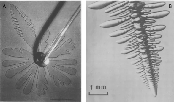
Tip instabilities of growing inert matter are also frequently observed. Archetypal examples of “growing” systems exhibiting morphological instabilities in physics are dendritic (diffusive) growth and radial viscous fingering [1, 2], illustrated in Figure 1. Of course, unlike biological growth, there is no creation of matter in these classical experiments but rather a displacement of a material into an another one. Two broad classes of instabilities in these systems have been documented: tip splitting in viscous fingering and side-branching in diffusive out-of-equilibrium processes. Due to the nonlocal nature of the “growth” processes, ie the competition between surface tension and a diffusive or Laplacian field, understanding these patterns turned out to be a real challenge and both of these topics have been the subject of a considerable amount of experimental, numerical, mathematical and theoretical work in the past forty years.
A naive idea to explain the predominance of side-branching events in dendrite growth and of tip-splitting instabilities in viscous fingering lies on the difference between Laplacian and diffu-sional fields. Dendrite tips in diffusive systems preserve their size to maintain stabilization by sur-face tension while growing Laplacian fingers in open geometries keep growing and thus must di-vide in order to maintain stability by surface tension. This sharp separation of physical processes can be somewhat perturbed by the addition of a localized perturbation. As demonstrated by Yves Couder and his collaborators, trapping of a small bubble at the tip of a growing viscous finger re-sults in a stable finger growing at constant velocity and emitting dendrite-like sidebranches [3–5]. The emergence of a theoretical framework coupling biomechanics to growth in the last years now offers a unique way to understand problems of morphogenesis and embryogenesis where the biology at small scales is strongly coupled to biomechanics, and elasticity, see in particu-lar [6, 7]. By analogy with some of his favorite hydrodynamic instabilities, namely crystal growth and viscous fingering, Yves Couder has suggested some universality in growth patterns poten-tially dominated by leading growing tips, in particular in botany. More precisely, he suggested that growing tips, described within the formalism of morpho-elasticity, might share some char-acteristics with Laplacian or diffusive growth. The aim of this paper is thus to scrutinize carefully this hypothesis. Let us stress however, that it took fifty years to understand Laplacian [8] or den-dritic growth [9] following the first pioneering works of respectively Saffman and Taylor [10] and Ivantsov [11] and unfortunately, the mathematics of finite or nonlinear elasticity is much more complex than that of diffusive or Laplacian growth. As a consequence, our modest contribution will be limited to the simple case of a parabola under: (i) constant volumetric growth, isotropic
Martine Ben Amar and Julien Dervaux 615
Figure 1. On the left, viscous fingering in an open geometry. The anomalous dendritic
finger is due to a pulsating tip. The image is reproduced from Couder, Y., Cardoso, O., Dupuy, D., Tavernier, P. and Thom, W. [3]. On the right, a dendrite of succinonitrile growing in an undercooled melt, exhibiting the characteristic paraboloidal tip and the secondary sidebranching behind the tip. The figure is reproduced from J. S. Langer [4].
or slightly anisotropic and (ii) homogeneous poro-elastic swelling and (iii) to the existence of un-dulating modes at the leave borders.
2. Finite-Elasticity in complex geometry
The basis of elasticity dates at least from the 17th-century with the first statement De Potentia
Restitutiva of Robert Hooke (1678), but any application of the first principles remains
challeng-ing in bodies of non trivial shapes and of finite size [12]. Indeed, if we really want to analyze the field of deformations of a specific body under an external loading, we are faced to its geomet-rical description. It is why, in textbooks, examples are restricted to bars, spheres, cylindgeomet-rical or spherical shells. This challenge is even increased in non-linear elasticity [13–15] since we need to consider both the initial and the final geometries or initial and final configurations. This explains why, only simple geometries have been considered since not only the shape is important but also the writing of equilibrium equations (density of forces and torques or Euler–Lagrange equations) in a more or less standard coordinate systems. As for living systems which to some extent, can be considered as soft elastic tissues, their shapes are much more diverse and also their elastic prop-erties. In addition, it exists strong differences between living and inert matter, the most obvious one being the ability to grow with specific rules. This induces stresses that need to be combined to loading or to other constrains, as the boundary conditions for example.
Keeping the strategies that many have followed for viscous fingering and dendritic growth, that is to focus on growing tips, we consider this shape which has been completely discarded in the context of volumetric growth. Tips are present in nature as the ends of branches, leaves, blades. We restrict on planar or quasi-planar objects to maintain plane strain elasticity. The
advantage of this geometry is a simple expression with holomorphic functions for borders, a simple way to construct a curvilinear system of coordinates where the initial shape turns out to correspond to one coordinate and finally a simple writing of the equations of non-linear elasticity with growth, as shown in the following. Adopting the technique of needle-crystals which have been assimilated to parabola or paraboloid, discarding side-branchings, we perform the elastic treatment in parabolic coordinates [16, 17].
2.1. Elasticity in parabolic coordinates
We consider a growing parabolic tip and write all the relevant equations of finite elasticity with growth [15] in the parabolic system of coordinates based on the conformal mapping of the (X , Y ) plane:
Z = X + I Y = −I
2((µ + Iη)
2
+ 1) = ηµ + I /2(η2− µ2− 1). (1) If the coordinateη is fixed to one, we derive the following relationships: X = µ and Y = −12X2
which represent a parabola of radius of curvature equal to unity (R = 1), oriented symmetrically along the negative Y axis. Here after, we choose as unit of length this radius of curvature.µ and η are orthogonal coordinates with a scale factor hµequal to |∂µR|, where ~~ R = X~eX+ Y ~eY, and the
equivalent definition for hη. In the following, we will adopt arbitrarily either the notation∂/∂α or the notation∂αfor the partial derivative with respect toα. hηand hµare the classical notations for changes of coordinate systems, see Morse and Feshbach’s book [18]) and for the parabolic coordinate defined by (1), we easily derive hµ= hη=pη2+ µ2. Considering that Z is the complex
coordinate in the configuration of reference and z in the current configuration, the geometric strain F and the elastic strain Fe (after conformal mapping transformation of coordinates) are
then: F = 1 h2 µ · ∂µx∂ηx ∂µy ∂ηy ¸ and Fe= 1 h2 µ · ∂µx/gµ∂ηx/gη ∂µy/gµ∂ηy/gη ¸ (2) where gµ and gη are the eigenvalues of a growth tensor, diagonal in the parabolic system of coordinates, possibly anisotropic when gµ6= gη. To simplify, these eigenvalues will be chosen independent of space coordinates but they can be dependent on time if the typical time-scale of growth is long compared to any dissipation process. We choose the simplest model of finite elasticity, the Neo-Hookean modelling [13–15] , and we assume incompressibility so:
Det Fe= 1 and DetF = gµgη soJ = ∂µx∂ηy − ∂ηx∂µy − hµ2gµgη= 0. (3) The elastic energy of the initially growing parabola is then:
E = E 2τ Z ˜ V dµdη{(∂µx)2+ (∂µy)2+ τ2{(∂ηx)2+ (∂ηy)2} − 2hµ2gµ2− 2pJ } (4) where E is the shear modulus and p is the Lagrange multiplier which allows to impose the incompressibility constraint. A priori, p is a function of bothµ and η. The coefficient of anisotropy is given byτ = gµ/gη. We can eliminate the anisotropy coefficient by dilating the variable µ = τν but the price to pay is the change of the scaling factors hµ. Indeed, we must reminder that h is a function ofµ and η so only when h depends on a unique coordinate, the anisotropic case can be treated as the isotropic one (this is the case of the cylindrical or radial geometry). If not, we are really constrained. In this curvilinear coordinate system, the Euler–Lagrange equations read:
∆η,µx =∂ 2x ∂µ2+ τ 2∂2x ∂η2= ∂p ∂µ ∂y ∂η− ∂p ∂η ∂y ∂µ ∆η,µy =∂ 2y ∂µ2+ τ 2∂2y ∂η2= − ∂p ∂µ ∂x ∂η+ ∂p ∂η ∂x ∂µ. (5)
Martine Ben Amar and Julien Dervaux 617
One can notice that (5) are similar to the same equations for the growth of a sample in a stripe, written in cartesian coordinates. If the choice is made of holomorphic function for x and y and for isotropic growth,τ = 1, the Lagrange parameter p is a constant. Because of the incompressibility constraint, our choice for the deformation will be in favor of a solution which restores the parabolic shape. So we hypothesize:
x = λxηµ and y =
λy
2 (η
2
− µ2− 1). (6)
The Jacobian of the new configuration is then J = λxλy·(η2+µ2) = λxλyhµ2so the
incompressibil-ity condition imposesλxλy= gη2τ, according to (3). But we one cannot verify the second Euler–
Lagrange equation for y and new guess of possible solution is not so easy to find. It is why we choose first the isotropic case withτ = 1, ∆µ,ηx = ∆µ,ηy = 0 and the pressure p constant and opt
for a weak anisotropic perturbation. So, our exact result is limited to isotropic growth and weak perturbed elastic fields will be evaluated once driven by weakly anisotropic growth. Boundary conditions forη = 1 concern the cancellation of the two components of the nominal stress:
Sη,η= E µ τ2∂y ∂η− p ∂x ∂µ ¶ and Sη,µ= E µ τ2∂x ∂η+ p ∂y ∂µ ¶ (7) which gives: p = 1 and λy= λx= gη= g . So finally a parabola which grows isotropically enlarges during development and its radius of curvatureR is simply the growth factor g. This solution differs from the initial configuration. If g > 1, the parabola seems smoother than the initial one while if g < 1, it appears more sharp-pointed. Since this constant homogeneous growth process does not generate any kind of stress, the parabolic shape is stable and no shape bifurcation is then expected, contrary to the growth of a layer [19, 20]. In the next section, we confirm that the parabola, with constant isotropic growth, is a robust shape and that deviation from this shape will require a change in the growth conditions.
3. Variations around the stress-free parabola
The stress-free parabola found previously is an exact solution of the elasto-static growth problem. To find exact solutions, even in the Neo-Hookean approach remains a challenge but it remains possible to slightly perturb the growth conditions. Considering anisotropic growth, the weakness is represented by the small coefficient ² = τ − 1 where τ intervenes in (4), (5), (7). We will use this parameter to expand linearly the main equations.
3.1. Weakly anisotropic growth
At linear order in², x, y, p and J are transformed into: x = g (ηµ + ²u(µ,η)) y =g 2(η 2 − µ2− 1) + ²g v(µ, η) p = 1 + ²π(µ,η) J = g2(η2 + µ2) + ²j (µ,η) − g2τ(η2+ µ2). (8) For j (µ,η), it reads: µ µ∂u ∂η− ∂v ∂µ ¶ + η µ∂v ∂η+ ∂u ∂µ ¶ = a0(η2+ µ2) (9)
where a0is equal to 1 ifτ 6= 1 and is zero for the isotropic case, τ = 1.
that we can transform into: ∂u ∂η− ∂v ∂µ= ηm(µ, η) + a0µ ∂v ∂η+ ∂u ∂µ= −µm(µ, η) + a0η (10)
where m(µ,η) is an arbitrary function. Notice that m = 0 means that (u,v) are complex conjugates since they verify the Cauchy relations. Deriving the first equation of (10) with respect toη and the second equation with respect toµ and adding both results gives:
∆u = η∂m
∂η − µ ∂m
∂µ (11)
and the same operation consisting in taking first the derivation with respect toµ, then with respect toη gives after substraction:
∆v = −η∂m
∂µ − µ ∂m
∂η. (12)
These two relationships have to be compared to the linear version of (5) which gives: ∆u = µ η∂π ∂µ+ µ ∂π ∂η ¶ (13) ∆v + 2a0= µ −µ∂π ∂µ+ η ∂π ∂η ¶ . (14) So we relateπ to m: ∂π ∂µ= ∂m ∂η − 2a0µ η2+ µ2 and ∂π ∂η= − ∂m ∂µ + 2a0η η2+ µ2 (15)
π satisfies the Poisson equation:
∆π = 4a0 µ 2
− η2
(η2+ µ2)2. (16)
The general solution for u and v can be found more easily if we combine both (41) and (42) and define U = u + I v
∆U = −2Idπ
d ¯ζζ − 2I a0 whereζ = µ + Iη (17)
π is a real function which can be decomposed into an holomorphic one P(ζ) and a contribution
due to the anisotropy. It is easy to show that
π =1 2 µ P (ζ) + ¯P ( ¯ζ) − a0 µζ ¯ ζ+ ¯ ζ ζ ¶¶ (18) and one easily find that
∂2U ∂ζ∂¯ζ= −I /4 µ d ¯P ( ¯ζ) d ¯ζ ζ + a0 µ 1 +ζ 2 ¯ ζ2 ¶¶ . (19)
Before going further, let us remind the boundary conditions: first symmetry along the X axis:
x = U (µ,η) = 0 and ∂µx = 0 = ∂µU = 0 for η = 0, second cancellation of the stresses Sη,µand Sη,η
forη = 1, see (7). Let us first consider linear perturbation of the stresses: Σ(µ,η) = Sµ,η+ I Sη,η= −2I∂U
∂¯ζ− πζ + 2a0ζ = 0 for η = 1,∀µ. (20)
Integrating (19) with respect toζ, we obtain:
∂U ∂¯ζ = − I 8 µ d ¯P ( ¯ζ) d ¯ζ ζ 2 + 2a0 µ ζ + ζ 3 3 ¯ζ2 ¶¶ +Q0( ¯ζ) (21)
Martine Ben Amar and Julien Dervaux 619
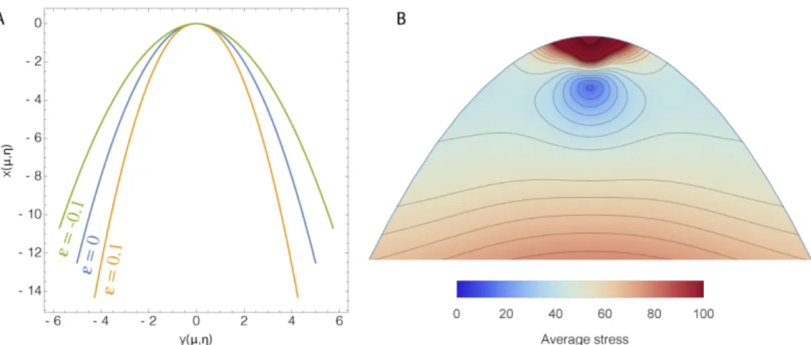
Figure 2. On left, quasi parabolic shapes for anisotropic growth. In blue, the growing
parabola with² = 0 (isotropic growth), in green the perturbed shape with ² = −0.1, in orange similar result with² = 0.1. ² ≥ 0 means that the growth factor along µ is larger than along
η. All lengths are scaled by the growth coefficient g. On right,qΣi , jS2i j (with i < j ) average
stress density inside the parabolic shape. Notice the divergence of the stresses near the tip:
µ ∼ 0, η ∼ 0.
Q( ¯ζ) can be evaluated once introduced in the stress function, Equation (20), which vanishes for η = 1 so for ζ = ¯ζ + 2I. So we get:
Q( ¯ζ) =1 6 µ −4/ ¯ζ + 12 ¯ζ −7I 2 ¯ ζ2¶. (22)
Finally, U will be fully determined by integrating (21) imposing u = 0 = ∂µu = 0 for η = 0 and
imposing also convergence whenµ− > ±∞. Then, the profile function becomes, under weakly anisotropic growth: x = g ηµ ½ 1 + ² µ −32+23 η 2 µ2+ η2 ¶¾ y =g 2 ½µ 1 +3² 2 ¶ (η2− µ2− 1) +34² 3 − 2²η µ 4 + η −2 3 η3 − 2 η2+ µ2 ¶¾ (23)
where² = τ − 1 = gµ/gη. So anisotropic growth reduces the radius of curvature of the parabola when gµ> gηas shown in Figure 2 on left. One also notices on right that the stresses diverges at the tip which seems unphysical. This explains that the real tip requires a modification of the growth law or a change in structure like a rib. If we think about botany, it is clear that this model has not enough flexibility to represent a real leaf.
3.2. Free harmonic modes
We consider now free harmonic modes, modes which can be superposed to the stress-free parabola found in Section 2, without modification of the growth condition. These modes can be generated by a noisy environment and may play a crucial role in dynamics. For a growing tissue, such a noise may arise as a consequence of fluctuations in cell growth rates and/or mechanical properties. Interestingly, an interface that is linearly stable in absence of noise may roughen in response to small fluctuations [21, 22]. During this process called kinetic roughening, the interface will remain flat on average but its width (i.e. the typical distance between the crests and
the valleys of the interface) will grow over time. Such a behavior arise when modes of different wavelengths exhibit different dynamics of relaxation and have been observed in various inert or biological systems (for example [23,24]). Free harmonic modes are also observed during dendritic growth. They are considered as the result of a thermal noise mostly located at the tip, generating growing side-branching events on both sides, far from the tip [25]. In viscous fingering in a channel, on the contrary, the finger is especially stable and side-branching is observed only when a perturbation is introduced artificially [3, 5]. At high forcing, a tip-splitting event may occur, similar to the ones observed in radial geometry. Indeed, in this geometry and also in the wedge geometry, a cascade of tip-splitting events is observed as time goes on, mimicking a quasi fractal pattern at long time [26–28]. But this scenario can be inhibited and transformed into dendrites if anisotropy occurs [29]. Here we assume an harmonic mode for the pressure and examine the consequences for the shape of the parabolic growing elastic tip. The wavelength is not a priori specified and modes of any wavelength can be superposed but they do not interact at the linear approximation. In addition, they can be superposed to the previous solution given by (23). So we focus on one mode of wavenumber k which gives a symmetric shape. In addition, we require, as previously, that the asymptotic deformation (u, v) will not be larger than the initial shape so |u| < η|µ| and |v < |µ2− η2|. Most of the results of Section 3.1 will remain valid but with a0= 0.
In particular, the pressureπ will be the real part of an holomorphic function as shown by (16), a necessary condition to check incompressibility. For deriving the free modes, we focus on the pressure which is the key quantity to solve the elasticity problem. A symmetric shape will require for the pressureπ an even function of µ vanishing on the border. At the linear approximation, it reads
π = sinh(kη − k)cos(kµ) = −Re[sinh(k + Ik(µ + Iη))]. (24) Solving (19), we deduce on the interfaceη = 1
∂U ∂¯ζ = − I 8 µ d ¯P ( ¯ζ) d ¯ζ ζ 2¶ +Q0( ¯ζ) = Q0( ¯ζ) +1 8kζ 2 cosh(k − ik ¯ζ) (25) which allows the determination of Q( ¯ζ) for ζ being replaced by ¯ζ = ζ + 2I. Finally, integrating U and adding a holomorphic function ofζ to limit the growth of the result so that:
U =1
8kζ
2
( cosh(k − ik ¯ζ) − cosh(k − ikζ) +Q(¯ζ) −Q(ζ) (26) we derive: u = − 1
2k2sin(kµ){2k cosh(k)(kηcosh(kη) − sinh(kη))
+ sinh(k)(−kη cosh(kη) + (1 + 2k2) sinh(kη))} + µ
2kcos(kµ){−kηsinh(k)cosh(kη) + sinh(kη)((η − 2)k cosh(k) + sinh(k))}
(27) and v = 1
2k2cos(kµ){2k sinh(k)(−kηcosh(kη) + sinh(kη))
− cosh(k)(−kη cosh(kη) + (1 + 2k2) sinh(kη))}
+2kµ sin(kµ)cos(k){kηcosh(kη) − sinh(kη) − (η − 2)k sinh(k)sinh(kη)}
Martine Ben Amar and Julien Dervaux 621
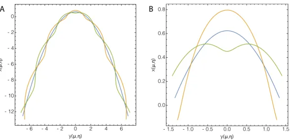
Figure 3. Superposition of the growing parabola and free holomorphic modes: on left in
green, k = 3,² = 0.12/cosh2(3), in orange, k = 3,² = −0.12/cosh2(3), in blue the non-perturbed parabolic shape. A tip-splitting event accompanies the side-branching on the curve in green but not on the orange-profile. So the undulated mode depends on the tip-perturbation. On the right: zoom on the tip.
which gives forη = 1 u = −sin(kµ) 4k2 {(4k 2 + 1) cosh(2k) − 3k sinh(2k) − 1} − µsinh(k)
2k cos(kµ)(2k cosh(k) − sinh(k))
v = −cos(kµ) 4k2 {(4k 2 + 1) sinh(2k) + k − 3k cosh(2k)} +sin(kµ) 2k {k(sinh 2(k) + cosh(k)2) − sinh(k)cosh(k)}. (29)
In Figure 3, we give several possible solutions for the new shapes at fixed wavenumber: k = 3 which means a wavelength close to the tip radius. At linear approximation, it is easy to obtain a tip-splitting event versus a dendrite but the two kinds of mode differ only at the tip which is a difference with viscous fingering. Concerning the shape of leaves, both undulating modes exist but the sharp tips seem to be the most common case. In the next section, we present another growth model triggered by diffusion: the poro-elastic model.
4. Nonlinear poro-elasticity in parabolic coordinates
Let us now extend the preceding analysis to the case of a simple nonlinear poro-elastic material. This model is well-suited to describe swelling gels but also, to some extent, the behavior of vegetal tissues as it incorporates both an elastic and a liquid phase. In response to pressure gradients, the liquid phase moves inside the solid phase in order to minimize the total energy of the system. At equilibrium, a nonlinear poro-elastic material is therefore equivalent to an elastic material with a space-dependent compressibility. As such it also provide a (highly simplifed) model of stress-modulated growth. Ignoring the mixing contributions arising from the interactions between the
solvent molecules and the polymer chains, the Helmoltz free energy is simply that of the highly compressible cross-linked polymer network [30]:
W =E 2(Tr(F
T
F − 2) − 2logdetF ) (30) so that the Grand potential to be minimized is simply:
E [~u] = E 2 Z ˜ V dµdη ( (∂ηx)2+ (∂ηy)2+ (∂µx)2+ (∂µy)2− 2h2µ (31) − 2 log à ∂µx∂ηy − ∂ηx∂µy h2 µ !) (32) −µ0 v Z ˜ V dµdη(∂µx∂ηy − ∂ηx∂µy − h2µ). (33) The first two terms in the equation above are just the Helmoltz free energy density integrated over the volume of the poro-elastic tip while the third integral enforces the molecular incom-pressibility constraint at the thermodynamic equilibrium. Hereµ0is the chemical potential of
solvent molecules in the particle reservoir in contact with the system and v is the volume per solvent molecule. In the context of plant sciences,µ0is sometimes referred to as the pore
pres-sure. Similarly to the growing case, we may obtain the Euler–Lagrange equations by requesting the Gâteaux derivative of the functionalE [~u] above to vanish and we obtain the following set of equations: J∆µ,ηx =∂log J ∂µ ∂y ∂η− ∂log J ∂η ∂y ∂µ J∆µ,ηy = −∂log J ∂µ ∂x ∂η+ ∂log J ∂η ∂y ∂µ (34) where: J =∂µx∂ηx − ∂ηx∂µy h2 µ . (35)
As previously suggested [31, 32], a swelling body is, at equilibrium, equivalent to a compress-ible structure subjected to an hydrostatic pressure at its free surface. This is illustrated by writing the boundary condition at the free surface in the following form:
STN =~ µ0 v JFF
−TN~ (36)
where the definition for the nominal stress has been kept:
S =∂W
∂F (37)
but now care must be taken to interpret S as the partial stress associated with the solid phase of the swelling material. Recalling that hµ=pη2+ µ2, it is not difficult to check that the following
solution: x = αηµ y =α 2(µ 2 − η2) and J = α2 (38) with α =q 1 1 −µ0 E v (39) is a nonlinear symmetric solution of the equilibrium equations and boundary conditions. This solution correspond to an homogeneous swelling process. The one-dimensional swelling ratioα is comprised between 0 and ∞ and is directly controlled by the dimensionless chemical potential
Martine Ben Amar and Julien Dervaux 623
of the solvent particles reservoirµ0/(E v). Let us now perturb the fields x, y, and J using the
following expansion: x = αηµ + ²αu(µ,η) y =α 2(µ 2 − η2) + ²αv(µ,η) J = α2+ ²α2j (µ,η). (40)
Inserting the expansions above in the equilibrium equations (34), we obtain the following equations: ∆u = − 1 α2 µ η∂j ∂µ+ µ ∂j ∂η ¶ (41) ∆v = − 1 α2 µ µ∂j ∂µ− η ∂j ∂η ¶ (42) where j is given by:
j = 1 η2+ µ2 ½ η µ ∂u ∂µ− ∂v ∂η ¶ + µ µ ∂u ∂η+ ∂v ∂µ ¶¾ . (43)
As previously, let us introduce the complex displacement U = u + I v and the complex coordi-natesζ = µ + Iη to obtain the following equations:
∆U = −2Iζ α2 ∂j ∂ζ (44) j = I ζ ∂U ∂ζ − I ζ ∂U ∂ζ. (45)
The previous equations can immediately be integrated to give, after using the symmetry condition with respect toµ:
U (ζ,ζ) =1 + 2α 2 2 + 2α2 ½F0 (ζ) 2ζ (ζ 2 − ζ2) + F (ζ) − F (ζ) ¾ (46) where F is an arbitrary holomorphic function with appropriate behavior at infinity (|u| < η|µ| and |v < |µ2− η2|) that must satisfy the linearized boundary condition (36):
∂U ∂ζ + ∂U ∂ζ + F 0 (ζ) = 0 for ζ = ζ − 2I (47) which cannot be satisfied for periodic holomorphic functions F , indicating that the swollen poro-elastic tip is also linearly stable.
5. Conclusion
Motivated by several discussions with Yves Couder, we have begun to investigate in this paper the behavior of growing elastic tips. By analogy with the shape of several biological structures but also with dendritic tips, we have chosen to describe growing tips as parabolas. We have derived the Euler–Lagrange equations ruling the shape of growing hyperelastic tips as well as nonlinear poro-elastic swelling tips, as a simple example of stress-modulated growth. In the case of homogeneous growth, as well as at the thermodynamic equilibrium for the swelling case, the parabolic tips were found to be linearly stable with respect to infinitesimal perturbations. Free harmonic modes, which may trigger a roughening transition depending on their dynamic and on the level of noise in the system, were also analyzed. More realistic models, incorporating additional constraints arising from boundary conditions and non-homogeneous growth will be considered in a forthcoming publication. Besides the problem of plant morphogenesis studied here, an understanding of the behavior of growing tips might also contribute to the design of
complex elastic structures using swelling gels [32, 33], inflatable structures [34] or electrically-actuated materials [35].
This work, suggested to both of us by Yves, is the outcome of our last conversations. We are convinced that he would have gently pushed us to explore more deeply the leading role of tips in biological growth processes.This is only a first contribution on his physical intuitions which have always combined universality and simplicity.
Conflicts of interest
The authors declare no competing financial interest.
Acknowledgements
MBA would like to thank the Isaac Newton Institute of Mathematical Sciences, Cambridge, for support and hospitality during the programe “Growth, Form and Self-Organization” where work on this paper was undertaken and also during the program “Complex analysis: techniques, applications and computations” where it was finalized. She also acknowledges the partial support from the Simons Foundation, the EPSRC grant no EP/K032208/1, the EPSRC grant no EP/R014604 and from ANR under the contract MECATISS (ANR-17-CE30-00007).
References
[1] Y. Couder, “Viscous fingering as an archetype for growth patterns”, in Perspectives in Fluid Dynamics (G. K. Batchelor, H. K. Moffatt, M. G. Worster, eds.), Cambridge University Press, Cambridge, 2000, p. 53-98.
[2] E. Lajeunesse, Y. Couder, “On the tip-splitting instability of viscous fingers”, J. Fluid Mech. 419 (2000), p. 125-149. [3] Y. Couder, O. Cardoso, D. Dupuy, P. Tavernier, W. Thom, “Dendritic growth in the Saffman–Taylor experiment”, Eur.
Phys. Lett. 2 (1986), p. 437-443.
[4] J. S. Langer, “Dendrites, viscous fingers and the theory of pattern formation”, Science 243 (1989), no. 4895, p. 1150-1156.
[5] M. Rabaud, Y. Couder, N. Gerard, “Dynamics and stability of anomalous Saffman–Taylor fingers”, Phys. Rev. A 37 (1988), no. 3, p. 935-947.
[6] M. B. Amar, P. Nassoy, L. LeGoff, “Physics of growing biological tissues, The complex cross talk between cell activity, growth and resistance”, Phil. Trans. R. Soc. Lond. A 377 (2019), 20180070.
[7] D. Ambrosi, M. B. Amar, C. Cyron, A. D. Simone, A. Goriely, J. Humphrey, E. Kuhl, “Growth and remodelling of living tissues: perspectives, challenges and opportunities”, J. R. Soc. Interface 16 (2019), no. 157, 20190233.
[8] S. Tanveer, “Surprises in viscous fingering”, J. Fluid Mech. 409 (2000), p. 273-308.
[9] E. A. Brener, V. I. Melnikov, “Pattern selection in two-dimensional dendritic growth”, Adv. Phys. 40 (1991), p. 53-97. [10] P. G. S. G. Taylor, “The penetration of a fluid into a porous medium or Hele-Shaw cell containing a more viscous
liquid”, Proc. R. Soc. Lond. A 245 (1958), p. 312.
[11] G. P. Ivantsov, “Temperature field around a spherical, cylindrical, and needle-shaped crystal, growing in a pre-cooled melt”, Dokl. Akad. Nauk SSSR 58 (1947), p. 567-569.
[12] B. Audoly, Y. Pomeau, Elasticity and Geometry, Oxford University Press, Oxford, 2010.
[13] R. W. Ogden, Non-linear Elastic Deformations, Dover Publications and Ellis Horwood Ltd., Chichester, 1984. [14] G. A. Holzapfel, Nonlinear Solid Mechanics a Continuum Approach for Engineering, John Wiley & Sons, Chichester,
2000.
[15] A. Goriely, The Mathematics and and Mechanics of Biological Growth, Springer-Verlag, New York, 2017. [16] G. Horvay, J. W. Cahn, “Dendritic and spheroidal growth”, Acta Metall. 9 (1961), p. 695-705.
[17] J. S. Langer, “Instabilities and pattern formation in crystal growth”, Rev. Mod. Phys. 52 (1980), no. 1, p. 1-28. [18] P. M. Morse, H. Feshbach, Methods of Theoretical Physics, McGraw-Hill, New York, 1953.
[19] M. A. Biot, “Surface instability of rubber in compression”, Appl. Sci. Res. A 12 (1963), p. 168.
[20] M. B. Amar, P. Ciarletta, “Swelling instability of surface-attached gels as a model of tissue growth under geometric constraints”, J. Mech. Phys. Solids 58 (2010), p. 935-954.
[21] A. L. Barabasi, H. E. Stanley, Fractal Concepts in Surface Growth, Cambridge University Press, Cambridge, UK, 1995. [22] J. Krug, “Origins of scale-invariance in growth processes”, Adv. Phys. 46 (1997), p. 139-282.
Martine Ben Amar and Julien Dervaux 625
[23] A. Cavagna, A. Cimarelli, I. Giardina, G. Parisi, R. Santagati, F. Stefanini, M. Viale, “Scale-free correlations in starling flocks”, Proc. Natl Acad. Sci. USA 107 (2010), p. 11865-11870.
[24] J. Dervaux, J. C. Magniez, A. Libchaber, “On growth and form of Bacillus subtilis biofilms”, Interface Focus 4 (2014), no. 6, 20130051.
[25] M. N. Barber, A. Barbieri, A. Angelo, J. Langer, “Dynamics of dendritic sidebranching in the two-dimensional symmetric model of solidification”, Phys. Rev. A 36 (1987), p. 3340-3349.
[26] M. B. Amar, V. Hakim, M. Mashaal, Y. Couder, “Self dilating viscous fingers in wedge-shaped Hele-shaw cells”, Phys.
Fluids A 3 (1991), no. 7, p. 1687-1690.
[27] Y. Couder, “Growth Patterns: From Stable Curved Fronts to Fractal Structures”, in Chaos, Order and Patterns (P. C. R. Artuso, G. Casati, eds.), Plemum Press, 1991, p. 203-227.
[28] S. Li, J. S. Lowengrub, J. Fontana, P. Palffy-Muhoray, “Control of viscous fingering patterns in a radial Hele-Shaw cell”,
Phys. Rev. Lett. 102 (2009), p. 1.
[29] M. B. Amar, “Anisotropic radial growth”, Euro. Phys. Lett. 16 (1991), no. 4, p. 367-372.
[30] W. Hong, X. Zhao, J. Zhou, Z. Suo, “A theory of coupled diffusion and large deformation in polymeric gels”, J. Mech.
Phys. Solids 56 (2008), p. 1779-1793.
[31] J. Dervaux, M. B. Amar, “Buckling condensation in constrained growth”, J. Mech. Phys. Solids 59 (2011), p. 538-560. [32] J. Dervaux, Y. Couder, M. A. Guedeau-Boudeville, M. B. Amar, “Shape transition in artificial tumors: from smooth
buckles to singular creases”, Phys. Rev. Lett. 107 (2011), 018103.
[33] E. Sultan, A. Boudaoud, “The buckling of a swollen thin gel layer bound to a compliant substrate”, J. Appl. Mech. 75 (2008), 051002.
[34] E. Siefert, E. Reyssat, J. Bico, B. Roman, “Bio-inspired pneumatic shape-morphing elastomers”, Nat. Mater. 18 (2019), p. 24.
[35] M. Pineirua, J. Bico, B. Roman, “Origami controlled by an electric field”, Soft Matter 6 (2010), p. 4491-4496.