QUARTERLY JOURNAL
OF ECONOMICS
Vol. LXXVII
August, 1963
No. 3
ECONOMIC GROWTH WITH TWO ENDOGENOUS FACTORS
JtiRG NIEHANS
Introduction, 349. — I. The two class model, 351. — II. The one class model: diminishing returns, 358. — III. The one class model: infinite growth with con-stant returns, 365.— Concluding remarks, 370.
INTRODUCTION
In Ricardian economics, growth was the result of the dynamic interaction between land, labor, and capital. Of this trinity, only land was exogenously given, whereas labor and capital were both determined endogenously. With the growing of doubts in the Mal-thusian theory of population, however, the main link in the causal chain leading from economic development to population became unserviceable. Since then, population and labor were mostly con-sidered as being determined by forces outside the economic system. This is particularly true in modern growth models. They usually
make capital the only endogenous factor of production while the supply of labor at each moment of time is assumed to be given. It is the purpose of this paper to establish a theoretical link between modern growth theory and the Ricardian tradition of treating labor as an endogenous factor.
To the statement that modern growth theory used to consider only one endogenous factor there is at least one notable exception. In his "Contribution to the Theory of Economic Growth" — and an important contribution it was — Solow also touched upon the con-sequences of introducing some Malthusian theory of population.1
1. Robert M. Solow, "A Contribution to the Theory of Economic Growth," this Journal, LXX (Feb. 1956) 90 ff. Stimulating hints can also be found in T. Haavelmo, A Study in the Theory of Economic Evolution (Amsterdam, North-Holland Publishing Co., 1954), pp. 39 ff. After this paper was finished my attention was drawn to the article by R. R. Nelson, "A Theory of the Low Level Equilibrium Trap," American Economic Review, XLVI (Dec. 1956), Pages 349-516 reprinted by Kraus Reprint Corporation.
His remarks, though very suggestive, were limited to one page, and he left it to his readers to follow up his hints. While the present paper was being worked out, its author did not remember the relevant page in Solow's article. When he was reminded of it, he found that, in fact, he seemed to have carried out just about what Solow had generously left to his readers.
This paper was written under the stimulating influence of a paper by Beckmann in which the assumption of a constant savings ratio was combined with a Malthusian population function.2 From the fact that these assumptions together with a production function
X = LaK0 imply infinite growth of population and capital even un-der diminishing returns to scale, Beckmann concluded that the pro-duction function had to be modified to bring the results more in line with reality. Despite the obviously finite character of the sur-face of the globe I could not quite bring myself to share Beckmann's concern about infinite growth, but at the same time the endogenous nature of labor in his model induced me to consider the problem in a more general way. Without Beckmann's paper, therefore, the present article would not have been written.
In the first part of this article the problem is discussed in terms of a two-class economy in which capital accumulation and propaga-tion result from different social classes. The second part analyzes the same question for the — probably more relevant — case of a one-class economy with particular reference to diminishing returns to scale. The final part concentrates on the special case of constant returns to scale, for which, of course, more definite results can be obtained.
The author is painfully aware of the shortcomings of his mathe-matical treatment of the problem. In many instances he is forced to rely on less than rigorous demonstrations of his points. He never-theless believes that these points can be established beyond reason-able doubt. For the rest, he is fully aware of the risk of being later contradicted by colleagues better equipped to solve systems of interdependent differential equations.
895 ff. Nelson's model, though using a different analytical technique, actually contains most of the basic elements of the model presented in the second part of this paper. I am sorry that I had overlooked it. The paper by Stephen Enke, "Population and Growth: A General Theorem," this Journal, LXXVII (Feb. 1963), 55 ff., appeared too late to be used in working out this article. It seems to indicate that in the present state of growth theory the ideas de-veloped hereafter really are "in the air" and thus, perhaps, not a very scarce commodity.
2. Martin Beckmann, "Wirtschaftliches Wachstum bei abnehmendem Skalenertrag," paper presented to the Theoretischer Ausschuss der Gesellschaft filr Wirtschafts- and Socialwissenschaften, February 1, 1963 (to be published).
I. THE Two CLASS MODEL
Let there be a production function with constant factor elastici-ties,
a
and 19, relating output (X) to labor (L) and capital (K):(1) X = LaKP (1 >
a > 0; 1
>P
>0).
Labor is assumed to be identical with total population for all prac-tical purposes. The obvious fact that not everybody belongs to the labor force is thus thought to be taken care of by the proper choice of units rather than by introducing some difference between population and labor force. Technical knowledge is assumed to be constant, and the problems of technical progress are not considered. Total population is thought to be divided in two classes. One of them propagates itself but does not save and can thus be called the "proletariat" in a literal sense. The capitalist class, on the other hand, is accumulating capital but produces no offspring be-yond reproduction.
The proportionate increase in population per unit of time is made to depend linearly on the difference between the actual wage rate and some minimum of subsistence wage, w., while the actual wage rate in turn is equal to the marginal productivity of labor:
,,, dL 1 L 3.X. tz)
dt Di.• L- . L- . p ( — — w.) .
Rostow would probably have identified p as some "marginal pro-pensity to proliferate." Malthusians will maintain that p is posi-tive. This is, in fact, the assumption on which this paper is based. It was often argued, it is true, that the rate of population increase varies in inverse proportion to real income, and the author of this paper does not claim expertise on the theory of population. He felt, however, it was best to concentrate on the Malthusian case because (1) in the light of modern population analysis it seemed to have somewhat more in its favor than the opposite case not only for underdeveloped countries but also for industrial societies, and (2) anyone holding the opposite view would find it easy to make the necessary modifications for himself. (These modifications would, of course, turn many conclusions upside down.) No matter how this question is decided, the population theory underlying these models is at best very crude. It seems to be still good enough, how-ever, — in part thanks to its very simplicity — to draw attention to certain important consequences of making population an en-dogenous factor.
352
QUARTERLY JOURNAL OF ECONOMICSof time may be made to depend on the difference between the
mar-ginal return of capital and some minimum return r„,:
dK 1
k( ar
k..i) — • — = — = s— — r
en).dt K K DK
s
is, of course, the marginal propensity to save out of profits. If
r„, = 0, it is equal to the average propensity to save or the savings
ratio. It is one of the distinctive features of the present analysis
that it allows for the possibility of some positive minimum return
on capital at which capitalists cease to save and begin to use up
their wealth. It will be seen that whether the economy tends to
infinite growth even with diminishing returns to scale or whether
its development leads to secular stagnation depends crucially on
the existence of such a minimum return.
Equations (1), (2) and (3) constitute the two class model. Its
basic characteristics are best analyzed in terms of a graph, in which
labor and capital are measured on logarithmic scales (cf. Figure I).
Figure I
The important elements of this graph are the (broken) lines of
equal wages or "iso-wage lines" and the (solid) lines of equal
capi-tal returns or "iso-return lines." They are all positively sloped
straight lines, their slopes being determined by the exponents of
the production function, a and P. For wages, the production func-tion yields
log w = log ( l
a
Z- ) = log a + (a — 1)log L + ft log K. ?ILWe now have to allow for variations in log L and log K in such a way that log w remains constant:
d(log w) = (a — 1) d(log L) + )3 d(log K) = 0, or
d (log K)
d (log L)
w = const
In the same way, the iso-return lines are described by the condition
d (log K)
d (log L)
a
1 — /3. r = const
If we move vertically upward in our graph we arrive at successively higher wage levels, for a given quantity of labor is combined with more and more capital. At the same time, capital returns are fall-ing, because for a given quantity of labor the marginal product of capital will fall if more capital is used. For similar reasons, if we move horizontally from left to right, capital returns are increas-ing while wages are fallincreas-ing.
At this point it is necessary to make specific assumptions about returns to scale. Let us start with diminishing returns. In this case a -I- /3 < 1. As a consequence, the iso-wage lines are sloping
— upward at an angle of more than 45 degrees, for 1
$
a
> 1. The iso-return lines, on the other hand, are rising at less than 45 de-grees, for--
a
13
--. < 1. This is the way Figure I is drawn.
We can now introduce the minimum levels of wages and capital returns. This is done by simply identifying the particular iso-wage line, wm, and the particular iso-return line, rm. If the two minimum
lines intersect in the first quadrant, they divide the graph into four sectors, characterized by different directions of the growth path (cf. Figure II). In the SW-sector, the quantity of both factors is increasing in the course of time, for both wages and capital returns
1 — a
are above their respective minimum. This is thus the area of un-equivocal growth. In the NE-sector the reverse is true, both factor prices being below their minimum. The economy is thus in full de-cline. In the NW-sector with its high wages and low capital returns, the labor force is growing, but capital is used up. At the same time the living standards of the working classes decline while the situa-tion of capitalists is improving. Finally in the SE-sector more and more capital is accumulated at falling returns, but population de-clines and real wages rise. Whenever the growth path is crossing the minimum wage line, its direction must be vertical, because popu-lation is constant. Conversely, if it crosses the line of minimum capital returns, it moves in a horizontal direction because capital is stationary. If by some accident the growth path should once reach the point where the two minimum lines intersect, it will stop there forever, because both factors then become stationary at the same time.
log K
log L
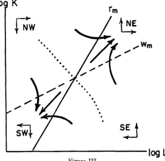
These considerations are far from being a perfect substitute for a solution of the system of underlying differential equations. I think, however, they are sufficient to draw certain general conclu-sions about the course of the growth path under diminishing re-turns to scale. The main point is that economic growth in this caselo• K
.
W
Wm
log L
Figure IIIgravitates toward the stationary state. The course of the path depends, of course, on the initial conditions. Some typical possi-bilities are indicated in the graph by (heavy) arrows. The path may approach its destiny of stagnation in quite roundabout ways, periods of capital accumulation being followed by periods of de-cumulation, periods of population growth by periods of population decline or vice versa. The over-all size of the economy in the final stationary state will be the bigger, the lower the two income minima. At the same time, however, a low minimum wage will lower the per capita income of the working classes, whereas a low minimum return on capital will make for low capital yields. There is thus a conflict between the size of the economy as a whole and the standard of living of its inhabitants.
As a limiting case it is possible to remove the stationary state ad infinitum by making either the minimum wage or the minimum capital return (or both) equal to zero. If population increases at any income, the economy will grow forever. The same is true if it saves at any income. The last mentioned case is actually the one which led Beckmann to the conclusion that even diminishing returns to scale would permit infinite growth. We now see that it is a limiting case and that inside of this limit Beckmann's conclu-sion does not hold. In general, Ricardo's stagnationist views seem to be vindicated.
We now turn to growth under increasing returns where
a + /3
> 1.
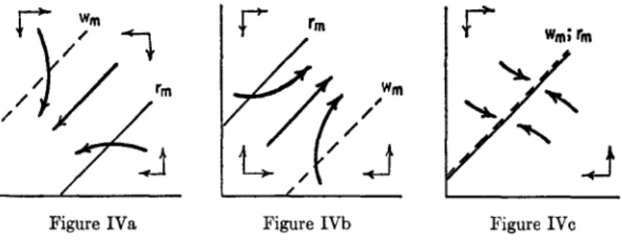
In this case it is the iso-wage lines which are sloping upward at less than 45 degrees, while the iso-return lines are now rising at an angle of more than 45 degrees. The resulting graph (Fig-ure III) thus resembles Fig(Fig-ure I with the important exception that the symbols for w1 • • • w,, and r1 • • • rg are interchanged. This change has far-reaching consequences for the growth path. The point where the two minimum lines intersect is still a point of secu-lar stagnation, to be sure, but it is now unstable. In the NE-sector, where both factor prices are above their respective minimum, the economy is moving away from the stationary state with increasing speed in a process of infinite growth with rising living standards. In the SW-sector, on the other hand, the economy is in a process of full decay with the vanishing point as its only limit. If the starting point is taken in the NW- or SE-sector, there will first be a phase of mixed growth and decline. This process will then take the economy to the threshold of one of the minimum lines, over which it enters the door to either eternal growth or eternal decline. Through the stationary point from NW to SE there must thus run a critical curve separating the starting points from which the econ-omy can take off for "self-sustaining growth" from those which damn it to eternal gloom. Those who believe in the "big push" will find good reasons for pushing an economy, which is still on the wrong side of the track, across the critical line into the take-off area.3There is finally the case of constant returns to scale with
a +
/3 = 1. It is characterized by iso-wage and iso-return lines all sloping upward at an angle of 45 degrees. The two minimum lines are thus parallel. As a consequence there is, in general, no stationary intersection point. The positions of the two minima are now all-important. If they are both relatively high, there will be no area in which both factors can grow at the same time, above-minimum wages requiring below-above-minimum capital returns and vice versa. Possibly after having passed through a period of transition, the economy will thus inevitably be sucked into the current of gen-eral decay (Figure IVa). If, on the other hand, both minima are relatively low, i.e., if the proletariat begins to proliferate and the capitalists begin to save at low incomes, then the economy will sooner or later move into an area where both factors increase. It is then in the stream of eternal growth (Figure IVb). There is, of3. That endogenous population growth may lead to "big push" arguments was already realized by Solow, op. cit., p. 91. His observation was later
amplified in a note by John Buttrick, "A Note on Professor Solow's Growth Model," this Journal, LXXII (Nov. 1958), 63 ff.
r
Wm; rmcourse, the borderline case, where the two lines coincide in the graph. (This does not mean that minimum wages and minimum returns are at the same absolute level, i.e., tv. = r,,,i; it just means that at those combinations of labor and capital, which result in minimum wages, capital returns are at their minimum too.) In this case, every point on the combined minimum line is a stable point of stationary equilibrium. From wherever it may be, the economy then approaches one of these stationary points where fur-ther development will come to an end (Figure IVc).
Figure IVa Figure IVb Figure IVc
This completes the discussion of the two class model. I believe it offers interesting insights into some possible mechanisms of dy-namic interaction of labor and capital. It is also relatively close to the Ricardian "vision" of the economy, and it is probably sus-ceptible of further mathematical analysis, particularly in the con-stant returns case. I doubt, however, if much further analysis of this model is actually warranted, because the two class assumption has some considerable drawbacks. There is, first, the problem of the "silent partner." Under diminishing returns to scale, not all income goes to labor and capital. The remainder may be imagined to go to the fixed factor, e.g., "land," which made the returns on labor and capital decline. Of these returns on "land," the two class model tacitly assumes that they influence neither capital accumula-tion nor propagaaccumula-tion, which seems to be a rather unsatisfactory assumption to make. The situation is hardly better in the constant and increasing returns cases where the "silent partner" receives zero or even negative incomes. Aside from this technical point, the assumption that there is a proletariat, living on wages only, which proliferates but does not accumulate, and a capitalist class, living on capital returns only, which accumulates but does not proliferate, does not seem to be a happy description of reality. This may, of course, be a matter of personal judgment, but I
can-not help feeling that the one class model offers more fruitful oppor-tunities for refinement.
II. THE ONE CLASS MODEL: DIMINISHING RETURNS
The one class model is again based on the production function (1). However, both capital accumulation and proliferation are now thought to be accounted for by the population as a whole, both depending simply on real income per capita
X
Y =
L.
There is again a certain Malthusian subsistence level of per capita income, mL, above which population is increasing, while at lower levels it will decline. The increase in the labor force (or popula-tion) per unit of time thus becomes
dL •
(4) —
dt = L = p(y — mL) L,
where p now ,measures the sensitivity with which population reacts to differences between actual income and subsistence income. For the rest, the remarks on the population function in the two class model mutatis mutandis apply here, too.
Similarly, per capita capital accumulation is assumed to depend linearly on the difference between actual per capita income and some critical level, mK. For total capital formation per time period this yields
dK fr.
(5) — = n. = 8(y — mK)L. dt
This is nothing but an old-fashioned Keynesian savings function,
s being the marginal propensity to save. It should be noted that the subsistence minimum with respect to population, mL, will in general be different from the subsistence minimum with respect to capital, mg. Indeed, it will appear that the relative position of the two minima may be of critical significance for the long-term growth prospects of an economy.
On the basis of this model we again want to know what course the growth path will follow from any given point of departure. This depends, among other things, on returns to scale. In this sec-tion the discussion will concentrate on the case of diminishing re-turns. Analysis of the constant returns case will be postponed to the following section, while the less relevant case of increasing re-turns is not explicitly considered.
K
First we have to determine the shape and direction of the lines of equal per capita income or iso-income lines. It is easily seen that on logarithmic scales they appear as straight lines, their slope being determined by the exponents of the production function. For log y we obtain
X
log y = log —
L = log (La-1/0) = (a— 1) logL /3logK.
In order to keep income constant, we have to keep its logarithm constant:
d(logy) (a — 1) d(log L) d(log K) = 0.
It follows that iso-income lines must satisfy the requirement
d (log
K)
1 — a(6) —
d (log L)
Along each line, the elasticity of capital with respect to labor is constant. Under diminishing returns to scale, i.e., with a + # < 1, this expression is greater than unity. The iso-income lines are thus parallel straight lines sloping upward at an angle of more than 45 degrees. For what follows, it is more convenient, however, to think in terms of natural scales. The iso-income curves are then curving upward from the origin (Figure V). This means that in order to keep per capita income constant, more and more capital has to be
added if labor increases by equal amounts. Income increases, of course, as we move upward and to the left, for a given amount of labor is then combined with more capital.
In the resulting spectrum of iso-income curves we now have to identify the two subsistence levels. Three cases may be distin-guished according to whether mg. We shall first focus atten-attention on the case where mz, > mx, so that there is a certain range of incomes in which people save but do not maintain their numbers. This case is illustrated in Figure V. On the basis of this graph it is easy now to determine the general direction of the growth path. Below mx both factors will decline. As a consequence, the growth path is heading downward and to the left. Between the two mini-mum lines, the stock of capital is increasing, but population still declines. If income is above the population minimum, too, both factors will be growing and the economy is heading upward and to the right. Whenever the economy crosses the ms-line, its growth path, capital being stationary, is horizontal, while on the mL-line, where population is stationary, it is vertical. This can be checked mathematically by inspecting the sign of the quotient of (4) and
(5) :
(7)
s
yL
p y— mLOne additional bit of information on the growth path is ob-tained by analyzing its curvature. From (7) we obtain
(8) d(
K)
s —(— =
• dy.
L p (y — mL)2
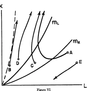
If mL > mx, this expression is negative for positive dy. This means that with increasing per capita income, the growth path is curved clockwise, while with falling income it is curved counterclockwise. It is now possible to trace the main outlines of the growth path (Figure VI) . Starting from a point below — but not "too far" below — the capital minimum (A), the economy will first go through a phase of shrinking capital and population, while at the same time per capita incomes increase. Sooner or later, this will bring it to the n4-fine where capital accumulation sets in. In the course of 4. Choosing plausible values of the parameters and various starting points, Dr. D. Onigkeit computed several different growth paths. The result reproduced every significant aspect of the free-hand curves of Figure VI and was thus in agreement with the mathematical considerations given below. The computing facilities were kindly made available by the Computing Center of the University of Zfirich.
L
Figure VI
time, the continued increase in living standards will carry the
econ-omy across the m
L-line, too. From then on, both capital and labor
will be growing. For a while, the standard of living will continue
to increase, but even in the absence of a rigorous mathematical proof
we may strongly suspect that sooner or later it will reach a
maxi-mum. This can best be seen by considering a limiting case. Let
us assume
m
r, and m
gare rather close together. By selecting our
point of departure on a curve of very high income (B), we can then
bring (y — m
x)/ (y — m
r) in (7) close to unity. The growth path
thus becomes practically linear, its slope being determined by
s/p.If at our point of departure, per capita income is falling rightaway,
there is no problem. If, however, it first happens to rise, we must
sooner or later reach a point where it just touches one of the
upward-curving iso-income lines. At this point, per capita income has
reached its maximum. It is true that in general the growth path
will not be exactly linear, but this works in favor of the argument,
for as long as incomes are rising, the growth path is curved
clock-wise, whereas the iso-income curves are sloping upward
counter-clockwise. The point of tangency will thus be reached all the sooner.
It can also be said that within any finite time range the growth
path cannot follow the same iso-income line for more than just a
moment, for the iso-income lines are curved upward, while the
362 QUARTERLY JOURNAL OF ECONOMICS
growth path, if income is constant, is linear (cf. equation 8). As a consequence, per capita income cannot remain constant in the course of economic development. It cannot, therefore, stay at its maximum. The moment it ceases to rise, it must begin to fall. From then on, the growth path will be curved counterclockwise. The continuing decline will bring per capita income back closer and closer to the mL-line without ever crossing it and without even completely reaching it within any finite time span. However, if we could follow the growth path into an infinitely distant future, we would indeed see it proceed along the my-line. Graphically, the direction of the my-line would then be vertical, and we know that on the my-line the direction of the growth path is vertical, too. Alge-braically, (6) gives the slope of an iso-income line as
dK 1 — a K
dL = i3 L '
Since, by (1) together with the definition of per capita income y = X—, we have
L
1-a 1
K = L P . i,
this could be written as
dK 1 — a 1-a-13 1
= - L fi • 713.
dL p
If the growth path is to proceed along an iso-income line, this ex-pression must equal the slope of the growth path represented by
(7) :
1— a 1-a-s 1 8 y
— ms
L 13 • 1113 — :
p
P Y — mr,If L approaches infinity, y must thus approach either mL or zero.
The population minimum my will be approached as we let the
econ-omy grow into an infinite future, while the zero level will be ap-proached if we follow the growth path back toward the beginning of time.
Indeed, the eventual fall in per capita income is far from stop-ping over-all economic growth. In fact, capital and population will never cease to grow, diminishing returns notwithstanding. This follows from the simple fact that the growth path cannot cross the population minimum from above, since in this area it must move vertically upward. Just imagine that by some accident the con-tinuous fall in per capita income would bring the economy back to the population minimum. Population growth would then stop, but
capital would still be accumulated. As a consequence, per capita income would rise again, and the economy would be back in the growth area. Once the economy has stepped across the popula-tion threshold into the realm of growth of both factors, the door is closed behind it. Even if we followed it into an infinite future it would still expand along the mL-line. There is no need explicitly to consider the course of economic development from starting points above the capital minimum mx (e.g., C and
D),
because the fore-going paragraphs contain all that is necessary in the context. There is, however, a special case which requires attention. It seems very likely that there is an area of very low income, where the initial decline in capital and population will not improve living standards but rather depress them still further(E).
From such a starting point, the economy will never be able to reach the area of self-sustaining growth but will forever remain in a state of decay. Again one feels tempted to call for a "big push." This danger area will be the smaller, the lower the income, mr, at which people begin to save, and if saving is a constant fraction of income, i.e., mx = 0, it disappears completely. A low saving threshold thus seems to be something like an insurance against permanent decay.Let us now change our previous assumptions and concentrate
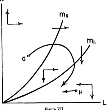
K
on the case mL < mk (Figure VII). Above the higher and below the lower minimum, the general direction of the growth path will be the same as before. Between the two minima, however, it will now be reversed, population increasing while capital is used up. The previous statements about curvature must be reversed too, for with increasing per capita income the slope of the growth path will now increase while with falling income it will turn around clock-wise, i.e., equation (8) is now positive for positive income changes. Starting from a point above the capital minimum (G) , the growth path will thus pass gradually from vigorous growth to eternal decay. If the economy starts somewhere in the area of decay (H), instead of in the growth area, it has no chance ever to get out of it under its own steam. Not even a "big push" can help much, because the economy would soon slip back into decay. It thus appears that the relative positions of the population minimum and the capital mini-mum can be of crucial importance for the long-range growth pros-pects of the economy, the chances for self-sustaining growth being the better and the risk of doom being the smaller, the higher the population minimum in relation to the capital minimum.
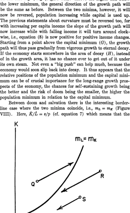
Between doom and salvation there is the interesting border-line case where the two minima coincide, i.e., ?ft = mK (Figure VIII). Here, It/L = s/p (cf. equation 7) which means that the
K
L
growth path becomes a straight line with positive slope moving
upward and to the right above the combined minima (Q) and
down-ward and to the left below
(R) .There will now be a definite limit
to expansion and decay, for every point on the minimum line now
is a point of stationary equilibrium. From above as well as from
below the economy will thus be heading straight — but with
dimin-ishing speed — toward secular stagnation somewhere on the
mini-mum line. Again there is likely to be an area of perpetual decline,
though, from which even the stationary state cannot be reached
(S).
This completes the discussion of the case of diminishing
re-turns to scale. It showed that even with a fixed factor, say "land,"
a wide variety of growth patterns, ranging from infinite growth to
perpetual decay, is possible depending on the starting point, the
marginal propensities to save and to proliferate and, above all, the
incomes at which people begin to save and population begins to
grow. There is thus a remarkable difference between the
implica-tions of the one class and of the two class model. However, the
most desirable pattern, i.e., eternal growth combined with a
con-tinuous improvement of living standards, seems to be unattainable
under diminishing returns. As in the case of the two cg,ss model,
these results could not be established rigorously, because the
under-lying system of interdependent differential equations proved to be
quite intractable within the range of mathematical tools available
to the author. Part of this gap will be filled in the final section for
the much simpler case of constant returns.
III. THE ONE CLASS MODEL: INFINITE GROWTH WITH CONSTANT RETURNS
In itself, the special case of constant returns
(a -I-13 = 1)may
not be very important, for it would be curious indeed if in the real
world returns to scale were ever exactly constant. Its great
sig-nificance rather arises from the fact that it permits many results
to be established in a relatively simple way which for variable
re-turns, though we may believe them to be largely true, can at best be
established with considerable difficulty. It is with constant returns
models as with many other models: they are interesting exactly
because of their hoped-for relevance for such cases in which their
assumptions do not strictly apply. In particular, with the help of
the constant returns assumption it will be possible to give definite
answers to questions like those about the significance of the
pro-QUARTERLY JOURNAL OF ECONOMICS
pensities to save and to proliferate and of the two income minima on long-range per capita income and the growth rate.
The discussion will be limited to the case in which mL > so that, except for some special cases, the economy will eventually grow without limit. Also we will concentrate on the actual growth area while the area of decay, important though it may be, will not be further considered. In symbolic language this means that y> mL.
We may first raise the question whether there is now some iso-income curve, defined by the "equilibrium income" 9, which the growth path would follow forever once it were put on it. Such an equilibrium income indeed exists. This can be seen as follows. We know from equation (8) that the growth path becomes a straight line whenever per capita income is constant (i.e., dy = 0). On the other hand, we know from equation (6) that with constant returns to scale the iso-income lines are straight lines. It follows that if at any point the growth path has the same slope as the iso-income line going through that same point, it will run along this iso-income line forever after. Thus all we have to do is to determine that per capita income level at which the growth path has the same slope as the iso-income line. Under constant returns, iso-income lines are defined by the condition
dK K —= yi-a1 dL L
while the slope of the growth path is given by
dK s (y— ms)
=
dL p (y — mL)As the condition for the growth path following an iso-income line we thus obtain
1 8 (51 MK)
(9) —
P (51 — mL)
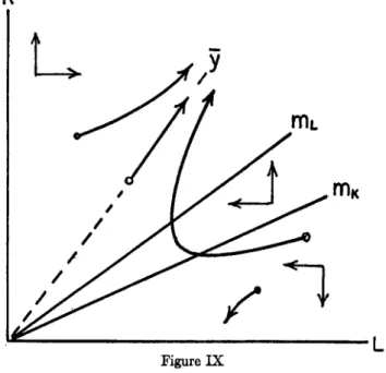
It is seen that the equilibrium income level only depends on the parameters a, 8, p, mL, and ms. From whatever point we start, the equilibrium income is thus the same. Once some growth path has reached 51 as determined by equation (9), per capita income will thenceforth remain constant. Within the assumptions of this sec-tion (mr, > ms; y > mL) there will be just one such income level, for the slope of the growth path given by the right-hand side of equation (9) will start with infinity at y = mr, and with increasing y will fall monotonically1towards s/p, while the slope of the iso-income lines given by y1-a will start at m2-a and rise with
in-creasing y. As long as income is below 9, the growth path is
cross-ing successively higher income levels, but wherever income is above
9, the growth path crosses the iso-income lines from above to go to
lower per capita levels. We may thus strongly suspect that from
both sides the growth path is moving asymptotically toward the
equilibrium income level. This is depicted in Figure IX.
K
Figure IX
We conclude that under constant returns to scale the economy will
in the long run follow a balanced growth path with constant per
capita income, unless it starts in some very low income area of
cumulative decay.
5Our next task will be to determine how equilibrium income 9
reacts to changes in the marginal propensities to save and to
pro-liferate and in the two income minima. These questions can be
an-swered by determining from equation (9) the sign of the derivatives
of 9 with respect to
s,p,
?ft,and m
g.
For the marginal propensity to save this derivative is
d9 _
1ds 1_7,1 ( 1 1 5, — mr, mi, — ins ).
PY
+
\ 1 — a 5/ 5/ — MK — mK)21
5. There is actually another equilibrium income below ma. It is un-stable in the sense that at the slightest disturbance the growth path is moving away from it either into sustained growth or into decay.
Within our assumptions, this expression must be positive. We con-clude that equilibrium income is the higher, the higher the propensity to save. For the marginal propensity to proliferate we obtain
d5, 1
dp 1
). (____
1
1
5
,—
mirmr, —
mir )85)4-1 1—a5? 9 — ML
+
(9 — 9702which must be negative. Equilibrium income will thus profit from any reduction in the sensitivity of population growth to changes in income. In the same way, the influence of the population subsistence minimum mi, is determined as
d51
_7 = •
UML ML - mil- 1 5, — mi,
+
5, — mK 1 —a 51Since this is positive, it follows that the standard of living will in the end be the higher, the higher the income level at which popula-tion begins to increase. The reverse is true for the minimum level of capital accumulation, for
d5,
=
1dmK mr, — mK
+
1 9 — Mg9 — ML 1 — a 9
must be negative. Per capita income will thus go the higher, the lower the income at which people begin to save. These results all agree well with intuitive expectation.
This leaves the more interesting question of the growth rate. We know that in balanced growth with constant returns to scale
L k
k
— = — = -- = g
L K X
We are thus free to judge the growth rate either on the basis of labor, of capital, or of production. In the present context it seems most convenient to use labor. From (4) we know that
L
_
g= 7: =P(Y —
mL),where 5, is itself a function of s, p, mL, and mK. So all we have to do is to take the derivatives of g with respect to each of these para-meters. Starting again with the propensity to save,
dg d5,
which must be positive, since
d9/ds
is positive. The rate of bal-anced growth will thus increase with an increase in the propensity to save. The proposition established by Solow that the propensity to save has no lasting effect on the growth rate thus seems to be in-valid in a world in which labor is endogenous.6 In such a world, the propensity to save indeed appears to be of quite decisive im-portance for long-term growth. This conclusion agrees well with common sense, for if a high rate of capital accumulation also en-courages the growth of population, it would be rather surprising if it had no effect on the long-term growth of both factors.For the effect on the growth rate of the marginal propensity to proliferate we obtain
dg
d9
c
iii,= (5! — ?ft) +
P—
dp.
Since
d9/dp <
0, this expression can be positive or negative. Whereas the effect of p on equilibrium income is unambiguously negative, its effect on the rate of growth thus seems to be ambiguous, depending on the other parameters. This is basically because popu-lation growth on the one hand encourages the growth of production, while on the other hand it lowers per capita income and thus dis-courages capital accumulation and helps to slow down the growth of production.The reaction of the growth rate to an increase in the popula-tion minimum mr, can be judged from
dg
= p( d9 — 1).
dm
Ldmi,
The sign of the expression in brackets is again ambiguous. By elementary operations it can be shown to depend on the sign of (4—mK). Without knowing more about the parameters it is there-fore impossible to say whether a high population subsistence level is good or bad for the long-range growth rate.
For the effect of the capital accumulation minimum, however, we obtain a definite result, for
dg
= pd9
dMK dmx
must be negative. The lower the income at which people begin to save, the faster will be the growth process in the long run.
6. This conclusion is already implied in Solow's remarks on variable population growth (op. cit., p. 90).
CONCLITDING REMARKS
This is about what I am able to say at the present time about economic growth with two endogenous factors. I am far from be-lieving that the simple models on which the analysis was based could be used to predict the actual course of economic history by simply estimating the parameters. Too many important factors were left out of account completely, technical progress being one of the most notable among them. Also the basic assumptions about capital accumulation and population were conspicuous more for their sim-plicity than for their close accordance with the results of modern research in these fields. I hope, however, that this paper was able to accomplish three things, viz.:
(1) to draw attention to some important interactions between capital formation and (endogenous) population in the process of economic growth,
(2) to present a simple technique with the help of which at least the first steps in the analysis of these interactions can be taken, (3) to submit a series of substantive propositions about the effects of population and savings behavior on the growth process. In particular, it was shown that in the two class model, except for certain limiting cases, diminishing returns set a finite limit to economic growth, whereas in the one class model they do not neces-sarily prevent economic growth from going on forever. It was also shown. that in a one class world the relative position of the in-come levels at which people begin to save and to increase their num-bers can be of about the same crucial importance for the course of growth as returns to scale in the two class model. For the special case of constant returns it was finally determined how the various savings and population parameters affect long-term income and growth.
The process of growth was also seen to depend on the starting point. Its most remarkable twists and turns were indeed found relatively near to this point, while in the course of time it tended to assume a more monotonic behavior. One might perhaps be tempted to argue that the "real" origin of an economy usually lies in the indefinite past, so that, in fact, the relevant part of any growth path is the one close to "infinity," while the dynamics of the "starting period" are of interest mainly for the historian. This argument would be valid if the relevant parameters had remained constant throughout history. In fact, however, these parameters will hardly ever remain the same for a very long time. Whenever they change,
we are at a new "starting noint." The more often they change, the more relevant thus becomes the area in the neighborhood of the starting point while the indefinite future is losing its interest. In the light of this consideration I feel that the analysis of this paper should be applied not so much to the growth prospects of an econ-omy in the very long run as to the dynamics of its development in the period soon after a given change in population and savings be-havior has occurred.