Discovering new languages from the study of games semantics

HAL Id: hal-00413040

https://hal.archives-ouvertes.fr/hal-00413040

Preprint submitted on 3 Mar 2010

HAL is a multi-disciplinary open access

archive for the deposit and dissemination of sci-entific research documents, whether they are pub-lished or not. The documents may come from teaching and research institutions in France or

L’archive ouverte pluridisciplinaire HAL, est destinée au dépôt et à la diffusion de documents scientifiques de niveau recherche, publiés ou non, émanant des établissements d’enseignement et de recherche français ou étrangers, des laboratoires

Discovering new languages from the study of games

semantics

Alexis Goyet

To cite this version:

Discovering new languages from the study of games

semantics

Alexis GOYET

under the supervision of Russ Harmer (PPS) and Pierre Louis Curien (PPS) 23rd of August, 2009

In compliance with the rules set by the MPRI (Master Parisien de Recherche en Informatique1), this master thesis starts with a 4 pages sum-mary in French, followed by a 2 pages “syntetic overview”. The main body of the thesis starts on page 7.

Summary

La s´emantique des jeux fut cr´e´ee pour donner un mod`ele du langage PCF ([2] et [3]). Cette d´emarche a ´et´e adapt´ee depuis `a d’autres cas, partant d’autres langages et cherchant `a les munir de nouvelles s´emantiques.

La motivation de notre approche est diff´erente : nous nous int´eressons `

a un objet s´emantique pr´eexistant - l’ensemble des strat´egies cellulaires, d´ecrite par Russ Harmer dans [4] - et cherchons son interpr´etation en termes de langages. Parce que cet objet n’est pas en relation directe avec l’ensem-ble des strat´egies innocentes, qui correspondent `a la s´emantique de PCF, le langage obtenu est enti`erement nouveau.

Nous donnons en fait deux langages pour ces strat´egies cellulaires : une syntaxe sp´ecifique, qui provient d’une premi`ere approche directe ; et une syntaxe g´en´erique, obtenue comme cons´equence d’une d´emarche de g´en´eralisation men´ee sur la s´emantique des jeux. Cette g´en´eralisation va au del`a de son but initial ; elle introduit des notions g´en´erales d’enregistrements et d’op´erateurs `a historique sur les jeux. Ceci rend la syntaxe g´en´erale com-mune `a un vaste ensemble de classes de strat´egies (y compris les strat´egies in-nocentes et cellulaires), tout en rendant visibles, sur les termes, une sym´etrie nouvelle entre fonctions et environnements.

1

La syntaxe sp´ecifique

Seule une pr´esentation informelle de cette syntaxe est donn´ee (y compris dans le rapport). Le but est uniquement la comparaison avec la syntaxe g´en´erique, qui constitue un meilleur cadre pour donner formellement un language pour les strat´egies cellulaires. La syntaxe est la suivante :

t::=| x | Ω

| recordr1...rm(λx1. . . xn.t)

| recordr1...rm((t)t1. . . tn)

| ϕ(r)t1. . . tn

O`u x, x1. . . xnsont des noms de variables, r, r1. . . rndes noms d’enregistrements2, et ϕ est un nom de test.

Lorsque recordr(s′) apparaˆıt comme sous-terme d’un terme s1, cela cor-respond `a la requˆete, de la part de s1, que la premi`ere ´etape de l’ex´ecution3 de s′

soit ”enregistr´ee” dans r. Lors de l’interaction de s1avec un autre terme s2, au moment de l’ex´ecution de s′, un objet r est cr´e´e pour r´epondre `a cette requˆete. Cet enregistrement r est cr´e´e en tant qu’objet de s1; diff´erentes copies de sous-termes de s1 peuvent alors y acc´eder, incr´ementant l’enreg-istrement. Le terme s1 peut ensuite faire un branchement conditionnel en fonction de la valeur de l’enregistrement r, avec un sous-terme de la forme ϕ(r)t1. . . tn(le prochain terme ex´ecut´e d´epend de la valeur de r et du test ϕ).

Un terme de cette syntaxe sp´ecifique peut donc avoir acc`es `a plus d’infor-mation qu’un terme de PCF, grˆace aux enregistrements. Ceci correspond `a une modification de la condition de d´ependance (la somme des informations dont les actions d’un terme peuvent d´ependre).

Mais, pour correspondre aux strat´egies cellulaires, la condition de

vis-ibilit´e (sp´ecifiant les actions que le terme peut effectuer) doit ´egalement ˆetre modifi´ee. Cette fois, il suffit d’appliquer une restriction par rapport `a PCF, qui s’effectue simplement au niveau du typage. Ce typage utilise une structure de pile pour l’environnement ; appeler une variable li´ee peut ainsi d´epiler, et donc perdre, l’acc`es `a d’autres variables.

La syntaxe g´en´erique

Dans le λ-calcul habituel, les noms de variables repr´esentent des fonctions que le terme peut appeler ; nous les appelons donc des noms de fonctions.

2

Nous n’utiliserons pas le terme d’”enregistement” en son sens habituel, ce qui de-vrait ´eviter toute confusion. Cette ambigu¨ıt´e n’est pas pr´esente en anglais, o`u le terme ”recording” (et non ”record”) est utilis´e.

3

Au cours d’une β-r´eduction avec une strat´egie lin´eaire de tˆete, la r´eduction se fait suiv-ant un certain ordre sur les sous-termes, qui correspond `a l’ordre des coups en s´emantique des jeux.

La syntaxe g´en´erique introduit, sym´etriquement, des noms d’arguments :

t::=| x | Ω | λx1. . . xn.t | tu1...un

(v1 : t) . . . (vm: t)

O`u les x1. . . xnsont des noms de fonctions, et les u1. . . un, v1. . . vm sont des noms d’arguments.

Si le terme f attend n arguments, la construction fu1...un

leur associe les noms d’arguments u1. . . un. Pour passer un argument a`a f , il faut ensuite utiliser (ui : a), ce qui pr´ecise quel argument est transmis. Cette pr´ecision serait superflue dans PCF, puisque l’ordre de passage des arguments suffit `a lever toute ambigu¨ıt´e. Mais ici, l’application est plus g´en´erale : il est possible de ”passer” au terme t l’expression (vj : t), o`u vj n’est pas l’un des ui. Le nom vj d´esigne alors l’un des arguments demand´e auparavant, lors d’un autre appel de fonction de la forme gv1...vm)

. Le nom d’argument vj est le sym´etrique du nom de fonction que g a attribu´e `a cet argument (disons x). Lors de sa premi`ere action, f peut appeler x ; dans ce cas, c’est le terme t qui sera pass´e comme valeur pour x, ind´ependamment de toute autre occurrence (vj : t′) (notamment si une autre valeur a d´ej`a ´et´e pass´ee pour x). Une description formelle de la r´eduction est donn´ee dans le rapport.

Lors de la β-r´eduction usuelle d’un terme de PCF, le deuxi`eme appel d’une variable x brise une certaine sym´etrie entre fonction et environnement. La valeur initiale de x est dupliqu´ee, et pass´ee `a nouveau. Cette valeur peut ˆetre vue comme une continuation ; la dupliquer force donc l’environnement `

a revenir sur ses pas, lui faisant perdre la m´emoire de l’interaction qui s’est d´eroul´ee depuis le premier passage de la valeur de x. La possibilit´e pour l’environnement de nommer aussi x r´etablie cette sym´etrie.

La d´emarche s´emantique

Dans la s´emantique des jeux, l’interaction entre une fonction et son en-vironnement est repr´esent´ee par une partie entre deux joueurs, dans un jeu dont les r`egles sont d´etermin´ees par les types. Lorsqu’une fonction est appel´ee, elle doit indiquer la valeur de son r´esultat, ce qu’elle peut faire en appelant une fonction de l’environnement ; la main est alors pass´ee au second joueur (repr´esentant l’environnement). Les fonctions sont ainsi des strat´egies sur le jeu.

La pr´esentation usuelle d´efinit un ´etat du jeu comme l’historique complet de l’interaction pass´ee. Chaque nouveau coup doit indiquer un coup qui le

condition autoriserait des comportements ne correspondant `a aucun terme de PCF ; ces termes correspondent en fait `a l’ensemble des strat´egies v´erifiant ´egalement la condition d’innocence. L’innocence restreint la ”vue” qu’une strat´egie a de l’historique de l’ex´ecution. La vue est une sous s´equence de l’historique, correspondant exactement `a la branche du terme qui a d´ej`a ´et´e ex´ecut´ee. Il s’agit des seules informations dont dispose la strat´egie pour choisir son prochain coup (condition de d´ependance), et, en mˆeme temps, des seuls coups disponibles pour justifier le suivant (condition de visibilit´e). Ainsi, l’appel d’une variable, qui est justifi´e par le coup correspondant `a son abstraction, doit apparaˆıtre dans la branche du terme d´ej`a ex´ecut´ee (c’est-`a-dire dans la vue).

Dans le cas des strat´egies cellulaires, les conditions de d´ependance et de visibilit´e utilisent des notions de vue dont l’une est plus permissive, et l’autre plus restrictive que la vue des strat´egies innocentes. Il s’agit donc d’un type de contrˆole d’acc`es plus fin, impos´e aux strat´egies.

La syntaxe g´en´erique permet de voir ces deux diff´erents types de contrˆoles d’acc`es simplement comme des conditions statiques sur les termes (c’est-` a-dire des m´ethode de typage). Le point le plus frappant est que, pour les strat´egies cellulaires, la condition de visibilit´e (qui fait appel `a la notion, peu naturelle, d’enregistrement) correspond `a appliquer aux noms d’argu-ments la condition de visibilit´e donn´ee pour les noms de fonctions dans la syntaxe sp´ecifique (typage avec pile). La syntaxe g´en´erique exhibe cette r´egularit´e nouvelle car elle est le produit d’une d´emarche de g´en´eralisation men´ee sur la pr´esentation de la s´emantique des jeux.

Cette g´en´eralisation ´etait initialement motiv´ee par la recherche d’une structure cat´egorique riche sur les strat´egies cellulaires, comme celle pr´esent´ee dans [5] par Harmer, Hyland et Melli`es, pour les strat´egies innocentes. Dans [5], la condition d’innocence correspond `a un foncteur, et la composition des strat´egies est rendue possible par des propri´et´es de ce foncteur.

Notre g´en´eralisation permet d’obtenir l’´equivalent de ce foncteur pour la notion de cellularit´e ; ceci permet de voir que les strat´egies cellulaires n’ont malheureusement pas de structure ´equivalente `a celle montr´ee dans [5]. N´eanmoins, la g´en´eralisation fait apparaˆıtre une condition plus faible, qui est suffisante pour d´ecrire la composition. Il s’agit de la notion d’op´erateur

`

a historique, qui englobe l’innocence et la cellularit´e. Cette approche se base sur des d´efinitions plus g´en´erales pour les jeux eux-mˆemes, faisant ´egalement apparaˆıtre une notion de plongement entre jeux.

Cette notion de plongement, qui caract´erise de mani`ere locale un rapport entre deux jeux, est un concept central dans notre d´emarche. Il constitue en premier lieu un outil essentiel dans les preuves ; les op´erateurs `a his-torique garantissent par exemple un certain nombre de plongements. Mais un plongement est ´egalement, en lui-mˆeme, l’expression d’un certain contrˆole

d’acc`es : un plongement de A dans B envoie toute strat´egie de A vers une strat´egie de B dont les actions, mais aussi les informations, sont restreintes. La syntaxe g´en´erique donne alors un terme pour chaque strat´egie de l’op´erateur `a historique maximal $, dans lequel plongent tous les autres ; la correspondance est exacte. Grace `a ces mˆemes plongements, ce langage est commun `a tous les op´erateurs `a historique, et en particulier aux strat´egies cellulaires. Mieux, chaque op´erateur `a historique correspond `a une condition statique sur les termes. Tous ces termes peuvent donc interagir `a travers la β-r´eduction de la syntaxe g´en´erique.

Synthetic overview (”Fiche synth´

etique”)

Game semantics was first presented in [2] by Hyland and Ong (and inde-pendently in [3], with another presentation), to give a fully abstract model of PCF. Each step of the (head linear) β-reduction corresponds to a move in a game ; different terms of the same type corresponding to strategies on the same game.

In the original presentation, the state of the game is defined as the full history of the interaction up to the current point (along with additional informations). With this definition, not all strategies correspond to PCF terms ; the model is given by the innocent strategies. Innocence is a condition which restricts the part of the history which may be used by the strategy. This subsequence of the history is called P-view (player view) ; it corresponds exactly to the branch of the PCF term already executed.

Other kinds of views have been defined, to give models of other languages in the same hierarchy as PCF. For example, enforcing no condition corre-sponds to the λ-calculus with (arbitrary type) references, which contains PCF.

The problem studied

The initial problem was the study of a set of strategies, called cellular, recently described by Russ Harmer in [4], which is yet unpublished. Con-trarily to innocence, cellularity uses two different kind of views for visibility (which actions can be performed) and dependency (what information is avail-able). The motivation was to strengthen the visibility condition of innocent strategies (through a translation) ; but the translated strategies broke the dependency condition, which had to be weakened.

The resulting condition is thus neither stronger, nor weaker than inno-cence. For example, a cellular function can count the number of times it has been called, which an innocent function cannot. Even more unusual is the fact that this object comes purely from the study of the semantics (cellular strategies, with the initial definition, play a central role in proofs of decid-ability of contextual equivalences) : it did not correspond to any language. Finding such a language was thus the first task of this internship.

The proposed contribution

We first obtained a specific syntax for cellular strategies. We then aimed to study the categorical structure of these strategies, by adapting recent work of Harmer, Hyland and Mellies ([5]), in which innocence correponds to a functor ”?” (which, along with dual ”!”, gives a model of linear logic on the category of games).

A second influence was our previous internship, which studied the de-cidability of an extension of modal logic on Kripke structures. We use thes stucture as basis to generalize the definition of [5], to fit both innocent and cellular strategies (the existing definitions, and thus proofs, were combina-tiorial in nature, and very specific).

This generalization went beyond its original goal. It lead to the intro-duction of general notions of embeddings and history operators on games ; games themselves being defined as Kripke structures. Kripke structures are oriented graphs with different types of arrows ; thus our games can “inher-it” the structure of another one. If this inheritance is faithful, we have an embedding. A history operator takes a game, and builds a new one in which the first is embedded.

As in [5], simple types correspond to very restrictive (linear) games ; and ? and ! are history operators. C, which corresponds to cellular strategies, is also a history operator, as well as the maximal one, $, in which all the others are embedded. Our main result is a generic syntax for all history operators. This gives terms for cellular strategies, which can interact with the terms for innocent strategies through a general β-reduction.

On the validity of this approach

The generic syntax exhibits an interesting a new kind of symmetry be-tween functions and their environments, both of which can name the terms which are exchanged. This property comes from the symmetry present in the definitions of history operators and embeddings. Visibility conditions, when applied to the new argument names, translate to dependency condi-tions ; this is striking on cellular (generic) terms, for which recordings are not needed anymore.

Future work

The notion of history operator can be further generalized, by getting closer to the more local notion of embedding. This can be achieved by de-composing history operators in simpler “building blocks”, defined as formations on the modal logic formulas which describe games. This trans-lation of all key concepts in terms of modal logic formulas was our initial approach ; although we did not use this tool to prove our main result, it seems like a very promising way of getting a more computational insight into the subject.

Introduction

Game semantics was first presented in [2] by Hyland and Ong (and inde-pendently in [3], with another presentation), to give a fully abstract model of PCF, the lambda calculus with fixpoint operator, booleans and integers.

t1 = λP g.P (λf.f )g

t2 = λxy.x(λz.xy)

Their interaction (passing t2as the the argument P of t1) can be seen as a game between the two terms : at the first move, t1 is asked for its value, and in exchange it has the right to call an argument. This move corresponds to the atom λP in t1. At the second move, t1 calls P ; this asks t2 for its value, in exchange giving it two arguments. This move corresponds to the atom P in t1, and to λxy in t2. The rest of the execution can be followed on the terms (the number of a move appearing below the corresponding atom) :

t₁ = λP g. P (λf. f) ( g)

1 2 3 4

5 6 7 8

t2 = λxy. x (λz. x ( y))

2 3 4 5 6 7

The move 6 corresponds in t2 to a lambda absraction of zero arguments. At the move 5, t2 calls x for the second time ; thus the move corresponds again to λf in t1, creating a second copy of λf.f (in the same way that the β-reduction will duplicate the term λf.f ). The order in which we explored the terms can be seen as a reduction strategy ; it corresponds to linear head reduction.

The figure 1 shows the usual graphic representation of this play. It cor-responds to the formal definition of games : each move is played at a certain position in the type of the interaction, and has a justifying move among the moves already played. The information of type distinguishes between arguments given at the same move (if t2 had played y at the third move, it would correspond to a different position in the type). Justification arrows correspond to the link between variables and their abstraction (moves 2 and 5 in t2 for example), or between a function and its argument (moves 2 and 5 in t2).

In this definition of games, the current state is the full history of the interaction, and the next move can be played by chosing a position in the type as well as a justifying move (the justifying arrow must be in the tree representation of the type). But some of these moves will never be played

((⊥ → ⊥) → ⊥ → ⊥) → ⊥ → ⊥ ◦1 •2 ◦3 •4 ◦5 •6 ◦7 •8

Fig. _{1 – The game interaction of t1 and t2}

by the strategy associated to a PCF term ; thus, to obtain a exactly these strategies, an additional condition is enforced. A subsequence of the history is computed, by iterating backward from the current move, following cer-tain rules. This subsequence, called the P-view, corresponds exactly to the branch of the term already executed (for the active term). The actions of the strategies are restricted to the P-view in two ways : all the justifying moves must be contained in it (visibility), and the strategy may only use this in-formation to decide its next move (dependency). Together these properties are called innoncence ; innocent strategies correspond exactly to PCF terms.

Cellular strategies are obtained by dissociating the visibility and the de-pendency condition. Visibility is taken on the more restrictive OP-view (the intersection of the P-view with the O-view, which is basically the opponen-t’s P-view), but dependency relies on the more lenient “view” (the union of the P-view and the O-view). These strategies are defined by Russ Harmer in [4]. Their interest was prompted by the role of cellular strategies in the semantical world, and not, as is more usual, to give a model for an existing language. The properties they exhibit are also unusual : for example, if a cel-lular strategy σ is called as a function by τ , σ can count how many times it has been called before, but will only count those calls which were made by τ . It is natural, at this point, to be curious about the language which would correspond to cellular strategies. We answer this by giving two different

languages.

The first one is specific to cellular strategies ; it uses recordings, which represent parts of a function’s P-view, and are automatically given to func-tions with which the term interacts. This shows that cellularity is a form of access control, with a neutral party (for example, an operating system) forc-ing functions to give information. But it does not show the general access control which would englobe both cellular and innocent strategies.

This is achieved by the second language, which is the result of a general-ization of game semantics. In this language, arguments are named, not only by the function receiving them, but also by the term passing them ; they can then be passed again, symmetrically to the way an argument can be called multiple times. This language is generic for a wide class of conditions, including innocence and cellularity. These conditions, like typing systems, can be checked statically on the terms.

The generalization of game semantics itself was prompted by the work of Harmer, Hyland and Mellies in [5], which shows a remarkable categori-cal structure of innocent strategies. The types of functions are here proper games, but very restricted (linear) ones. The games for innocent strategies are obtained with a functor “?” on games ; it has a dual “!”, with an as-sociated model of multiplicative linear logic. Our generalization introduces

history operators on graphs, which include ?,!, and a functor C corresponding to cellular strategies. A notion of embedding on games is also introduced, and is central in all our proofs. Finally the generic syntax is shown to cor-respond to the maximal history operator $. Every other history operator is embedded in $, and corresponds exactly to a certain subset of the terms.

In the first section we present the generic syntax along with generalized β-reduction, as well as the specific syntax. In the second section we give the definitions for generalized games, embeddings and history operators. In the third we describe the categorical structure of games, and rapidly sketch the approach of [5]. The fourth section gives the semantics of the generic semantics in terms of genralized games. A final section discusses future work, and explains the use of modal logic.

1

The generic syntax

We first give the generic syntax. t::=| x | Ω

| λx1. . . xn.t | tu1...un

(v1 : t) . . . (vm: t)

Where x, x1, . . . xn are called function names, and u1, . . . un, v1, . . . vm are called arguments names. Function names are simply names in the usual sense ; we call them this way because the variable they name can be called as

functions. Symmetrically, the objects named by argument names are passed as arguments. For the sake of simplicity, we did not mention the fixpoint operator ; but it is supposed to be present.

1.1 Reduction

We now give a first semantics for this syntax, as an abstract machine executing β-reduction on the terms. The machine maintains an environment Γ, which is an initially empty set of triples (x, u, t). The intention is that (x, u, t) is a reference with value t, and two names u and x. Γ[(u, t)] will replace the only (x′_{, u}′_{, t}′

) in Γ such that u′

= u by (x′_{, u}′

, t) ; when doing this, α-renaming is applied to t. The machine is defined as follows :

< x,Γ >→< t, Γ >, where(x, u, t) ∈ Γ (there will be no ambiguity). <(λx1. . . xn.t)u1...un(v1 : t1) . . . (vm : tm), Γ >→< t, (Γ

[

i

(xi, ui,Ω))[(v1, tm), . . . , (vm, tm)] >

In the second case, the function names x1. . . xn are given corresponding argument names u1. . . un (there must be an equal number of both, which will be ensured by types), with the default term Ω in the environment. By α-renaming, each name will only be entered once in the environment, pre-venting any ambiguity. A certain number of values in the environment are then modified.

Consider the two following terms, based on our previous example : t′₁ = λP g.Pu,v(u : λf.(f (u : Ω))(v : g)

t′₂= λxy.xw(w : λz.xw′(w′: y)) t′₁ and t′

2 are the translation in the generic syntax of t1 and t2, with the addition of (u : Ω) in t′

1. Until this subterm is reached, the reduction of the term (t′

1)s(s : t ′

2) will correspond to the usual reduction of t1t2 that we already described. After the first reduction step, the environment will contain the triple (P, s, t′

2) ; at the second one, (x, u, λf.(f (u : Ω))) and (y, v, g) will be added to it ; at the third, (f, w, λz.xw′

(w′

: y))) is added. Up to this point, the argument names are superfluous.

But, for the fith reduction step (corresponding to the move 6 in the game interaction of t1 and t2), we come accross the “application” f (u : Ω). Of course, f takes no argument ; instead, the value Ω replaces the term which was previously associated to u, and thus x, in the environment. At the next step, as the reduction replaces x by its value, the new term Ω is used, and the execution fails.

If we had not added (u : Ω) in t′

1, the existing value for x would have been used, in effect forcing the term t′

1 to backtrack to a previous position (the move 5 in the interaction of t1 and t2 backtracks to the position of the

move 3). This backtracking (corresponding to a duplication of the term λf.f ) would have forced t′

1 to “forget” the previous call of x. On the contrary, using the name u a second time (we say calling u a second time, as with function names) lets the term “remember” the previous call of x. As another example, the function (u : λf.f (u : λf.f (u : Ω))) would fail the third time it is called.

1.2 The specific syntax

This syntax was obtained as the first step in the study of cellular strate-gies, but the formalisation of its reduction rules was not completed. The reason is that the generic syntax, which we obtained later, gives a far better alternative as a formally defined syntax for cellular strategies.

However, an informal presentation of the specific syntax does present an interest. First as an illustration of an original language obtained purely from the study of a semantical object, and secondly as a point of comparison with the generic syntax. Indeed the symmetry which can be seen in the generic syntax is completly absent from the specific one.

The syntax by itself extends λ-calculus with operations to start, and test

recordings. Recordings give terms informations on the term they are inter-acting with, which corresponds to a weakening of the dependency condition. To obtain cellular strategies, the visibility condition must at the same time be strengthened ; this is achieved independantly by a typing of the terms. The syntax is as follows :

t::=| x | Ω

| recordr1...rm(λx1. . . xn.t)

| recordr1...rm((t)t1. . . tn)

| ϕ(r)t1. . . tn

Here the names x, x1. . . xn are used for (usual) variables, r, r1. . . rn for recordings and ϕ for tests.

The idea is that each step of reduction will increment a data structure, a recording, which is associated to the term. This assumes a certain rep-resentation of the execution of β-reduction (or the associated play in game semantics, once it is defined). If all steps of reduction for a term are recorded in this way, the recording will contain information about corresponding ex-actly to the P-view of its term (as seen for PCF terms).

The recording of a term F is then automatically passed to the term a in the interaction F a (function and argument) : the name of the recording of F , say r, should then be bound in a. a can then make a choice based on the value of r, with the construction ϕ(r)t1. . . tn : this term will reduce to

one of the t1. . . tn, depending the test ϕ, and the value of r. At this level of description, we do not give any explicit way to build ϕ. We simply assume a set of tests to exist, and that their behavior can be decided from the value of r by some computable function.

This gives a access to the P-view of F ; but we want a more precise access control, granting only the O-view. This corresponds to moves of the P-view of F which were played while interacting with a and its copies (this is a consequence of the definition of the O-view, as a subsequence of the play in the game). To enforce this, we add the recordr construction, which a must use to explicitly request that the following action be recorded in r. Thus, when a later tests the value of r, it will only provide informations on actions that occured while F interacted with copies of a : only copies of a will have the name r bound (which is necessary to ask that the action be recorded in r) ; and r is kept, not as a variable of a, but of F . This means that r is kept in the environment specific to F ; a can only read its value through tests, and can only modify its value through “record” ; but multiple copies of (subterms of) a can access the same recording r (meaning that recording names should not be subjected to α-renaming).

As an example, here is the translation in this syntax of the terms t′

1 and

t′₂ :

t′′₁ = λP g.P (recordr(λf.(ϕ(r) f Ω)) g t′′₂ = λxy.x(λz.xy)

Here the only action recorded is the call of the function λf.f ; t′′

1 asks that it be recorded in r (the syntax allows to not record an action, by specifying an empty list of recordings ; in this case the action is writen as in PCF).

When x is called for the first time in t′′

2 (move 3), a new recording r is created in the environment of t′′

2, containing only the information corre-sponding to this first call. We suppose that, with this value of r, testϕ(r)f Ω then reduces to f (move 4), calling f . The variable x is then called a second time (move 5), recording a second action in r. At the next step (correspond-ing to the move 6 in the game interaction of t1 and t2), testϕ(r)f Ω reduces to Ω (such a test can be chosen), and the execution fails.

Thus t′′ 1 and t

′′

2 interact in the same way as t ′ 1 and t

′ 2.

1.3 Typing method for the specific syntax

We now briefly describe the typing system, which selects terms of the specific syntax which are OP-visible (and thus cellular).

We base our typing method on the usual method for λ-calculus : an environment Γ is maintained, which is a set of names ; when coming across a lambda abstraction λx1. . . xn, x1. . . xn are added in Γ ; when coming accross a variable x, it must be bound, i.e., present in Γ.

We make the following modifications to this method : Γ is a stack of sets of names (“baskets”), and we add all x1. . . xn as a single basket on top of the stack. When we come across x, there are two accepted cases : either x is in the top basket, in which case we continue, or x is in a lower basket, in which case we pop baskets off the stack until x is in the top basket ; after which we continue. All the names in the popped baskets are lost.

The following (Kierstead) term does not satisfy OP-visibility (the possi-bility to call the name x is ”lost” when calling y) :

λF.F(λx(F )λy.x)

2

Generalized games

2.1 Kripke structures

Kripke structures are oriented graphs with different types of edges, called

modalities. These modalities correspond to symbols, which exist indepen-dently to the structures. Kripke structures are used as models of modal logic. For this purpose, they associate to each of their nodes (called states) a set of atomic formulas (which are said to be true at this node). Although it was our initial intention to make extensive use of these formulas, they are not necessary for the proofs in this work, and thus we do not detail their definition. The only formulas which will appear will be self explanatory. The formal definition of Kripke structures follows.

From this point, we assume two sets of symbols, MS and PS (modalities and atomic propositions).

A Kripke structure is a triple K = (S, R, λ), where S is a set and its elements are called states.

R is a function whose domain contains all m ∈ MS and R(m) is a relation called a transition relation on S, namely R(m) ∈ P(S × S). We call (a, b) ∈ R(m) an arrow of m, and note it a −→ b. If m is a modality,m we note m−₁

the modality such that a −−−→ b when bm−1 −→ a, and mm ∗ the modality obtained by following any number of arrows of m. A modality is said to be functional if, for every a ∈ S, there is at most one b ∈ S such that a−→ b.m

λ: PS → P(S) ; we say that the proposition p holds at a if a ∈ λ(p).

2.2 Games

A game A = (KA, mA, IA, PA) is a Kripke structure K, whoses states are the moves of A, along with a distinguished modality mA, and two proposi-tions IA(the initial moves of A), and PA, the moves belonging to player (P) (OA = ¬PA corresponds to the opponent’s moves). For a modality m, we

define mP (resp. mO) as all the arrows of m starting from a player’s (resp. opponent’s) move.

A P (resp. O) strategy s on A is a modality of A such that R(s) ⊆ R(mA), sO is functional and sP = (mA)P. Given a O-move a, the move b such that a −→ b, if any, is the answer of s to a. Thus the interaction between a P-s strategy s and an O-strategy s′

on A is the unique branch of A obtained by following s ∩ s′

(s ∩ s′

being short for RA(s) ∩ RA(s′)).

2.3 Embeddings

An embedding G of A in B is a partial function sending moves of B to moves of A. When G(x) = a, we say that a is the label of x in A, noted it xa. G must verify these properties :

– if a mA

−−→ b and xa_{∈ A , then there is exactly one y ∈ S}

B such that y is labelled by b, xa mB

−−→ yb _{and x}a mA

−−→ yb _(xa mA

−−→ yb _{is an arrow in} B, the symbol mA corresponding to a relation on B by RB)

– if a mA −1

−−−−→ b and xa_{then there is exactly one y}b _{such that x}a mA −1

−−−−→ yb – in the previous condition, we also ask that xa mB −1∗

−−−−→ yb.

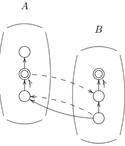
When there is an embedding of A in B, we note it A ⊑ B. Figure 2 gives an example of embedding ; the numbers correspond to moves of A (they are labels for the moves of B). The solid arrows are in ma, the dotted arrows in mB.

This allows us to derive from G a function sending strategies of A to strategies of B (this function is still called G) : if s is a strategy of A, G(s)’s answer to a move xa _{is the unique y}b _{such that x}a mB∩mA

−−−−−→ yb_{, where s’s} answer to a is b (mB∩mAis short for RB(mB)∩RB(mA), which is a modality of B).

Thus embeddings are related to the concept of sub-types : a strategy s on a game A can represent a term of the “type” A (as we saw for PCF). If B is a game in which A is embedded, the behavior of s is well defined as a strat-egy on B ; this means that every behavior allowed on A will also be allowed on B (in A, every possible action corresponds to an arrow of mA; in B, an arrow of mB∩ mAcorresponds to an action of B and at the same time to an action inherited from A). Thus B is a subtype of the more restrictive type A. Another way to see this is that B contains a (faithful) copy of A, which can be explored by following arrows of mA∩ mB in B. But strategies of B are also allowed to follow arrows of mB; by doing this, they switch to a new state, which is also in a copy of A. But it might be a different copy. On the example of figure 2, the only arrow of mB which is not also an arrow of mA switchs between two copies of A (which share the initial move 1). A strategy of A, when playing on B through the embedding, can only stay in

B A ❄❃❂❁ ✽✾✿❀₄ ❄❃❂❁ ✽✾✿❀₄ ❄❃❂❁✽✾✿❀₃ ❏❏ ❭❭ ✝✤ ✽ ❄❃❂❁ ✽✾✿❀₃ ❖❖ ❄❃❂❁ ✽✾✿❀₄ ❄❃❂❁✽✾✿❀₂ ❏❏ ❭❭ ✝✤ ✽ ❄❃❂❁ ✽✾✿❀₂ ❖❖ ❄❃❂❁ ✽✾✿❀₃ ❏❏ ❭❭ ✝✤ ✽ _❉❉ ❴ ❞ q ☎ ❄❃❂❁ ✽✾✿❀₁ ❖❖ ❄❃❂❁ ✽✾✿❀₂ ❏❏ ❭❭ ✝✤ ✽ ❄❃❂❁ ✽✾✿❀₁ ❏❏ ❭❭ ✝✤ ✽ ▲▲ Fig. _{2 – an embedding of A in B}

the same copy of A. Furthermore, it must answer based only on the label of the move ; it cannot, for example, distinguish between the two moves of B labeled by 2.

In this sense, embeddings enforce access control on B. Not only do they restrict the actions available (in the same way that a sub-type specifies a restriction on the actions of a term), they also restrict the information available to a strategy. These two types of restrictions will correspond to visibility and dependency, respectively.

2.4 Operations on games

We define A×B as (KA+KB, mA∪mB, IA∪IB, PA∨PB), where KA+KB is the obvious disjoint union on Kripke structures.

We define A ⇒ B as (KA+ KB, m, IB,¬PA∨ PB), where m is mA∪ mB, with additional arrows from every initial move of B to every initial move of A. Using ⇒ and ⊥ (the game with only one initial O-move, and all modalities the empty relation), we build the simple types as in the usual presentation of game semantics (using ⇒ for the arrow type). The difference is that here, types are actual games ; although very limited ones. Indeed a player can never backtrack to a previous position in the type ; this will be achieved by the following class of operators.

His a history operator if, for any game A, HA is defined in the following way :

– As the first step, for every initial move a of A, build a move in HA labelled by a (we are at the same time defining a cannonical embedding of A in HA). To each of these moves, associate a set of “bound” moves. The exact computation of this set is what differs from one history operator to another.

– Following steps : to every move xa _{built at the previous step, add} xa mA∪mH A

−−−−−−→ yb _{to HA for each a−→}m

Ab(thus one new move and two new arrows were constructed in HA).

Then, for each move x′a′ bound at xa_{, and for each a}′ m

−→A b′, add xa m_−→

HA y′b

′

and x′a′ −A→ y′b′ to HA. Here y′

is played by “calling” the bound move x′a′.

Compute then the sets of bound moves for the new moves y and y′ . They must be in the mHA branch of y (or y′) (the branch of a move being all moves in the unique path from an initial move to itself). Finally, for each new move y (or y′), and for each xa −−→ yA∗ b such that a−→ b, where m is a modality of A, add xm a m_{−→ y}b _{in HA. The} computation of the bound moves may not depend on these modalities, only on mAand mHA.

It is immediate that this defines an embedding of A in HA, with a total labelling function ; we still note it H. Another important property is that each move of HA is uniquely determined by its mHA branch, enriched by the modality mA.

2.5 Examples of history operators

The most restrictive history operator is I, in which no move is ever bound ; the game can only proceed by following arrows in A. Thus IA = A. On the contrary, the maximal history operator is $, in which the whole branch of a move is bound. For any history operator H, the moves in HA have a corresponding move in $A (they are uniquely determined by their branch). H simply cuts some branches of $, according to its restrictions on bound moves. This gives a cannonical embedding of every HA in $A, for every game A.

?, resp. !, are the history operators where all O-moves, resp. P-moves, are bound. The operator ? gives the player the right to backtrack, while forbidding the opponent to call a bound move. Thus, if a strategy on ?A, is asked to play in a larger game (say, $A) through an embedding, it will not “see” moves where the opponent called a bound move (in these cases, opponent switched to another copy of ?A).

on ?A. Indeed, when A is a simple type, this corresponds to the definition of innocent strategies of type A, in the usual presentation of game semantics.

In the figure 2, B is equal to (part of) the game ?A : the arrow of mB from 3 to 2 corresponds to calling the bound O-move 1 to play a new move labelled by 2.

C is the history operator such that, at a move x in CA, the mA branch of x (in CA) is bound. We formally define cellular strategies on a game A to be P-strategies on CA. Again this corresponds exactly to the original defi-nition. The simplicity of this definition, and its symmetry (moves of player and opponent are treated in the same way) pave the way for the symmetry on the syntax that we mentioned in the introduction.

To give a categorical structure on games, we will need an application operator which is less restricted than ⇒. This will be achieved by ”⊸”. A ⊸ B is built from A ⇒ B in a way similar to history operators, with one extra limitation.

The initial moves of A ⊸ B have only themselves as bound move. When appending a move y to x, if we are calling a bound move z, x becomes the (only) bound move at y. If not, y keeps the same bound moves that x had, with no addition (thus there will always be exactly one bound move). As an extra limitation, when calling a (the) bound move for the first time, we may only proceed to an (initial) move of A.

In words, to a move in A ⊸ B correspond two (distinguished) moves of A ⇒ B, one in B, and one in A, one of them being stored as the bound move. This gives the right to switch from one side to the other (the move of the now inactive side becoming the bound one). But we do not allow both moves to be in B, which is why we need the extra condition. Also note that only player has the right to switch (by induction, bound moves are always O-moves)4. We have obvious embeddings of A and B in A ⊸ B, with partial labelling functions.

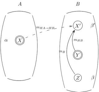
Figure 3 shows a move in the game A ⊸ B, where A = B = ⊥ ⇒ ⊥ ⇒ ⊥. The solid arrows correspond to the structure of A ⇒ B ; the dashed arrows correspond to a certain sequence (or history) of moves of A ⇒ B ; this history constitutes a move of A ⊸ B. The last move of each side in the sequence are the distinguished moves (noted by a double circle) ; here the move in B is the bound move. This information is sufficient to deduce the whole history (this is because A ⊸ B, as an history operator, is simple ; in particular it does not allow a state of A ⇒ B to be visited twice).

4

this assuming that O-moves and P-moves alternate in A and B, which is the case for all the games we consider, in particuliar simple types

A B ✴✳✲✱ ✭✮✯✰ ✴✳✲✱ ✭✮✯✰✤✣✢✜✘✙✚✛ ❖❖ ✫✫ ❭ ❩ ❳ ❯ ❙ _{P ▼}✴✳✲✱✭✮✯✰✤✣✢✜✘✙✚✛ ✴✳✲✱ ✭✮✯✰ ❖❖ ❲❲ ✤ ✴✳✲✱ ✭✮✯✰ ❖❖ ❲❲ ✤ ✴✳✲✱ ✭✮✯✰ ❖❖ ❢❢♥♥ ▼ P ❙ ❯ ❳ ❩ ❭

Fig. _{3 – a move in the game (⊥ ⇒ ⊥ ⇒ ⊥) ⊸ (⊥ ⇒ ⊥ ⇒ ⊥)}

3

Categorical structures

3.1 The category of games

Games form a category G, with maps from A to B being P-strategies of A ⊸ B.

Let σ and τ be maps from A to B and B to C, respectively. To define their composition, consider the game (A ⊸ B) ⊸ C ; to every move of this game corresponds a triple of moves in A, B and C. We have obvious embeddings of A ⊸ B, B ⊸ C and A ⊸ C in it, by taking as label the right pair of moves in this triple ; call them GA,B, GB,C and GA,C. Now GA,B(σ) ∪ GB,C(τ ) is a P-strategy of (A ⊸)B ⊸ C).

We first define a strategy σ|τ on (A ⊸ B) ⊸ C. To answer to an O-move x in C, GA,B(σ) ∪ GB,C(τ ) will follow an arrow coming from τ to either y′ in C or switch to B. In the second case, it will alternate arrows from σ and τ until it (possibly) emerges to a move y in A or C. If it does, we take y as the answer of σ|τ to x (in the other case, its answer is y′). We define the answer to an O-move of A in the same way.

Here, all the moves played in B were deterministic choices made by σ or τ ; the opponent on A ⊸ B, B ⊸ C only had a chance to play on A or C_{, corresponding to O-moves in A ⊸ C. Thus σ|τ , which was defined on} (A ⊸)B ⊸ C, indeed projects to a strategy on A ⊸ C, which we take as the composition of σ and τ , and note by σ; τ .

One can make the familiar observation here that σ and τ , which are both P-strategies on the respective smaller games, play respectively as player and opponent on B in the larger game.

The identity for this composition is the strategy of A ⊸ A which, to a move xa_{, responds by switching side and playing the (unique) move labelled} by a : the copycat strategy.

3.2 Functors

Only the results are presented for this section ; the proofs are given in the appendix.

The operator $ can be extended to an endofunctor of this category, using an embedding of A ⊸ B in $A ⊸ $B which can be inductively built. The contruction makes use of certain bound moves in $A and $B ; if these moves are also bound in the history operator H, then H is also an endofunctor. C, ? and ! all satisfy this condition.

3.3 The categorical structure of innocent strategies

We now state the general idea of the approach of [5], using these new definitions.

The starting point is the observation that, for any games A and B, ?(A ⇒ B) =!A ⊸?B ; this is true in particular when A and B are simple types. Additionally, ! and ? are a monad and a comonad (respectively), and along with other operators, they give G the structure of a model for full Intuitionistic Linear Logic.

The question is then to give a categorical meaning to the interaction of two innocent strategies σ and τ , which are now strategies on !A ⊸?B and !B ⊸?C. This is achieved by taking the image of these categorical maps by the functors ! and ?, respectively, and by invoking a law λ to build the following composition :

!A−→!!Aδ −→!?B!σ −→?!Bλ −→??C?τ −→?Cµ

which gives the composition of σ and τ as a map of !A ⊸?C (λ needs to verify some coherence properties, which correspond to being a distributive

law with respect to the monad and comonad).

3.4 The categorical structure of cellular strategies

Unfortunately, such a rich categorical structure cannot be given to cel-lular strategies with this approach. Indeed, we would need the equality C(A ։ B) = CA ։ CB, for some operator ։. We cannot take ⊸ for ։, because any simple type A with at least three consecutive moves (for example, ⊥ ⊸ ⊥ ⊸ ⊥) will allow strategies in A ⊸ A which are not cel-lular (if two moves are played on the left side and then one on the right side, A ⊸ A allows us to switch back to the left side and continue to the third move ; but doing so violates OP-visibility : we should only be allowed to play an initial move when switching side).

Moreover to define ։, we need to distinguish moves of CA according to mA, not just mCA (when on the right side, a move on the left side may only be bound if its label in A is initial (in A)). Thus ։ could only be defined on the image of C, and not as a general operator on games.

Still, our generalization has brought us some isight into this matter. Indeed, for every history operator H, we can show an embedding of H(A ⊸ B_{) into $A ⊸ $B (call this embedding G}H) . this allows us to define, in categorical terms, the composition of strategies corresponding to any history operators : if σ and τ are respectively strategies on H(A ⊸ B) and H′

(B ⊸ C), we can build the following diagram :

$A GHσ

−−−→ $B−−−→ $CGH′τ

Which gives us the composition of σ and τ as a strategy of $A ⊸ $B. Compared to the diagram for innocent strategies, the result is weaker since the composition is in a bigger game ; but this results applies to more than just innocent strategies. In particular, we can describe the composition of innocent strategies with cellular strategies.

The next section will, formally, give a syntactical equivalent to this result.

4

Game semantics for the generic syntax

4.1 Preliminary

To give the semantics of terms of the generic syntax, we need to extend to these terms some standard notions. For concision we only sketch this section.

For a term t, if we remove all (u : t′

) except when u has just been defined (with a subterm tu1...un

with u = ui), we obtain a basic lambda-calculus term, which can be well typed in the usual sense. If this is the case, for every (u : t′

) we previously removed, we can check if it is “compatible” with this type, by putting it back into t, just after u is defined, in place of any existing (u : t′′

). If all such (u : t′

) are compatible, we say that t is well typed. This gives us a simple type for t.

For example t′

1 and t′2 are well typed, with the same types as t1 and t2. We also assume a notion of normal form for terms of the generic syntax.

4.2 Game semantics

We now give a game semantics for the terms in the generic syntax. Let t be a term which is closed, in normal form and well typed. Let A be the game corresponding to its simple type. We inductively define a

P-strategy JtK on $A for t. We do this while associating subterms of t to the moves reachable by this strategy.

– First step : t is associated to the initial (opponent) move of $A. – Next steps, first case : if a subterm of the form λx1. . . xn.t′ was

asso-ciated to a move z at the previous step, then it was an O-move (by induction), and t′

is of the form xu1...un

(v1 : t1) . . . (vm : tm) (this is because t is in normal form ; the only thing we needed here was that t′

starts with a variable x).

Now, if x is one of the xi, the strategy answers by following the arrow of mA ∩ m$A corresponding to xi (this is a choice in A, given by the position of the type of xi in the type A of t), and we associate t′

= xu1...un

(v1 : t1) . . . (vm: tm) to that move.

If x is not one of the xi, there is a move in the mA branch of z to which we associated a subterm of the form λy1. . . yr.t′′, with x = yj. This move is bound at z ; the strategy’s answer is to call this move. Again we associate t′

to the reached move. – Next steps, second case : if a subterm of the form

(t′)u1...un

(v1: t1) . . . (vm: tm)

was associated to a move z at the previous step, then it was a P-move (by induction), and t′

is a variable x (normal form). Let z′ be a move such that z m$A

−−−→ z′

. The move z′

corresponds to one of the possible behaviors of x, which is a function played by the opponent (by definition, the strategy JtK must contain all arrows like z−−−→ zm$A ′

, to distinguish between these possible behaviors).

The move which justifies z′

(the unique move obtained by following m−_A1) indicates when in the interaction this argument was named, and the label of z′

distinguishes between the different arguments named at that move. This uniquely determines an argument name u′′

. If there is a matching (u′′

: t′′

)5 we associate t′′ to z′

. (If there is no matching (u′′

: t′′

), the strategy will have no answer if opponent plays z′ : this corresponds to the default value of Ω in the environment).

This shows the symmetry between argument and function names, since $A is absolutely symmetric between player and opponent.

It is clear that, for every simple type A, and every strategy s on $A, we can also gives a term corresponding to s by this method.

4.3 History operators as typing methods

This approach seems to single out the history operator $. But, since we have embeddings of every HA into $A, this also give a syntax to strategies

5

We take the latest occurence of (u′′ _{: t}′′_{) in the m}

$A branch, which is what the

of HA. Moreover, the different history operators are obtained from $ simply by restricting the sets of bound moves. By definition of history operators, these restrictions may only depend on the m_$A branch (along with the mA structure on this branch), which corresponds exactly to a prefix of the term. This means that the restrictions enforced by H can be checked statically on the terms : it can be seen as a typing method. This easily gives an exact correspondence between terms “well typed according to H” (with the pre-vious meaning), and strategies of HA (with A any simple type).

This does not necessarly mean that these typing methods can be effi-ciently computed ; we would have to impose further restrictions on history operators for this to be true (with our current definition, the selection of the bound moves could be the result of a non-computable function...). The reason for this (possible) inefficiency is that terms can match a branch of the execution of arbitrary length.

But for the operators we considered, the typing methods are indeed simple. For example, a term is well typed according to ? if “(u : t)” only appears just after u is defined, as in the standard way of passing arguments (this because defining u is done at a player move, which is never bound in ?A).

The case of C is more interesting : its typing method is obtained simply by taking the method described in section 1 (for the specific syntax), and treating the argument names in exactly the same way as function names (they are put on the stack structure of the environment). The information granted to a term by these bound argument names is exactly the same that would have been granted by the recordings. This result is quite striking when one considers how unnatural the restrictions for storing and passing recordings are.

5

Future work

Some further generalizations of embeddings and history operators can be investigated.

In embeddings, the third condition, which imposes in particular that justifying moves be in the mA branch, could be removed. This would allow a player to place the opponent in an arbitrary state (a generalization of the backtracking which a term would be subjected to when β-reduction duplicates one of its subterms). This would correspond to the player choosing the opponent’s move until a certain point - the equivalent of a debugging software modifying the values of variables in another function. The resulting notion of embedding would then be entierly local.

History operators include all the transformations on games that we were interested in, while being sufficient for the result we wanted to prove. But

they are not the weakest conditions needed to obtain those results. A better method (which was our initial approach) is to define more basic operators on games, as building blocks for the others. For example a “travel” opera-tor would build moves for each branches of the existing game (the resulting game having the structure of a tree).

These basic operators can be seen as transformations on modal logic formulas ; an operator on games would then build the image of a game A by building a new structure B which inherits the modality mA, and then define mB by applying a transformation on the formula of mA (some modalities can be described by a formula).

The motivation for this approach is that, as long as the operations used are simple enough, the decidability results on modal logic ([6]) could be used. It is possible to decide if a formula is true on a given structure (which could allow to check that a strategy verifies properties like innocence). But, given a formula, it is also possible to decide if there exists a structure on which the formula is verified (at some state), through the tableau method. This could allow to check a general property of HA, for all A. This method relies on the fact that two states are indistinguishable if the same paths can be followed from them (with respect to modalities and atomic propositions en-countered). This is compatible with our definitions for games, in particular the property that moves in HA are uniquely determined by their mAbranch.

Finally, to make full use of the generality of history operators, we intend to study their effects on arbitrary games. The generic syntax was obtained by studying only HA, where A is a simple type ; in [5], !?A was considered, not its strategies (only those corresponding to ?A). But, in the same way that types can be seen as (linear) games, any game can be seen as the extended ”type” of its strategies ; we showed for example that the game HA is a type in the usual sense for strategies of $A (whereas the usual presentation only made explicit the simple type A for the same strategies). This hints at a way to build more precise types, expressing, statically, a more precise access control (which would benefit from our further generalizations of embeddings and history operators). It would also be interesting to apply a Curry-Howard isomorphism to these terms. This will be the subject of our next investigations.

Conclusion

As a study of semantics, our generalization of games has allowed us to describe general concepts of embeddings and history operators, which are interesting in their own right. They make apparent some important notions which are implicit in the usual presentation, such as the fine grained access

control imposed on interacting strategies, and the symmetry of visibility and dependency.

But these results have counterparts in languages. Indeed, the generic syntax, by its tight correspondence to the semantical object $, often makes regularities of this object apparent - statically - on the terms.

Thus the study of game semantics can indeed help discover new lan-guages.

A

Functors on the category of games

Let H be a history operator ; we want to give a sufficient condition to be able to expand H to an endofunctor in the category G.

We first need to define a strategy of HA ⊸ HB for every strategy in A ⊸ B. To do this we attempt to define inductively an embedding of A ⊸ B in HA ⊸ HB.

– An initial move Y of HA ⊸ HB corresponds to an initial move y of HB, labelled by b in B (with itself as bound move) ; we label it by the initial move b in A ⊸ B, with itself as bound move.

– Let X be a move in HA ⊸ HB, labelled by xa _{in HA (a is x’s label} in A ; the case where x ∈ HB will be defined symmetrically), with bound move Y labled by yb _{in HB.}6

Suppose that we have already labelled X by a move α of A ⊸ B, with bound move β labelled by c in B (α is necessarly labelled by a). We note that α is uniquely determined by its m_A⊸B branch, and, by conditions (2) and (3) of the embedding we are building, the moves of this branch correspond exactly to the m_A⊸B branch of X in HA ⊸ HB. Thus β is the label in A ⊸ B of a move Z in the mA⊸B branch of X, with Z labelled by zc _{in HB.}

We can now label (some) moves reachable from X. First, for all arrows α_{−−−−→ α}mA⊸B ′

(in A ⊸ B) with α′

labelled by a′ in A, there is exactly one X′

in HA ⊸ HB such that X mA∩m_{H A⊸HB}

−−−−−−−−−−→ X′ and such that X′

is labelled by a′

(by the embedding of A in HA, since α−−→ αmA ′

). We label X′ by α′

, and X _{−−−−→ X}mA⊸B ′ . Secondly, for every α_{−−−−→ β}mA⊸B ′

with β′

labelled by b′

in B, we have β mB

−−→ β′

(with β the bound move of α and the label of Z, as before). If Z is bound at Y (in HB), or if Z = Y , there is exactly one Y′

in HA ⊸ HB such that Z−−→ YmB ′

and Y −−−→ YmHB ′

(which means that X_{−−−−−−→ Y}mH A⊸HB ′

). We label Y′ by β′

, and X _{−−−−→ Y}mA⊸B ′ .

The situation is summed up in the figure 4 : the dashed arrow can be built if the two solid arrows exist. X (with bound move Y ), is the current position in HA ⊸ HB, while α (with bound move β), is the current position in A ⊸ B.

The construction will succeed if, in the last case, Z is always bound at Y when Z 6= Y .

Let H be any history operator such that the previous construction suc-ceeds. We will now prove that H is a functor.

Let σ and τ be P-strategies on A ⊸ B and B ⊸ C ; we note Hσ and Hτ their images in HA ⊸ HB and HB ⊸ HC (even though Hσ was already

6

We do not give the details for the case where X is initial with bound move itself, but it can easily be deduced from the general case.

A B ●❋❊❉ ❅❆❇❈_X′ _β′ α ●❋❊❉❅❆❇❈❄❃❂❁✽✾✿❀X m_{H A⊸HB} ✶✶ ❧ ❥ ✐ ❣ ❢ ❞ ❝ ●❋❊❉ ❅❆❇❈❄❃❂❁✽✾✿❀_Y mH B ●● ❄❃❂❁ ✽✾✿❀_Z mB ❉❉ β

Fig. _{4 – Building a new move X}′ _{in HA ⊸ HB} defined as the image of σ in H(A ⊸ B) ; no confusion will arise).

Consider now the composition of Hσ and Hτ in (HA ⊸ HB) ⊸ HC. Suppose the external opponent plays in HC ; then the composition will follow an arrow of Hτ , which will stay in the same copy of B ⊸ C, then possibly alternate arrows of Hσ and Hτ , staying in the intersection of their copies of B ⊸ C and A ⊸ C, which we can see as a single copy of (A ⊸ B) ⊸ C. Thus their answer will be the same as H(σ; τ ), by the embedding of A ⊸ C in HA ⊸ HC (which is compatible with the two other embeddings, meaning that two moves in HA ⊸ C and HA ⊸ HB with the same label in HA, for example, will have the same label in A by the corresponding embeddings given by H).

This shows that H, as an operation on maps in the category of games, preserves composition. Since the image by H of the identity is clearly the identity, H defines a functor.

Proposition A.1. The history operator$ defines a functor on G

D´emonstration. The construction shown previously succeeds ; indeed, using the same notation as before, Z is always in the mHB branch of Y , and thus bound at Y .

Proposition A.2. The history operatorC defines a functor on G

D´emonstration. Because Z corresponds to β in A ⊸ B, it is always in the mB branch of Y , and thus it is bound at Y .

Again a result on cellular strategy is made almost trivial once we have the general case.

Proposition A.3. The history operators ? and ! define functors on G

D´emonstration. If X is on the left side of ?A ⊸?B (if it corresponds to a move in ?A), then Z is on the right side, it which case it is bound in ?B (as an O-move of ?B). If X is on the right side, this does not work, because Z now corresponds to a P-move of ?A, which is not bound (recall that the polarity of moves is reversed on the left side of ⊸). But if we follow m−_?A⊸?B1 from X, as long as we stay on the right side, every arrow we follow is also in mB : player will never call a bound move because it plays according to a strategy defined on A ⊸ B, and player is the only one able to call bound moves in ?B. Thus we stay in the same copy of A ⊸ B until we switch side, which happens at Z (opponent cannot switch side, and β was the last move on the left side of A ⊸ B in the branch of α). Thus Z = Y .

For !, the argument is symmetric : Z is bound if it is on the left side, and only player can call bound move in the copy of !A (with the polarity inversion), yielding Z = Y if Z was on the right side.

R´

ef´

erences

[1] P.-L. Curien and H. Herbelin. Abstract machines for dialogue games.

Panoramas et synth`eses, 2009. To appear.

[2] J. M. E. Hyland and C.-H. L. Ong. On full abstraction for PCF : I, II

and III. Information and Computation, 163 :285-408. 2000.

[3] S. Abramsky, R. Jagadeesan and P. Malacaria. Full Abstraction for

PCF. information and Computation Vol. 163, pages 409-470. 2000. [4] R. Harmer. Cellular strategies and innocent interaction. 2008. To

ap-pear

[5] Russ Harmer, Martin Hyland and Paul-Andr´e Melli`es. Categorical

com-binatorics for innocent strategies. LICS’07. 2007.

[6] P A. Bonatti, C. Lutz, A. Murano and M Y. Vardi. The Complexity of

Enriched µCalculi. Logical Methods in Computer Science Vol. 4 (3 :11), pages 1-27. 2008