HAL Id: hal-00906361
https://hal.archives-ouvertes.fr/hal-00906361
Submitted on 19 Nov 2013
HAL is a multi-disciplinary open access
archive for the deposit and dissemination of
sci-entific research documents, whether they are
pub-lished or not. The documents may come from
teaching and research institutions in France or
abroad, or from public or private research centers.
L’archive ouverte pluridisciplinaire HAL, est
destinée au dépôt et à la diffusion de documents
scientifiques de niveau recherche, publiés ou non,
émanant des établissements d’enseignement et de
recherche français ou étrangers, des laboratoires
publics ou privés.
Uncertainty Analysis of Phast’s Atmospheric Dispersion
Model for Two Industrial Use Cases
Nishant Pandya, Nadine Gabas, Eric Marsden
To cite this version:
Nishant Pandya, Nadine Gabas, Eric Marsden. Uncertainty Analysis of Phast’s Atmospheric
Disper-sion Model for Two Industrial Use Cases. Chemical Engineering Transactions, AIDIC, 2013, vol. 31,
pp. 97-102. �10.3303/CET1331017�. �hal-00906361�
Open Archive TOULOUSE Archive Ouverte (OATAO)
OATAO is an open access repository that collects the work of Toulouse researchers and
makes it freely available over the web where possible.
This is an author-deposited version published in :
http://oatao.univ-toulouse.fr/
Eprints ID : 9946
To link to this article :
DOI:10.3303/CET1331017
URL : http://dx.doi.org/10.3303/CET1331017
To cite this version :
Pandya, Nishant and Gabas, Nadine and Marsden, Eric Uncertainty
Analysis of Phast’s Atmospheric Dispersion Model for Two
Industrial Use Cases. (2013) Chemical Engineering Transactions,
vol. 31 . pp. 97-102. ISSN 1974-9791
Any correspondance concerning this service should be sent to the repository
administrator: staff-oatao@listes-diff.inp-toulouse.fr
Uncertainty Analysis of Phast’s Atmospheric Dispersion
Model for Two Industrial Use Cases
Nishant Pandya
a, Nadine Gabas*
a, Eric Marsden
baUniversité de Toulouse; INPT, UPS ; Laboratoire de Génie Chimique; 4 allée Emile Monso, BP 84234, 31432 Toulouse France
b
Institut pour une Culture de Sécurité Industrielle, 6 allée Emile Monso, BP 34038, 31029 Toulouse, France nadine.gabas@ensiacet.fr
We have undertaken an uncertainty analysis of the dispersion model of a widely used tool for consequence assessment, comparing the level of output variability observed for an accident investigation use-case (where input variables concerning the release conditions are uncertain) and a risk prevention use-case (where the effect of uncertainty in internal model parameters is evaluated). As expected, for the two flammable and two toxic materials studied, uncertainty for the risk prevention use-case is significantly lower than that for accident investigation. We have identified the release conditions which lead to the highest level of variability in model outputs.
1. Introduction
Consequence estimations of accidental releases of hazardous gases have a significant impact on land use planning around industrial plants and on the choice of risk prevention and mitigation barriers. Atmospheric dispersion simulations are dependent on a significant number of variables (source term, weather conditions) as well as internal parameters of the dispersion model. Uncertainty in these variables and parameters has a significant impact on model outputs (concentration at a given distance, toxic dose, etc.). Consultation of stakeholders and decision-makers would be improved by a better understanding of how uncertainty in model inputs propagates to outputs. Moreover, there is growing regulatory and stakeholder demand for information on uncertainties in safety case and environmental impact assessment studies. This subject has motivated significant amounts of research over the last two decades (Shankar Rao, 2005; Hanna, 1993; Argence et al., 2010; Demaël, 2007; for example). Whilst the quantification and the interpretation of uncertainty in models used in the air quality community are widespread, this practice is very limited in the field of industrial risks studies. Moreover, previous works are limited to a few sources of uncertainties and to specific case-studies.
This paper presents our work on an uncertainty analysis of the outdoor dispersion model of Phast v6.7 (Witlox, 2010), one of the most comprehensive computer programs for the modeling of accidental releases, used by companies and the competent authorities. The analysis concerns 10 to 30 min continuous releases of two toxic and two flammable materials, examining the impact of representative variation of the significant variables and internal model parameters. We investigate two different industrial use cases of the software: accident investigation and risk prevention.
2. Uncertainty analysis
When model outputs are used for decision-making, good practice suggests providing best estimates together with a quantitative estimate of the level of uncertainty (such as a confidence interval). Uncertainty analysis involves evaluating the robustness of model predictions, given the various uncertainties which affect the model input variables and parameters.
1. Quantifying the uncertainty in input variables (release rate, orifice diameter, wind speed, etc.) and model parameters (in Phast, parameters such as averaging time) in the form of probability density functions; 2. Propagating the uncertainty from the inputs to the outputs, using Monte-Carlo techniques (large number of model evaluations, with variables and parameters taken stochastically from their input distributions); 3. Presenting the results to decision-makers using various tools, such as histograms or quantitative measures such as the coefficient of variation (CV) or confidence intervals.
Historically, the large number of model executions required for a quantitative uncertainty analysis has been an obstacle to its use. Modern computer power and increasing demands from decision-makers, have led to more widespread use.
3. Selected hazardous materials
We have selected four materials: two toxic (nitric oxide and ammonia) and two flammable (methane and propane) because they cover a range of common scenarios in safety reports. They are stored under various conditions and, given their physico-chemical properties, are likely to exhibit different behavior during dispersion. Nitric oxide (NO) is a neutral gas whose behavior is similar to that of ambient air. It is usually stored in a pressurized tank. Ammonia (NH3) is usually stored in the liquid phase in pressurized
vessel. After its emission, a two-phase flow occurs forming a cloud composed of vapor and very fine droplets that do not fall to the ground. The droplets evaporate quickly, cooling the air, generating a cold mixture of air and ammonia, denser than the ambient air, even though pure gaseous ammonia is lighter than air at ambient temperature. An emission plume of methane (CH4) at ambient air temperatures is
buoyant because methane has a lower molecular weight than the ambient air. It is extremely flammable over a range of concentrations from 4.4 to 16.5 % in air. Propane (C3H8) is liquid when stored under
pressure and flashes immediately upon release to the atmosphere. Upon accidental release of liquefied propane, a two-phase mixture is released with about 75 % of liquid content. The droplets in the two-phase mixture evaporate quickly. Propane is flammable over a range of concentrations, from 2 to 9.5 % in air. 4.
Methodological approach
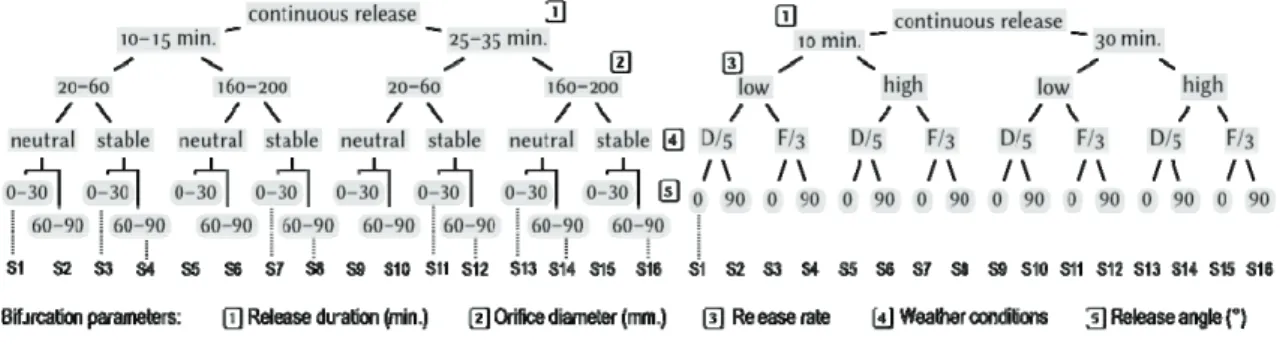
In this paragraph, we describe the strategy adopted to select the release scenarios for each product and the methodology that we have developed to undertake an uncertainty analysis of Phast. In previous work (Pandya et al., 2012), we have undertaken a sensitivity analysis of Phast on a more limited range of products. The previous research showed that certain input variables have a significant impact on the physical phenomena: for instance, the dispersion of a release with a high release rate is very different in nature to a low release rate. In order to understand the phenomena in detail, we have decided to analyse separately scenarios with different physical phenomena. We have therefore chosen four “bifurcation parameters” (release duration, orifice diameter, weather conditions, release angle) and studied separately scenarios with “high” and “low” values. This leads to a “scenario tree” of 16 scenarios for each product as shown in Figures 1 and 2.
Figure 1: Scenario tree: “accident investigation” use Figure 2: Scenario tree: “risk prevention” use
4.1 Analysis strategy
We have undertaken two types of uncertainty analyses, which aim to provide understanding of two industrial use-cases of the release and dispersion models in Phast:
1. “Accident investigation” use, or release conditions uncertainty analysis: we assume that the user wishes to model a historical accident, for which he has some (uncertain) information on the release conditions and weather conditions, and wishes to assess the level of confidence he can place in his simulations, given these “irreducible” input uncertainties.
2. “Risk prevention” use, or model uncertainty analysis: we assume that the user is working on a risk assessment for regulatory purposes or for process design. Such simulations are often undertaken according to a certain number of modeling guidelines, which impose stereotypical assumptions on the release conditions (specific wind speeds, specific orifice diameters) in order to increase the homogeneity of risk assessments across a regulatory domain. This type of uncertainty analysis aims to assess the level of confidence in the model outputs given the uncertainty one has on the values of various internal Phast parameters (uncertainty inherent to the use of the specific model).
4.1.1 Accident investigation use-case
In this paragraph, we examine the influence of uncertainty in “physical” parameters of the scenario. Table 1 shows the parameters studied. Ranges for the parameters were selected with expert Phast users to be representative of uncertainty ranges when modeling an accident. All other variables and parameters are maintained at their default values. NH3 and C3H8 are stored as saturated liquid and NO and CH4 are stored
as pressurized gas at 10 bar absolute.
Table 1: Variables and parameters for the “accident investigation” use case
Parameter Nomenclature / Unit Distribution Range of variation
Tst Storage temperature / K triangular NH3: [263.15 – 283.15] centered at 273.15 K
NO, CH4, C3H8: [273.15-293.15] centered at 283.1K
Lh Liquid height / m uniform [12.75 - 17.25]
Ta Atmospheric temperature / K triangular [282.65 - 287.65] centered at 285.15 K
Pa Atmospheric pressure / Pa uniform [0.99·105 - 1.035·105]
Ha Relative atmospheric humidity / - triangular [0.55 - 0.85] centered at 0.7
DO Orifice diameter / m triangular
Value 1: [0.02 - 0.06] centered at 0.04
Value 2: [0.16 - 0.20] centered at 0.18 Durmax Maximum release duration / s uniform Value 1: [300 - 900] Value 2: [1500 - 2100]
angle Release angle / degree uniform Value 1: [0 - 30] Value 2: [60 - 90] SC Stability Class / - discrete Neutral: [10 % C/D, 80 % D, 10 % E]
Stable: [10 % E, 80 % F, 10 % G] ua Wind speed / m·s-1 uniform Neutral: [4 - 6] Stable: [1.5 - 3]
Sflux Solar radiation flux / W·m-2 triangular Neutral: [250 - 1000] centered at 500 Stable: [0 - 500] centered at 250 ZR Release height above ground/ m uniform [1 - 10]
Z0 Surface roughness length / m triangular [0.5 - 1.5] centered at 1
4.1.2 Risk prevention use-case
In this part of the analysis, we vary only internal parameters of Phast’s dispersion model, and keep all other variables and parameters at their default values. The parameters studied and their distributions are given in Table 2; bifurcation parameters are listed in Table 3. In the absence of information on the “real” level of uncertainty on these internal parameters (some of which have been calibrated from experiments, others taking values given in the scientific literature, and some having little scientific justification), we have studied the effect of variations of ±10 % of the variation range allowed in Phast, around the default value. For most parameters, we have examined normal distributions around the default value in Phast, with a standard deviation selected such that 99 % of values are within two standard deviations of the mean. The parameters CDa and ! have a default value of 0 and cannot adopt negative values, so a normal distribution
Table 2: Studied parameters and values: “Risk prevention” use case Parameter Default value Distribution !" (mean) #• (std dev.) $%"(jet entrainment parameter)" 0.17 normal 0.17 0.0085
$&"(cross-wind entrainment parameter)" 0.35 normal 0.35 0.0175
CDa (drag coefficient of plume in air) 0 exponential '"= 69.2
("(dense cloud side entrainment parameter)" 0 exponential '") 34.6
CE (cross-wind spreading parameter) 1.15 normal 1.15 0.0575
epas (near-field passive entrainment parameter) 1 normal 1 0.05
ru pas
(max cloud/ambient velocity parameter) 0.1 normal 0.1 0.005 rropas (max cloud/ambient density parameter) 0.015 normal 0.015 0.00075
rEpas(max non-passive entrainment fract° param.) 0.3 normal 0.3 0.015
Ri* pas
(max Richardson number) 15 normal 15 0.75 rtr
pas
(distance for phasing in passive entrainment) 2 normal 2 0.1 Ri (Richardson number for lift-off criterion) -20 normal -20 1 rquasi (quasi-instantaneous parameter) 0.8 normal 0.8 0.04
Ripool (Richardson for passive transition above pool) 0.015 normal 0.015 0.00075
Entpool (pool vaporisation entrainment parameter) 1.5 normal 1.5 0.075 tavtox (s) (averaging time for toxic release) - uniform For 10 min release: [540 – 660]
For 30 min release: [1620 – 1980]
Table 3: Bifurcation parameters and values: “risk prevention” use case
Parameter Unit Value1 Value2
Durmax s 600 1800
DO m 0.04 0.18
Release angle degree 0 90 Weather
conditions
SC/ ua - / m·s-1 D/5 F/3
Sflux W·m-2 500 for D/5 250 for F/3
4.2. Methodology
In order to propagate the uncertainty from the input variables and parameters to the outputs, we have undertaken Monte-Carlo stochastic analyses using 20,000 runs of Phast for each scenario. The number of runs was decided during preliminary runs, as a compromise between execution time and repeatability of the uncertainty analysis. We have developed testbed software which is able to execute multiple parallel Phast instances in “batch mode”, and retrieve the results in a central database. Using a total of 20 virtual machines running Phast (on 5 physical servers), the 20,000 runs take approximately 12 h to run, depending on the complexity of the scenario. The testbed interfaces with the Simlab (2011) package to implement stochastic sampling and sensitivity analysis. This experimental work has led us to execute Phast more than a million times over a 12 month period.
5. Results and discussion
The results concern continuous discharges from a storage tank (“leak” module of Phast). The cloud is assumed to progress in an open field (no impingement). We have investigated concentrations at downwind distances ranging from 50 m to 200 m (for flammable releases) and 500 m to 2 km (for toxic releases); these correspond to typical distances of interest. Outputs for toxic releases are calculated at the reference height of 1.5 m (used in French safety case studies), whereas for flammable releases they are measured at the centre of the cloud (indeed, safety case studies mostly aim to estimate the flammable volume and thus take the point of maximal concentration as a reference). In all simulations, the “core averaging time” has been set to the “averaging time”. For flammable materials, tav is set equal to 18.75 s (no
time-averaging). The results are expressed in terms of coefficient of variation (CV) of each output variable’s distribution, which is defined as the ratio between the standard deviation and the mean, expressed as a
percentage. It is a convenient quantitative measure of the dispersion of the distribution, i.e. of the level of uncertainty in model predictions.
5.1 Comparing uncertainty for the two industrial use cases
Figure 3 shows the mean CV of the output concentrations for the 16 scenarios we investigated for products NH3, NO, CH4 and C3H8 according to both use cases. The results confirm that, as expected, the
level of uncertainty in the output is always higher for “accident investigation” use cases (where release conditions vary) than for “risk prevention” use cases (where only internal model parameters vary, representing the “model uncertainty”).
Concerning toxic releases, risk analysis use cases lead to a mean CV ranging between 2 % and 7 %, whereas accident-investigation use cases give CV ranging between 30 % and 65 %. Concerning flammable releases, risk analysis use cases give mean CVs ranging between 3 % and 4 %, much lower than accident-investigation use cases with CV ranging between 25 % and 40 %.
Figure 3: Mean CV of all scenarios for each material, per use case (AI: Accident Investigation, RP: Risk Prevention)
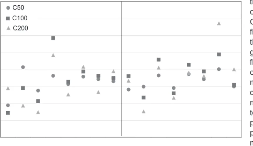
5.2 Release conditions which lead to the highest level of uncertainty
We have identified which release conditions lead to the highest output variability. Figure 4 represents the CV of concentration outputs for all NO and NH3 scenarios, for the “risk prevention” use case. The highest
values of CV are found for vertical NO releases in stable weather conditions, in particular with high release rates (scenarios NO-8 and NO-16). During a vertical NO release, the cloud rises above the ground and remains buoyant. The ground concentration at different distances is lower for a vertical release than for a horizontal release, and is sensitive to small variations in model parameters. For other NO and NH3 releases, CV
remains less than 5 %.
Figure 4: CV of concentrations for NO and NH3 scenarios (risk prevention use-case)
In the case of a two phase ammonia release, the cloud is denser (cold gas with creation of aerosol) than for NO, and thus always remains close to the ground, leading to less fluctuation of measured concentrations at the reference height, and thus to low values of CV.
If we examine uncertainty as a function of the distance from the release point, we observe in scenarios NO-8 and NO-16 that the CV is higher in the near field (C500 output) than the far field. Sensitivity analysis of this scenario (identifying the parameters which have the greatest contribution to total output uncertainty) shows (Pandya et al., 2012) that the !2 parameter is the greatest contributor to uncertainty (note however
that the influence of !2 decreases as one moves farther from the release point, the value of CV also decreases. This is compatible with the hypothesis that when the cloud transitions to passive dispersion, the level of uncertainty in the outputs decreases.
Concerning the releases of
flammable products (cf.Figure 5), the level of uncertainty is low (CV generally below 4 %). Indeed, for
flammable releases, the
concentration of interest is the maximum concentration at the centre of the cloud, which is mostly dependent on the source term, and not on the dispersion
phase (the internal Phast
parameters we have studied mostly impact the dispersion phase).
Figure 5: CV of concentrations for methane and propane scenarios (risk prevention use-case)
6. Conclusion
For the two flammable and two toxic materials studied, we have confirmed that model uncertainty is significantly lower than uncertainty resulting from variation in source term and weather conditions. We have identified the release conditions which lead to the highest level of model uncertainty; exceptionally high values have been found for vertical releases of NO in stable weather conditions with high release rates.
Quantitative information concerning the level of uncertainty impacting consequence estimations can help risk analysts understand the degree of confidence they can place in modeling results. When comparing the effect of different risk reduction investments, it tells decision-makers whether the investment ranking is robust, given various modeling uncertainties. When modeling results inform land-use planning decisions, uncertainty analysis provides local government officials and other stakeholders with information which can help to arbitrate between different strategies. Until modeling tools integrate uncertainty analysis tools, our work on families of release scenarios gives an indication of the level of uncertainty one can expect for a given product and for given release conditions.
Acknowledgments
The authors would like to acknowledge valuable technical assistance from experienced Phast users working for the industrial sponsors of this work, Total. We also thank DNV Software for useful feedback.
References
Argence S, Armand P, Yalamas T, Deheeger F, Brocheton F, Buisson E., 2010, Investigation of different methodologies to characterize and propagate uncertainties in atmospheric dispersion modelling : application to long-term impact assessment, Proceedings of the 13th Conference on Harmonisation within Atmospheric Dispersion Modelling for Regulatory Purposes, 80-84, Paris.
Demaël E., 2007, Modelling of atmospheric dispersion in complex areas and linked uncertainties, PhD thesis (in French), Ecole Nationale des Ponts et Chaussées, France.
Hanna S.R., 1993, Uncertainties in air quality model predictions. Boundary-layer meteorology, 62, 3-20. Pandya N., Gabas N., Marsden E., 2012, Sensitivity analysis of Phast’s atmospheric dispersion model for
three toxic materials (nitric oxide, ammonia, chlorine), Journal of Loss Prevention in the Process Industries, 25: 20-32.
Shankar Rao, K., 2005, Uncertainty analysis in atmospheric dispersion modelling. Pure Appl. Geophys, 162, 1893-1967.
Simlab, 2011, Software package for uncertainty and sensitivity analysis. Joint Research Centre of the European Commission. simlab.jrc.ec.europa.eu, accessed July 2011.
Witlox H., 2010, Overview of consequence modelling in the hazard assessment package Phast, Paper 7.2, 6th AMS conference on applications of air pollution meteorology, 17-21 January 2010, Atlanta, USA.
C50 C100