The Effects of Thermostat Setting on Seasonal Energy Consumption at the CCHT Research Facility

(1)

Publisher’s version / Version de l'éditeur:

Vous avez des questions? Nous pouvons vous aider. Pour communiquer directement avec un auteur, consultez la

première page de la revue dans laquelle son article a été publié afin de trouver ses coordonnées. Si vous n’arrivez pas à les repérer, communiquez avec nous à PublicationsArchive-ArchivesPublications@nrc-cnrc.gc.ca.

Questions? Contact the NRC Publications Archive team at

PublicationsArchive-ArchivesPublications@nrc-cnrc.gc.ca. If you wish to email the authors directly, please see the first page of the publication for their contact information.

https://publications-cnrc.canada.ca/fra/droits

L’accès à ce site Web et l’utilisation de son contenu sont assujettis aux conditions présentées dans le site LISEZ CES CONDITIONS ATTENTIVEMENT AVANT D’UTILISER CE SITE WEB.

Research Report (National Research Council of Canada. Institute for Research in

Construction), 2005-02-14

READ THESE TERMS AND CONDITIONS CAREFULLY BEFORE USING THIS WEBSITE.

https://nrc-publications.canada.ca/eng/copyright

NRC Publications Archive Record / Notice des Archives des publications du CNRC :

https://nrc-publications.canada.ca/eng/view/object/?id=344f31a2-8d67-4c5a-84bd-488fe7a18f59 https://publications-cnrc.canada.ca/fra/voir/objet/?id=344f31a2-8d67-4c5a-84bd-488fe7a18f59

NRC Publications Archive

Archives des publications du CNRC

For the publisher’s version, please access the DOI link below./ Pour consulter la version de l’éditeur, utilisez le lien DOI ci-dessous.

https://doi.org/10.4224/20378071

Access and use of this website and the material on it are subject to the Terms and Conditions set forth at

The Effects of Thermostat Setting on Seasonal Energy Consumption at

the CCHT Research Facility

(2)

Canadian

Centre

canadien

des

for Housing Technology

technologies résidentielles

The Effects of Thermostat Setting on Seasonal Energy

Consumption at the CCHT Research Facility

Manning M.; Swinton, M.C.; Szadkowski, F.; Gusdorf J.; Ruest K.

(3)

The Canadian Centre for Housing Technology (CCHT)

Built in 1998, the Canadian Centre for Housing Technology (CCHT) is jointly operated by the National Research Council, Natural Resources Canada, and Canada Mortgage and Housing Corporation. CCHT's mission is to accelerate the development of new technologies and their acceptance in the marketplace.

The Canadian Centre for Housing Technology features twin research houses to evaluate the whole-house performance of new technologies in side-by-side testing. The twin houses offer an intensively monitored real-world environment with simulated occupancy to assess the performance of the residential energy technologies in secure premises. This facility was designed to provide a stepping-stone for manufacturers and developers to test innovative technologies prior to full field trials in occupied houses.

As well, CCHT has an information centre, the InfoCentre, which features a showroom, high-tech meeting room, and the CMHC award winning FlexHouse™ design, shown at CCHT as a demo home. The InfoCentre also features functioning state-of-the art equipment, and demo solar photovoltaic panels. There are over 50 meetings and tours at CCHT annually, with presentations and visits occurring with national and international visitors on a regular basis.

(4)

Acknowledgements

Marianne Manning (NRC Institute for Research in Construction) was responsible for monitoring winter data collection, performing data analysis and writing this report. John Gusdorf monitored the summer thermostat experiments and performed a preliminary data analysis. Mike Swinton (NRC Institute for Research in Construction) was Project Supervisor, oversaw operations throughout the experiment, monitored results, and provided important feedback throughout the analysis. Frank Szadkowski (NRCan Buildings Group) ensured proper operations of the CCHT Research Houses throughout the experiments, provided feedback for the data analysis and report, and was key in coming up with the thermostat setback project idea and methodology. Ken Ruest (CMHC) provided important guidance, giving the project direction through his interests in overall household performance and temperature effects. Thanks are also extended to Dan Sander (NRC Institute for Research in Construction) for reviewing this report.

(5)

Executive Summary

Temporarily adjusting the temperature setting on the thermostat at night or while residents are away from home offers an attractive solution to energy savings. During the winter heating season of 2002-2003, the Canadian Centre for Housing Technology (CCHT) ran a series of trials to determine actual energy savings from thermostat setback, and to examine the resultant house temperatures and recovery times. As a follow-up to these winter experiments, a set of summer trials were performed to determine the effect of thermostat setting on air conditioning performance. This document examines the results.

Three different winter setback settings were examined and compared to the benchmark (22°C): 18°C night setback, 18°C day and night setback, and 16°C day and night setback. For all settings, thermostat setback resulted in energy savings in the CCHT Test house. Savings increased with lower thermostat setback temperature – the 16°C day and night setback showed the highest savings of all the 3 trials – estimated to be about 13% over the heating season. Also, the percentage of daily energy savings increased with furnace on-time – the highest savings occurring on the coldest and cloudiest days. The time taken for the Test House to recover following thermostat setback was directly related to the minimum temperature that the main floor reached during the setback period. The longest air temperature recovery period for this set of winter setback experiments was less than 2 hours. Recorded drywall surface temperatures (measured in the middle of insulated stud spaces) during setback would not be expected to cause condensation problems in the Test House, even during the 16°C temperature setback. However, window frame temperatures could lead to condensation issues, even in the benchmark condition.

The thermostat was set at 22ºC during summer benchmarking. Two different summer settings were tested: 25°C daytime setforward, and 24°C higher temperature setting. Daytime thermostat setforward proved to be a less effective summer energy saving method than simply raising the thermostat temperature setting. The seasonal savings for the setforward strategy is estimated to be 11% based on experimental results and a calculation technique to obtain seasonal savings. The percentage of energy savings from setforward increased with higher outdoor temperature and larger solar gains (sunny days). On cloudy days, these savings were reduced significantly. The largest concern with setforward is the long recovery period. Following the setforward, it took as long as 7 hours for the Test House to regain its original cooler air temperature – the same length of time as the setforward period itself. The higher thermostat setting, on the other hand, produced large electrical savings, about 23%, throughout the full range of outdoor conditions. Despite the higher setting being one degree lower than the setforward temperature, these savings were always higher than those of the setforward experiment. Higher temperature setting did come with one disadvantage: It resulted with an increase in overall Test House humidity – due to less time spent in air conditioning mode removing moisture from the air.

(6)

List of Tables

Table 1 - CCHT Research House Specifications... 2

Table 2 - Winter Thermostat Experiments ... 3

Table 3 - Summer Thermostat Experiments ... 4

Table 4- Dates for House Temperature Analysis... 6

Table 5 - Maximum Calculated Reduction in On-time - from coldest day data... 19

Table 6 – Maximum Calculated Reduction in Electrical Consumption– from coldest day data ... 20

Table 7 - Maximum Calculated Reduction in Gas Consumption - from coldest day data ... 21

Table 8 - Minimum House Temperatures... 27

Table 9 - Maximum House Temperatures ... 27

Table 10 - Minimum Drywall Surface Temperatures Measured on Centre of Insulated Stud Space ... 27

Table 11 - Minimum Window Temperatures - Bedroom 2 (2nd Floor South Facing)... 30

Table 12 - Minimum Window Temperatures – Dining room (1st Floor North Facing) ... 31

Table 13 - Minimum Window Temperatures - Living room (1st Floor South Facing) ... 31

Table 14 - Maximum Calculated Reduction in On-time - from Hottest Day Data... 33

Table 15 - Maximum Calculated Reductions in Air Conditioner Electrical Consumption - from Hottest Day Data ... 33

Table 16 - Maximum Calculated Reductions in Furnace Fan Electrical Consumption - from Hottest Day Data ... 33

Table 17 - Maximum Predicted Reductions in A/C and Furnace Fan Electrical Consumption - from Hottest Day Data... 33

Table 18 - Minimum House Temperatures – Summer 2003 ... 42

Table 19 - Maximum House Temperatures – Summer 2003... 42

Table 20 – Calculated Winter Furnace Gas Consumption Savings from Thermostat Setback... 43

Table 21 – Calculated Winter Furnace Electrical Consumption Savings from Thermostat Setback... 43

(9)

List of Figures

Figure 1 - CCHT Twin Research House Facility ... 1

Figure 2 – Programmable Thermostat ... 5

Figure 3 - Dew point Temperature for 22°C, 18°C and 16°C air with varying humidity... 7

Figure 4 - Wall cross-section showing thermocouple location... 7

Figure 5 - Thermocouple Location on Window Inner Surface... 8

Figure 6 - Sample data from the CCHT Reference House Solar Pyranometer... 10

Figure 7 - Division of Summer days by Measure of Incident Solar Radiation... 10

Figure 8 - CCHT Outdoor Temperature and South-Facing Brick Surface Temperature... 11

Figure 9 - Difference between South-Facing Brick Surface Temperature and Outdoor Temperature as an Indication of Solar Radiation... 12

Figure 10 - Winter 2002-2003 Benchmark - Furnace On-time ... 13

Figure 11 - Winter 2002-2003 Benchmark - Furnace Electrical Consumption ... 14

Figure 12 - Winter 2002-2003 Benchmark - Furnace Gas Consumption ... 14

Figure 13 - Summer 2003 Benchmark - Air Conditioning On-time... 15

Figure 14 - Summer 2003 Benchmark - Furnace Electrical Consumption... 16

Figure 15 - Summer 2003 Benchmark - Air Conditioner Electrical Consumption ... 16

Figure 16 - Summer 2003 Benchmark - Air Conditioner and Furnace Fan Electrical Consumption ... 17

Figure 17 - Thermostat Setback Experiment - Furnace On-time... 18

Figure 18 - Thermostat Setback Experiment - Furnace Electrical Consumption ... 19

Figure 19 - Thermostat Setback Experiment - Furnace Gas Consumption ... 20

Figure 20 - Effect of Sunny days on 18°C Day & Night Thermostat Setback On-time ... 21

Figure 21 - Effect of Sunny days on 18°C Day & Night Thermostat Setback Furnace Electrical Consumption ... 22

Figure 22 - Effect of Sunny days on 18°C Day & Night Thermostat Setback Furnace Gas Consumption .. 22

Figure 23 - Thermostat Setback Recovery Time Winter 2002-2003... 24

Figure 24 - Sample Recovery Time for 18°C Night Setback 18-Dec-02 (outdoor temperature: -14.4°C min, -5.0°C max, sunny day) ... 24

Figure 25 - Sample Recovery Time for 18°C Night Setback 22-Jan-03, showing 2 furnace runs to reach the threshold temperature for recovery (outdoor temperature: -27.5°C min, -19.2°C max)... 25

Figure 26 Sample Recovery Time for 18°C Night and Day Setback 03Jan03 (outdoor temperature: -8.5°C min, -4.7°C max)... 25

Figure 27 Sample Recovery Time for 16°C Night and Day Setback (outdoor temperature: 27.0°C min, -14.6°C max)... 26 Figure 28 - Reference House Air and Drywall Surface Temperature during the 18°C Night and Day

(10)

Setback Experiment... 28

Figure 29 - Test House Air and Drywall Surface Temperature - 18°C Night and Day setback ... 29

Figure 30 - Reference House Air and Drywall Surface Temperature during the 16°C Night and Day setback experiment ... 29

Figure 31 - Test House Air and Drywall Surface Temperature - 16°C Night and Day setback ... 30

Figure 32 - Summer Thermostat Experiments - Air Conditioner On-Time... 32

Figure 33 - Summer Thermostat Experiments - Air Conditioner Electrical Consumption ... 34

Figure 34 - Summer Thermostat Experiments - Furnace Fan Electrical Consumption ... 34

Figure 35 - Summer Thermostat Experiments – Air Conditioning and Furnace Fan Electrical Consumption ... 35

Figure 36 - Effects of Solar Radiation on Summer Thermostat Setforward... 36

Figure 37 - Summer Setforward Experiments - Air Conditioner Condensate ... 37

Figure 38 - House Humidity Ratios for Higher Temperature Setting... 38

Figure 39 - House Humidity Ratios for Thermostat Setforward ... 38

Figure 40 - Summer Setforward Recovery Time... 39

Figure 41 - Sample Recovery Period for Summer Thermostat Setforward July 16th 2003... 40

Figure 42 - Solar Radiation on South Wall July 16th 2003 ... 40

Figure 43 - Sample Recovery Period for Summer Thermostat Setforward July 18th 2003... 41

(11)

1 Introduction

In the winter of 2002-2003, a series of thermostat experiments were conducted at the Canadian Centre for Housing Technology (CCHT)1 side-by-side testing facility. The purpose of these experiments is to examine the effects of different thermostat setback strategies on overall household energy consumption during the winter heating season. Due to the success of these trials, two follow-up experiments were performed in the summer of 2003 to determine the effects of thermostat setting on Air Conditioning performance. The results of winter and summer experiments are outlined herein.

1.1 CCHT Research Facility

Figure 1 - CCHT Twin Research House Facility

The Twin Research House facility at the CCHT was built in 1998. It consists of two identical 2-storey houses built to R-2000 standards by a local Ottawa builder. Features of these houses include:

low-emissivity argon-filled windows and a simulated occupancy system. Other specifications are listed in

1

The Canadian Centre for Housing Technology is jointly operated by the National Research Council, Natural Resources Canada, and Canada Mortgage and Housing Corporation.

(12)

the following table. For more information about this facility please see reference 1 and the CCHT website at http://www.ccht-cctr.gc.ca.

Table 1 - CCHT Research House Specifications CCHT Research House specifications

Floor Area (not including basement) 223 m2 (2400 ft2)

Heat load at -25°C 12.9 kW (46.4 MJ/h or 44,000 Btu/h)

Wall Insulation RSI 3.5

Attic Insulation RSI 8.6

Airtightness 1.5 ach @ 50 Pa

The Twin House facility is unique in the way that it provides a side-by-side comparison. Both houses experience the same weather conditions, as well as the same interior conditions – as regulated by the Simulated Occupancy System. By changing a single aspect of one house, the effects of the change can be seen on a day-by-day basis. At the end of each experiment, the houses are returned to their original identical state.

1.2 Thermostat Setback and Setforward

House temperatures are typically set by the occupants to ensure their personal comfort. When occupants are not at home, or are asleep, the house temperature requirements are different. For this reason, many homeowners “set back” the thermostat (reducing the set temperature) during nights as well as during the workday by means of a conventional thermostat or with the aid of a programmable model. This is intended as a simple way to reduce overall household energy consumption during the winter heating season while still ensuring occupant comfort. In summer, a similar strategy can be employed by “setting forward” (increasing the set temperature) during the workday, reducing the load on the air conditioning system during peak hours.

There are 3 main reasons for testing thermostat setback/setforward at CCHT. First, the Twin Research House facility is well suited to performing this experiment effectively and inexpensively. The facility is equipped with thermostats, furnaces, energy meters, thermocouples and continuous data acquisition. The only change required was the reprogramming of the thermostat. Second, the unique nature of the CCHT Twin House Facility allows not only the examination of energy savings, but also an overview of house performance. Thus, other important factors that affect occupant comfort can be examined. These include: house recovery time from setback and setforward, house surface temperatures during winter setback, solar effects, and summer house humidity: giving a complete picture of thermostat setback/setforward in a typical R-2000 home. Last, quantifying the energy savings from thermostat setting will serve as a good example showing that adjusting the thermostat setting is an inexpensive and effective way to conserve energy.

(13)

2 Methodology

2.1 Experimental Conditions

A unique feature of the CCHT test facility is the ability to make a side-by-side comparison of the energy and thermal performance of the two houses. However, the houses cannot be perfectly identical. For this reason, it is important to establish a benchmark during which the houses operate under identical conditions. In both the winter and summer benchmarking condition, thermostats were set to 22°C for 24 hours/day. Results from the benchmarking set performance lines of comparison in winter and summer operation against which the thermostat control experiments can be compared. Setback periods were chosen based on the pre-programmed options of the thermostat. Three separate setback trials were conducted during the winter heating season. These are outlined in the following table.

Table 2 - Winter Thermostat Experiments Trial Name Thermostat Setting (°C) Setback Period Complete 24h days Range of Dates Range of Outdoor T (°C)

22°C Winter Benchmark 22 --- 28 11-Oct-02 to

15-Jan-03 15 to -22

18°C Nighttime Setback 18 23:00 – 6:00 13 22-Nov-02 to

22-Jan-03 4 to -27

18°C Day and Night

Setback 18

23:00 – 6:00

9:00 – 16:00 16

24-Dec-02 to

19-Jan-03 1 to -23

16°C Day and Night

Setback 16

23:00 – 6:00

9:00 – 16:00 7

25-Jan-03 to

02-Feb-03 3 to -27

In the summer season, a single set-forward experiment was conducted, along with a “higher temperature setting” case.

(14)

Table 3 - Summer Thermostat Experiments Trial Name Thermostat

Setting (°C) Setforward Period Complete 24h days Range of Dates Range of Outdoor T (°C)

22°C Summer Benchmark 22 --- 27 26-Jun-03 to

12-Sep-03 7.9 to 34.7

25°C Daytime Setforward 25 9:00 – 16:00 20 15-Jul-03 to

30-Sep-03 5.3 to 30.8

24°C Thermostat Setting 24 --- 14 21-Jul-03 to

03-Sep-03 8.9 to 28.7

All data was monitored to ensure that the data collection system and simulated occupancy were performing properly. The space heating and space cooling performance of the Test House with the setback and Setforward cases was then compared to the benchmark performance.

2.2 Mechanical Equipment Setup

Heating system

For the purpose of this experiment, a medium-efficiency furnace with a standard (PSC) motor was operated in both houses. The rated output of this furnace is 19.78 kW (67,500 Btu/h). The furnace fan provided constant low-speed circulation of air when not in high-speed heating mode. A heat recovery ventilator (HRV) also operated in constant circulation mode throughout the experiment.

Air Conditioning System

The air conditioning system consists of a high efficiency 12 SEER unit with 2-ton capacity. The mid-efficiency furnace fan with PSC motor circulated the air at low-speed during continuous circulation and at high-speed during cooling. An HRV operated in constant circulation mode throughout the experiments.

Heating Controls

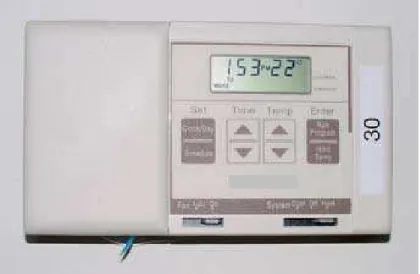
The programmable thermostat (pictured in Figure 2) controlled the house temperature. This particular thermostat offered a preset daytime setback from 9:00 to 16:00 Monday to Friday, and a daily nighttime setback from 23:00 to 6:00. These preset time periods were used for this project.

(15)

Figure 2 – Programmable Thermostat

2.3 Energy Consumption Measurements

Gas Consumption

Two modified gas meters with a pulse output connected to the main data acquisition system (DAS) monitored gas consumption of the furnace at a rate of 1 pulse per 0.05 ft3. The total gas consumption data was collected at 5-minute intervals.

Electrical Consumption

Two electric pulse-meters measured furnace and air conditioning electrical consumption at 1 pulse = 0.0006 kWh. This data was collected at 5-minute intervals by the DAS. Total daily furnace consumption and daily air-conditioning consumption were calculated from the 5-minute readings and this information was used in the analysis.

Furnace On-time Measurement

Furnace fan “on-time” was measured, indicating the total amount of time the furnace fan circulation motor ran at high speed (heating or cooling mode), as opposed to circulation speed. On-time data was collected by another data acquisition system in place to monitor transient performance of mechanical equipment at much shorter time intervals – 10 seconds. Total daily on-time was calculated from this data and was used in the analysis.

2.4 Temperature Measurements

In addition to the energy consumption measurements, the overall effect of thermostat setback on the house and occupants needs to be understood. During both summer and winter trials, house floor temperatures (basement, main floor, 2nd floor) were examined. Window and drywall surface temperatures were

(16)

examined during winter experiments only, in order to determine condensation risks.

It must be noted that temperature measurements were recorded hourly. They are an average of temperature measurements taken throughout the hour at 5 minute intervals. As a result, detailed information on short-term temperature fluctuations resulting in maximums (peaks) and minimums (valleys) are lost in the averaging process.

Five days were chosen for temperature analysis in each of the thermostat trials. Five consecutive days were not available in all cases. Days were instead chosen to include the coldest possible outdoor temperature in winter or the hottest possible outdoor temperature in summer: when temperature effects would be most prominent.

Table 4- Dates for House Temperature Analysis

Winter Trial Dates Minimum Outdoor Temperature Winter Benchmarking (22°C) Jan 10, 11, 12, 13, 15 -21.81°C

18°C Setback (day and night) Jan 6, 7, 17, 18, 19 -23.13°C

16°C Setback (day and night) Jan 25, 26, 27, 28, 29 -26.86°C

Summer Trial Dates Maximum Outdoor Temperature Summer Benchmarking (22°C) Jun 26, 27, 28, 29, 30 34.41°C

25°C Setforward (day) Aug 6, 7, 8, 9, 10 29.61°C

24°C Setting Jul 22, 23, 24, 25, 26 28.11°C

House Temperatures

Changes in basement, main floor and 2nd floor temperatures were tracked in both houses to help understand the overall effect of thermostat setback. These temperatures were measured at mid-wall height. The thermostat itself is located in the hallway of the main floor, beside the main floor thermocouple.

Drywall Surface Temperature

The main concern in examining drywall surface temperatures is to ensure that temperatures do not approach the dew point of surrounding air, leading to condensation problems.

The following graph shows the dew point temperatures for air and is referred to throughout the surface temperature analysis. Air at 22°C and 30% humidity will condense on a surface with a temperature below 3.7°C.

(17)

Dewpoint Temperature for air at 22°C, 18°C, and 16°C with varying humidity

-30.0 -20.0 -10.0 0.0 10.0 20.0 30.0 0 10 20 30 40 50 60 70 80 90 100 Relative humidity (%) D ew p oi n t Temperat u re (° C ) 22°C 18°C 16°C

Figure 3 - Dew point Temperature for 22°C, 18°C and 16°C air with varying humidity

(Source – derived from psychometric relationships published in ASHRAE Handbook of Fundamentals, ref 2)

Drywall surface temperatures were measured in the following locations:

• Living room – First Floor South facing • Nook – First Floor North facing • Dining room – First Floor West facing • Family room – First Floor East facing • Bedroom 2 – Second Floor South facing • Bedroom 2 – Second Floor West facing

Brick Air gap Sheathing Insulation Gypsum

Thermocouple Note: not to scale

(18)

Window Surface Temperature

Window temperature measurement is similarly important. If the window surface or frame temperature drops below the dew point of the ambient air, condensation (or ice) will form and may cause water damage to the surrounding wall. All windows in the CCHT houses are argon filled double-pane, with a low-E coating.

Window surface temperatures were measured at 5 different locations in each window (as shown in Figure 5). Three different windows were examined:

• Bedroom 2 – second floor south facing • Living room – first floor north facing • Dining room – first floor south facing

Indicates thermocouple location

Openable Window Centre of glass Edge of glass Edge of glass On frame On frame

Figure 5 - Thermocouple Location on Window Inner Surface

2.5 Recovery Time Calculation

The main floor thermocouple, located beside the thermostat, was used as the basis for recovery time calculations. The temperature of this thermocouple is captured at 5-minute intervals by the main data acquisition system. This gives a better resolution for calculating recovery time than other thermocouples in the house, whose temperatures are recorded hourly.

The benchmark condition was examined to determine the relationship between the daily average main floor temperature of the Reference house and the Test house. A graph outlining this relationship can be found in Appendix D.

(19)

temperature of the Test house for any given day during the setback and setforward trials. This “expected average” was set as the threshold temperature for determining recovery time. Recovery time was calculated from the point the thermostat automatically reset to 22°C to the time the house reached the threshold temperature. See Figure 24 for a sample graph showing recovery time.

2.6 Humidity Measurements

Humidity is an important factor in determining occupant comfort. During the winter setback experiments, the houses experienced very low humidity (around 10% RH) due to the fact that there were no real occupants, and no humidifiers were run.

In the summer, water is removed from the air in the form of condensation on the indoor air conditioner coil. During the summer trials, this condensation was collected and measured by means of a tipping scale with pulse output at a resolution of 0.011 L/pulse.

The relative humidity of each floor is recorded hourly by the main DAS. Relative humidity measurements in conjunction with hourly temperature measurements were used to calculate the humidity ratio of air (grams vapor per kg air) for each floor of the house. The three humidity ratios – for basement, main floor and 2nd floor – were then averaged to generate an average house humidity ratio. This allowed the moisture content of the Test and Reference House to be compared.

2.7 Weather Measurements

Outdoor temperature and humidity were measured and recorded every 5 minutes by means of a thermocouple and humidity sensor mounted on the exterior of the Reference House.

During the summer experiments, solar radiation incident on the south wall of the Reference House was measured on a 5-minute basis by a wall-mounted pyronometer. See Figure 6 for sample data. This data was then used to separate cloudy days from sunny days during the setforward experiment. A total vertical solar radiation of 8.5 MJ/m2/day was arbitrarily chosen to divide cloudy days from sunny days.

(20)

CCHT Research Houses Solar Energy 0.0 100.0 200.0 300.0 400.0 500.0 600.0 700.0 0:00:00 4:00:00 8:00:00 12:00:00 16:00:00 20:00:00 0:00:00 Time So la r En e rg y ( W /m ^ 2 ) 18-Jul-03

Figure 6 - Sample data from the CCHT Reference House Solar Pyranometer

Solar Data during Setforward Experiment

0 2000 4000 6000 8000 10000 12000 14000 16000 1 2 3 4 5 6 7 8 9 10 11 12 13 14 15 16 17 18 19 20 Day Inc id e nt V e rt ic a l S ol a r R a di a ti on (k J /m ^ 2 /da y ) sunny cloudy

Figure 7 - Division of Summer days by Measure of Incident Solar Radiation

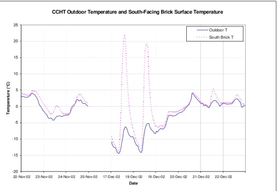
At the time of the winter setback experiment the pyronometer had not yet been installed. In order to see the effect of solar radiation on the thermostat experiment, the outer brick temperature of the south-facing wall of the Reference House was used to differentiate between sunny and cloudy days. On a sunny day, this

(21)

temperature can rise upwards of 20°C above the surrounding outdoor temperature. On a cloudy day, the brick temperature tracks the outdoor temperature within a few degrees. A threshold of 20°C difference between outdoor temperature and brick temperature was chosen arbitrarily to indicate sunny days, and less than a 5°C difference was chosen to indicate cloudy days.

See the following figures for a sample of brick temperature data. In this example, December 17th and 18th were classified as sunny days, and the rest were cloudy. In this way, the 18°C day and night setback data were separated into sunny, cloudy and mixed days (temperature difference between 5°C and 20°C). Not enough 16°C Day and Night Setback data were collected to separate in this manner.

It should be noted that because of the nature of the data, summer data was divided into two groups (sunny & cloudy), while winter data was divided into 3 groups (sunny, cloudy & mixed). Most winter days were either perfectly sunny or cloudy days, with only two days that could be classified as “mixed”. As a result, sunny and cloudy data formed two very distinct trends (both R2 values were larger than 0.995) with two days of “mixed” data clearly not belonging to either trend. In summer, there was more of a mix of weather with very few completely sunny days or completely cloudy days. This is shown in Figure 7, where only the 14th and 19th day on this graph could be said to be fully sunny. In essence, almost all days were “mixed”. For this reason, a threshold was chosen to split the “mixed” data into two trends with R-squared values of 0.993 (cloudy) and 0.989 (sunny). As expected by the mixed summer weather, resultant summer trends show more scatter than winter trends.

CCHT Outdoor Temperature and South-Facing Brick Surface Temperature

-20 -15 -10 -5 0 5 10 15 20 25

22-Nov-02 23-Nov-02 24-Nov-02 25-Nov-02 17-Dec-02 18-Dec-02 19-Dec-02 20-Dec-02 21-Dec-02 22-Dec-02

Date Te mpe ra tur e (° C ) Outdoor T South Brick T

(22)

Difference between South-Facing Brick Surface Temperature and Outdoor Temperature As an Indication of Solar Radiation

-5 0 5 10 15 20 25 30

22-Nov-02 23-Nov-02 24-Nov-02 25-Nov-02 17-Dec-02 18-Dec-02 19-Dec-02 20-Dec-02 21-Dec-02 22-Dec-02

Date and Time

de lt a Te m p e ra tur e ( °C )

delta T (Brick - Outdoor)

sunny

cloudy

Figure 9 - Difference between South-Facing Brick Surface Temperature and Outdoor Temperature as an Indication of Solar Radiation

(23)

3 Results

3.1 Benchmarking

3.1.1 Winter Benchmark

To compare the performance of the houses, daily consumption is plotted. Each point on the consumption graph represents a day with the Reference House value as the X-coordinate, and the Test House value as the Y-coordinate. If the benchmark were “perfect”, we would expect the data to form a linear trend with a slope of one and intercept of zero.

During the heating season, the mid-efficiency furnaces in the two houses performed very similarly in gas consumption (slope of 1.0437) and in on-time (slope of 1.0489). Unfortunately, differences in electrical consumption were apparent, emerging as a slope of 1.2044 on the electrical consumption graph. This is a result of differences in the power draw (Wattage) of the two motors in heating speed. These power differences are partially due to static pressure differences in the ducting causing different loads on the motors, as well as inherent differences in the motors themselves.

CCHT Research Houses - Winter 2002-2003 Benchmark Mid-Efficiency Furnace On Time (PSC motor)

y = 1.0489x - 17.339 R2 = 0.9972 0 144 288 432 576 720 0 144 288 432 576 720

Reference House Heating On Time (min)

T e s t H o u s e H e a tin g On T im e ( m in )

(24)

CCHT Research Houses - Winter 2002-2003 Benchmark Mid-Efficiency Furnace Electrical Consumption (PSC motor)

y = 1.2044x - 1.7886 R2 = 0.9961 8 9 10 11 12 8 9 10 11 12

Reference House Furnace Electrical Consumption, kWh/day

T e s t H o us e Fu rna c e E le c tr ic a l C ons u m pt ion , kW h /d a y

Figure 11 - Winter 2002-2003 Benchmark - Furnace Electrical Consumption

CCHT Research Houses - Winter 2002-2003 Benchmark Mid-efficiency Furnace Gas Consumption (PSC motor)

y = 1.0437x - 12.264 R2 = 0.9969 0 100 200 300 400 500 600 700 800 0 100 200 300 400 500 600 700 800

Reference House Gas Consumption, MJ/day

Te s t H o u s e G a s C ons ump ti o n, M J /d a y

(25)

3.1.2 Summer Benchmark

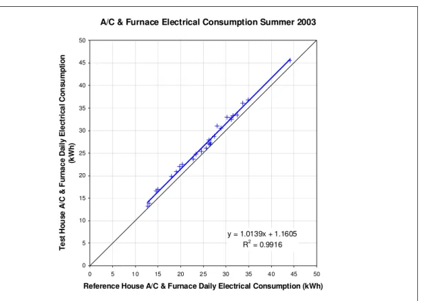
Similar trends are apparent in the summer benchmarking results. During the 2003 cooling season, the houses experienced similar on-times and air conditioner consumption, shown in the following graphs. However, differences in furnace fan motor performance resulted in higher Test House electrical consumption.

CCHT Research Houses - Benchmark Summer 2003 Air Conditioner On Time

y = 0.9552x + 51.667 R2 = 0.9888 0 144 288 432 576 720 864 1008 1152 1296 1440 0 144 288 432 576 720 864 1008 1152 1296 1440

Reference House AC On Time (min)

T e s t H o u s e A C On T im e ( m in )

(26)

CCHT Research Houses - Summer 2003 Benchmark Mid-Efficiency Furnace Electrical Consumption (PSC motor)

y = 1.2103x - 1.6069 R2 = 0.9912 8 9 10 11 12 13 14 8 9 10 11 12 13 14

Reference House Furnace Daily Electrical Consumption (kWh)

T e s t H o us e Fu rna c e D a il y E le c tr ic a l C o n s u m pt io n (k W h )

Figure 14 - Summer 2003 Benchmark - Furnace Electrical Consumption

CCHT Research Houses - Summer 2003 Benchmark Air Conditioner Electrical Consumption

y = 0.988x + 1.0781 R2 = 0.9914 0 5 10 15 20 25 30 35 40 0 5 10 15 20 25 30 35 40

Reference House A/C Daily Electrical Consumption (kWh)

Te s t H ou s e A /C D a il y E le c tr ic a l C ons u m pt ion ( k W h)

(27)

A/C & Furnace Electrical Consumption Summer 2003 y = 1.0139x + 1.1605 R2_{= 0.9916} 0 5 10 15 20 25 30 35 40 45 50 0 5 10 15 20 25 30 35 40 45 50

Reference House A/C & Furnace Daily Electrical Consumption (kWh)

T es t H o u s e A /C & F u rn ace D a il y E lec tr ic al C o n s u m p ti o n (k W h )

(28)

3.2 Winter Thermostat Experiment Results

3.2.1 Furnace On-Times

Furnace gas and electrical consumption are both closely related to furnace on-time. Trends in the on-time data are indicative of savings trends: the less the furnace runs in heating mode, the more the energy savings. The benchmark trend and thermostat data are plotted in Figure 17. The vertical drop from the benchmark line to the thermostat experiment trend lines indicates a reduction in on-time. As expected, thermostat setback data show that the introduction of a nighttime thermostat setback reduces furnace on-time. The following observations can be drawn from this data:

• Decrease in thermostat setback temperature results in a reduction in furnace on-time per day • Additional setback periods (daytime and nighttime) further reduce on-time

CCHT Research Houses - Thermostat Setback Experiment Mid-Efficiency Furnace On Time (PSC motor)

y = 1.0489x - 17.339 R2 = 0.9972 y = 0.7642x + 22.009 R2_{= 0.9754} y = 0.8816x + 5.6911 R2_{= 0.9922} y = 0.6797x + 39.3 R2 = 0.9928 0 144 288 432 576 720 0 144 288 432 576 720

T e s t H o u s e H e at in g On T im e ( m in ) Thermostat Setback 23:00 - 6:00 18°C Thermostat Setback 23:00 - 6:00 18°C 9:00 - 16:00 18°C Thermostat Setback 23:00 - 6:00 16°C 9:00 - 16:00 16°C Linear (Benchmark)

Linear (Thermostat Setback 23:00 -6:00 18°C 9:00 - 1-6:00 18°C)

Linear (Thermostat Setback 23:00 -6:00 18°C)

Figure 17 - Thermostat Setback Experiment - Furnace On-time

We can see from the different slopes of the setback data that as furnace on-time increases (to cope with cold weather conditions), the percentage of on-time savings increase. Therefore, we will find the greatest savings on the coldest day of the heating season. In this experiment, the coldest day of the season was

(29)

January 22nd 2003 (High -19°C, Low -27°C). On this day, the Reference House Furnace ran for 697 minutes. In benchmarking conditions we would expect the Test House furnace to run in heating mode for 714 minutes. Calculated maximum reduction in on-time for the Test House on this coldest day are summarized in the following table.

Table 5 - Maximum Calculated Reduction in On-time - from coldest day data Setting Calculated On-time*

(min) Calculated Reduction (min) Reduction (%) Winter Benchmark 714 --- --- 18°C nighttime setback 620 94 13

18°C day and nighttime setback 555 159 22

16°C day and nighttime setback 513 201 28

*Calculated by applying the on-time correlations (Figure 17) to the Reference House coldest day data (on-time of 697 minutes)

3.2.2 Electrical Consumption

The same trends can be seen in electrical savings. The more hours the house remains at the setback temperature, the lower the setback temperature, and the cooler the conditions outside, the greater the electrical savings.

CCHT Research Houses - Thermostat Setback Experiment Mid-Efficiency Furnace Electrical Consumption (PSC motor)

y = 1.2044x - 1.7886 R2 = 0.9961 y = 0.9956x + 0.1344 R2_{= 0.9903} y = 0.8967x + 0.9752 R2_{= 0.9725} y = 0.8124x + 1.7447 R2 = 0.997 8 9 10 11 12 8 9 10 11 12

Reference House Furnace Electrical Consumption, kWh/day Te s t H o u s e Fu rn a c e E le c tr ic a l C o n s u m pt io n , k W h/ da y Thermostat Setback 23:00 - 6:00 18°C Thermostat Setback 23:00 - 6:00 18°C 9:00 - 16:00 18°C Thermostat Setback 23:00 - 6:00 16°C 9:00 - 16:00 16°C

Linear (Benchmark Fall 2002)

(30)

On the coldest winter day this season, the Reference House furnace consumed 11.62 kWh of electricity. In benchmarking conditions we would expect the Test House furnace to consume 12.21 kWh. Calculated reductions in electrical consumption for the Test House in setback conditions on this coldest day are summarized in the following table.

Table 6 – Maximum Calculated Reduction in Electrical Consumption– from coldest day data Setting Calculated Consumption* (kWh/day) Calculated Reduction (kWh/day) Reduction (%) Winter Benchmark 12.208 --- --- 18°C nighttime setback 11.704 0.504 4.1

18°C day and nighttime setback 11.396 0.812 6.7

16°C day and nighttime setback 11.186 1.022 8.4

*Calculated by applying the electrical consumption correlations (Figure 18) to the Reference House coldest day data (electrical consumption of 11.62 kWh)

3.2.3 Gas Consumption

Gas data follow the same trends.

CCHT Research Houses - Thermostat Setback Experiment Mid-Efficiency Furnace Gas Consumption (PSC motor)

y = 1.0437x - 12.264 R2 = 0.9969 y = 0.8901x + 19.717 R2_{= 0.9932} y = 0.8158x + 31.62 R2_{= 0.9897} y = 0.7579x + 41.273 R2_{= 0.9989} 0 100 200 300 400 500 600 700 800 0 100 200 300 400 500 600 700 800

Reference House Gas Consumption, MJ/day

T e st H o u se G a s C o n s u m p ti o n , M J /d ay Thermostat Setback 23:00 - 6:00 18°C Thermostat Setback 23:00 - 6:00 18°C 9:00 - 16:00 18°C Thermostat Setback 23:00 - 6:00 16°C 9:00 - 16:00 16°C

Linear (benchmark fall 2002)

Figure 19 - Thermostat Setback Experiment - Furnace Gas Consumption

On the coldest day in the heating season (January 22nd 2003, High -19°C, Low -27°C), the Reference House Furnace consumed 759.1 MJ. In benchmarking conditions we would expect the Test House furnace

(31)

to consume 780.0 MJ. Calculated reductions in gas consumption for the Test House on this coldest day are summarized in the following table.

Table 7 - Maximum Calculated Reduction in Gas Consumption - from coldest day data Setting Calculated Consumption* (MJ/day) Calculated Reduction (MJ/day) Reduction (%) Winter Benchmark 780.0 --- --- 18°C nighttime setback 695.4 84.6 11

18°C day and nighttime setback 650.9 129.1 17

16°C day and nighttime setback 616.6 163.4 21

*Calculated by applying the gas consumption correlations (Figure 19) to the Reference House coldest day data (gas consumption of 759.1 MJ)

For projected savings over the entire heating season, please refer to Section 4.1.

3.2.4 Effect of Solar radiation on results

Splitting winter data into “cloudy” and “sunny” days highlights the effects of solar radiation on daytime setback savings.

On some sunny days, the added energy from solar radiation can keep the house from even reaching the setback temperature. This reduces the added savings of a daytime setback. Daytime setback is most effective on cloudy days.

Effect of Sunny days on 18°C Day & Night Thermostat setback On Time ( Mid-Efficiency Furance with PSC motor)

y = 0.7833x + 24.269 R2_{= 0.9986} y = 0.6777x + 50.062 R2_{= 0.9958} 216 288 360 432 504 576 648 216 288 360 432 504 576 648

Te s t H ou s e H e a ti n g O n Ti m e ( m in ) Sunny Mixed Cloudy Linear (Sunny) Linear (Cloudy) Linear (Benchmark) Thermostat Setback 23:00 - 6:00 18°C 9:00 - 16:00 18°C

(32)

Effect of Sunny days on 18°C Day & Night Thermostat setback Furnace Electrical Consumption ( Mid-Efficiency Furance with PSC Motor)

y = 0.9237x + 0.756 R2 = 0.9967 y = 0.796x + 1.9655 R2 = 0.9907 8 8.5 9 9.5 10 10.5 11 11.5 8 8.5 9 9.5 10 10.5 11 11.5

Reference House Furnace Elec Consumption, kWh/day

Te s t H ous e F ur na c e E le c C ons ump ti o n, k W h/ da y Sunny Mixed Cloudy Linear (Sunny) Linear (Cloudy) Linear (Benchmark) Thermostat Setback 23:00 - 6:00 18°C 9:00 - 16:00 18°C

Figure 21 - Effect of Sunny days on 18°C Day & Night Thermostat Setback Furnace Electrical Consumption

Effect of Sunny days on 18°C Day & Night Thermostat setback Gas Consumption ( Mid-Efficiency Furance with PSC motor)

y = 0.8206x + 36.001 R2 = 0.9966 y = 0.7636x + 47.955 R2 = 0.9938 0 100 200 300 400 500 600 700 0 100 200 300 400 500 600 700

Reference House Furnace Gas Consumption, MJ/day

T e st H o u s e F u rn ace Ga s C o n s u m p ti o n , MJ /d a y Sunny Mixed Cloudy Linear (Sunny) Linear (Cloudy) Linear (Benchmark) Thermostat Setback 23:00 - 6:00 18°C 9:00 - 16:00 18°C

Figure 22 - Effect of Sunny days on 18°C Day & Night Thermostat Setback Furnace Gas Consumption

(33)

3.2.5 Recovery Time

Perhaps one of the most important factors in examining thermostat setback is recovery time – the amount of time taken for the house air to return to its original temperature setting. Recovery time is a function of the minimum house temperature reached during the setback, irrespective of whether the setback is day or night. This relationship is shown in Figure 23. The circled data points on this graph indicate that the furnace ran more than once to reach the threshold temperature. An example of this phenomenon is shown in Figure 25. These points are included in the R2 value.

The lower the temperature the house is permitted to reach, the longer the recovery time. During the 18 °C setback, the main floor temperature of the Test House dropped to almost 16°C on the coldest winter days, requiring 1.5 hours to recover. At the 16°C setback setting, the house was allowed to drop to 14.5°C on the coldest days and required almost 2 hours of recovery time. Recovery time will directly affect the comfort of the occupants in the early morning hour and upon return from work. It can be expected that in less energy-efficient homes, recovery times may be longer.

Characteristics of the thermostat also come into play. The deadband is a temperature range around the setpoint used to control furnace operation. It is an important factor in the control of the house temperature, allowing the furnace to run for fewer and longer cycles. When the house cools down to the lower boundary of the deadband, heating is triggered. Once the house is heated up to the top of the deadband, the heating demand is satisfied and heating stops. The thermostat used for this experiment produced a measured average of ~21.5°C when set to 22°C, with a deadband of about 20.5°C to 22.5°C. A setting of 18°C produced a deadband of about 16.2°C to 18.2°C (see Figure 25).

This particular thermostat also has a feature called “anticipation” that is intended to prevent the house temperature from overshooting the setpoint. The anticipator, common to many programmable thermostats, comes into play during the recovery period, causing the furnace to cycle as it approaches the setpoint temperature (See Figure 27). Although anticipation improves overall temperature control, it may add significantly to recovery times from thermostat setback.

Cool surface temperatures may also be a factor in increasing recovery times. Air temperatures may temporarily reach thermostat settings, only to drop quickly because of lagging cool surfaces. More investigation of this phenomenon is needed to develop a better understanding.

(34)

CCHT Test House Minimum Main Floor Temperature VS Recovery time Thermostat Setback y = 0.0512x2 - 2.0708x + 21.01 R2 = 0.8689 0.0 0.5 1.0 1.5 2.0 2.5 13.5 14.5 15.5 16.5 17.5 18.5 19.5 20

Test House Minimum Main Floor T (°C)

Re c o v e ry T im e ( h o u rs ) .5 18 night

18 day & night - night 18 day & night - day 16 day & night - night 16 day & night - day 2 or more furnace runs to reach threshold T

Figure 23 - Thermostat Setback Recovery Time Winter 2002-2003

CCHT Research Houses Main Floor Temperature 18°C Night Setback (23:00 - 6:00) 12 13 14 15 16 17 18 19 20 21 22 23 24 25 26 18:00 20:00 22:00 0:00 2:00 4:00 6:00 8:00 10:00 12:00 14:00 16:00 Time T em p er at u re ( °C ) Reference House Test House

Threshold T emperature for Recovery 18-Dec-02

setback period

recovery period

Figure 24 - Sample Recovery Time for 18°C Night Setback 18-Dec-02 (outdoor temperature: -14.4°C min, -5.0°C max, sunny day)

(35)

CCHT Research Houses Main Floor Temperature 18°C Night Setback (23:00 - 6:00) 12 13 14 15 16 17 18 19 20 21 22 23 24 25 26 18:00 20:00 22:00 0:00 2:00 4:00 6:00 8:00 10:00 12:00 14:00 16:00 Time T em p er at u re ( °C ) Reference H ouse Test H ouse

Threshold T emperature for Recovery 22-Jan-03

setback period

recovery period

Figure 25 - Sample Recovery Time for 18°C Night Setback 22-Jan-03, showing 2 furnace runs to reach the threshold temperature for recovery (outdoor temperature: -27.5°C min, -19.2°C max)

CCHT Research Houses Main Floor Temperature 18°C Night Setback (23:00 - 6:00) 12 13 14 15 16 17 18 19 20 21 22 23 24 25 26 0:00 2:00 4:00 6:00 8:00 10:00 12:00 14:00 16:00 18:00 20:00 22:00 Time T em p er at u re ( °C ) Reference House Tes t House

Threshold Temperature for Recovery 03-Jan-03 night setback period 1st recovery period day setback period 2nd recovery period

Figure 26 - Sample Recovery Time for 18°C Night and Day Setback 03-Jan-03 (outdoor temperature: -8.5°C min, -4.7°C max)

(36)

CCHT Research Houses Main Floor Temperature 16°C Night Setback (23:00 - 6:00) 12 13 14 15 16 17 18 19 20 21 22 23 24 25 26 0:00 2:00 4:00 6:00 8:00 10:00 12:00 14:00 16:00 18:00 20:00 22:00 Time T em p er at u re ( °C ) Reference House Test House

Threshold Temperature for Rec overy 28-Jan-03 night setback period 1st recovery period day setback period 2nd recovery period

Figure 27 - Sample Recovery Time for 16°C Night and Day Setback (outdoor temperature: -27.0°C min, -14.6°C max)

3.2.6 House Temperatures

Benchmarking shows that the Test House temperature is maintained slightly above the Reference House temperature. This is likely due to small differences in the accuracy of the thermostats.

Except on sunny days, the main floor temperature in both houses remains above the second floor temperature, even throughout thermostat setback.

The effects of the setback are most prominent on the main floor: minimum temperatures follow thermostat settings closely. Differences in the second floor temperatures appear to be slightly smaller.

The most interesting effects are shown in the basement. The minimum temperatures in the two basements remain close throughout all trials, showing a 1.65°C difference during the 16°C setback (as opposed to the 5.34°C temperature difference on the main floor). Also, maximum basement temperatures are higher in the Test house than the Reference house during the setback days. This could be a result of the furnace running for an extended period of time whenever the thermostat returns to the 22°C setting, adding heat to the Test house basement. Mass effects of the concrete walls and slab, and mass of the equipment in the Test House Basement may be a contributing factor.

(37)

Table 8 - Minimum House Temperatures

Main Floor (°C) 2nd

Floor (°C) Basement (°C) Test Ref Difference Test Ref Difference Test Ref Difference 22°C Benchmark 21.69 21.27 0.42 20.01 19.57 0.44 16.68 17.02 -0.34

18°C Setback 18.06 21.1 -3.04 16.93 19.79 -2.86 14.26 15.72 -1.46

16°C Setback 15.81 21.15 -5.34 14.77 19.41 -4.64 13.67 15.32 -1.65

Table 9 - Maximum House Temperatures

Main Floor (°C) 2nd Floor (°C) Basement (°C) Test Ref Difference Test Ref Difference Test Ref Difference 22°C Benchmark 22.81 22.53 0.28 24.35 23.39 0.96 20.24 20.03 0.21

18°C Setback 22.56 22.36 0.2 23.14 23.46 -0.32 22.21 20.09 2.12

16°C Setback 22.72 22.48 0.24 22.75 23.35 -0.6 20.96 19.8 1.16

Detailed graphs of house temperatures can be found in Appendix A.

Drywall inner surface T

Table 10 - Minimum Drywall Surface Temperatures Measured on Centre of Insulated Stud Space

Test House Reference House Min T (°C) Location

RH resulting in condensation

Min T (°C) Location RH resulting in condensation 22°C Benchmarking 18.31 Bedroom 2 – West 80% @ 22°C 18.08 Bedroom 2 - South 79% @ 22°C

18°C Setback 14.88 Family room – East 64% @ 22°C 82% @ 18°C 17.83 Bedroom 2 - West 78% @ 22°C >100% @ 18°C

16°C Setback 12.74 Family room – East 55% @ 22°C 81% @ 16°C 17.80 Bedroom 2 - South 78% @ 22°C >100% @ 16°C

The coldest drywall surface temperature measured in the Test House during these trials was 12.74°C (during the 16°C Setback experiment). For the same experiment, the coldest drywall surface temperature in the Reference House was 17.80°C. In order for this to cause condensation problems in the test house, the humidity of the air at 22°C would have to exceed 55%. In the Reference House, air humidity would have to exceed 78%.

See Appendix B for detailed graphs of the drywall temperatures. The coldest drywall temperatures in the Test house occur for the most part in the morning. At this time we would expect a bedroom, having been occupied throughout the night, to have the highest humidity levels. During sunny days, drywall

(38)

It should be noted that these drywall surface temperatures were measured at the centre of an insulated wall cavity, and lower surface temperatures could be expected on the wall stud framing, at the bottom plates, at corners, or in sections with poorer thermal characteristics.

During the setback trials, drywall surface temperatures were seen to rise and fall in synch with air

temperature, while remaining approximately 2-degrees cooler – with the exception of sunny days, when the surface temperatures on south facing walls rose above the room air temperature (see Figure 28 to Figure 31). No distinct lag between wall and air recovery time was seen in the hourly data, a higher rate of data sampling could reveal a different result.

Drywal Inner Surface Temperatures in the Reference House (no setback) that were Concurrent with those in the Test House during the

18C Night and Day Setback Experiment

10 12 14 16 18 20 22 24 26 28 0:00 0:00 0:00 0:00 0:00 0:00 Time Te mpe ra tur e ( °C )

Livingroom drywall - South Nook drywall - North Main Floor Air T

06-Jan-03 07-Jan-03 17-Jan-03 18-Jan-03 19-Jan-03

Figure 28 - Reference House Air and Drywall Surface Temperature during the 18°C Night and Day Setback Experiment

(39)

Test House

18°C Night and day Setback - Drywall Inner Surface Temperatures

10 12 14 16 18 20 22 24 26 28 0:00 0:00 0:00 0:00 0:00 0:00 Time Te mpe ra tur e ( °C )

Main Floor air T Livingroom drywall - South Nook drywall - North

06-Jan-03 07-Jan-03 17-Jan-03 18-Jan-03 19-Jan-03

Figure 29 - Test House Air and Drywall Surface Temperature - 18°C Night and Day setback

Drywal Inner Surface Temperatures in the Reference House (no setback) that were Concurrent with those in the Test House during the

16°C Night and Day Setback Experiment

10 12 14 16 18 20 22 24 26 28 0:00:00 0:00:00 0:00:00 0:00:00 0:00:00 0:00:00 Time T em p e rat u re ( °C )

25-Jan- 26-Jan-03 27-Jan-03 28-Jan-03 29-Jan-03

Figure 30 - Reference House Air and Drywall Surface Temperature during the 16°C Night and Day setback experiment

(40)

Test House

16°C day and night setback - Drywall Inner Surface Temperatures

10 12 14 16 18 20 22 24 26 28 0:00:00 0:00:00 0:00:00 0:00:00 0:00:00 0:00:00 Time T em p er at u re ( °C )

25-Jan- 26-Jan-03 27-Jan-03 28-Jan-03 29-Jan-03

Figure 31 - Test House Air and Drywall Surface Temperature - 16°C Night and Day setback Window Surface Temperatures

The following tables present temperatures reached on the inner surface of the Test and Reference House windows (locations are shown in Figure 5). All windows in the house are equipped with interior Venetian blinds with 2.5 cm wide, white colored slats. During the setback experiments, all blinds were kept lowered with a horizontal (open) orientation.

Table 11 - Minimum Window Temperatures - Bedroom 2 (2nd Floor South Facing)

Test House Reference House Min T (°C) Location RH resulting in condensation Min T (°C) Location RH resulting in condensation 22°C Benchmarking 2.23 Frame of openable 27% @ 22°C 5.28 Edge of openable 34% @ 22°C 18°C Setback -1.24 Frame of openable 21% @ 22°C 27% @ 18°C 4.93 Edge of glass 33% @ 22°C 42% @ 18°C 16°C Setback -3.19 Frame of openable 18% @ 22°C 27% @ 16°C 3.95 Edge of glass 31% @ 22°C 45% @ 16°C

(41)

Table 12 - Minimum Window Temperatures – Dining room (1st Floor North Facing)

Test House Reference House Min T (°C) Location RH resulting in condensation Min T (°C) Location RH resulting in condensation 22°C

Benchmarking 1.81 Edge of glass 26% @ 22°C 4.31 Edge of glass 31% @ 22°C 18°C Setback -1.43 Edge of glass 21% @ 22°C _{27% @ 18°C} 3.22 _openableFrame of 29% @ 22°C _{37% @ 18°C}

16°C Setback -4.99 Edge of glass 16% @ 22°C

23% @ 16°C -0.49

Frame of openable

22% @ 22°C 33% @ 16°C

Table 13 - Minimum Window Temperatures - Living room (1st Floor South Facing)

Test House Reference House Min T (°C) Location RH resulting in condensation Min T (°C) Location RH resulting in condensation 22°C Benchmarking -2.65 Frame of openable 19 % @ 22°C 1.02 Frame of openable 25% @ 22°C 18°C Setback -4.92 Frame of openable 16% @ 22°C 21% @ 18°C 0.10 Frame of openable 23% @ 22°C 34% @ 18°C 16°C Setback -7.81 Frame of openable 13% @ 22°C 19% @ 16°C -0.94 Frame of openable 22% @ 22°C 32% @ 16°C

For the most part, the lowest temperatures on the interior of the window occurred at the edge of the glass or the frame. This is an expected result and is consistent with lab assessments of surface temperatures of such windows4.

In the benchmarking phase, the Test and Reference House windows showed more variation than the drywall. For all three windows, the lowest benchmark temperatures measured in the Test House were approximately 3 degrees lower than the Reference House minimums. In both houses, the first floor Living room window reached the lowest temperatures. In the Reference House, condensation is predicted to occur with an RH above 22%. In the Test House, results from the 16-degree setback predict that condensation and ice would occur at a relative humidity above 13% @ 22°C (19% @ 16°C).

(42)

3.3 Summer Thermostat Experiment Results

3.3.1 Air Conditioner On-Time

On-time data is a measure of the amount of time the furnace circulation fan runs in high-speed cooling mode. Figure 32 shows that as Reference House furnace on-time increases, the vertical distance between the benchmark and setforward trend lines increases. This is an indication of increasing reductions in furnace on-time as more time is spent in cooling mode. On hotter, sunnier days, the furnace ran in cooling mode for the longest time, causing the largest reductions in AC on-time due to thermostat setforward. The spread of this data was due to solar gains (sunny VS cloudy days) as discussed in section 3.4.3.

The benefits gained from the setforward, as the house drifts to the higher temperature, is partially offset by the time the AC unit has to run to re-cool the house at the end of the setforward period. By contrast, we see larger reductions in AC on-time throughout the test period for the higher temperature setting, in Figure 32 the higher temperature correlation remains almost parallel to the benchmarking line. This setting produces an almost constant on-time reduction (~200 minutes), irrespective of outdoor temperature or solar gains.

CCHT Research Houses - Thermostat Setting Experiments Summer 2003 Air Conditioner On Time

y = 0.8042x + 44.557 R2 = 0.962 y = 0.8906x - 110.87 R2 = 0.9947 y = 0.9552x + 51.667 R2 = 0.9888 0 144 288 432 576 720 864 1008 1152 1296 1440 0 144 288 432 576 720 864 1008 1152 1296 1440

Reference House AC On Time (min)

Te s t H ou s e A C O n Ti m e ( m in) SetForward to 25°C 9:00 -16:00

Higher Temperature Setting (24°C)

Linear (Set-Forward)

Linear (Higher Temperature)

Linear (Benchmark)

Figure 32 - Summer Thermostat Experiments - Air Conditioner On-Time

We will find the greatest on-time reductions on the hottest day of the heating season. In this experiment, the hottest day of the season was June 26th 2003 (High 34.7°C, Low 23.2°C). On this day the Reference

(43)

House air conditioning ran for 1136 minutes. In benchmarking conditions we would expect the Test House air conditioning to run for 1137 minutes. Calculated maximum reductions in on-time for the Test House on this hottest day are summarized in the following table.

Table 14 - Maximum Calculated Reduction in On-time - from Hottest Day Data Setting Calculated On-time*

(min) Predicted Reduction (min) Reduction (%) 22°C Summer Benchmark 1137 --- --- 25°C Daytime Setforward 958 179 16

24°C Higher Temperature Setting 901 236 21

*Calculated by applying the on-time correlations (Figure 32) to the Reference House coldest day data (on-time of 1136 min)

3.3.2 Electrical Consumption

The same on-time trends are reflected directly in electrical consumption. Longer on-times result in higher electrical consumption, and higher electrical savings. On the hottest day, this translates into the following reductions:

Table 15 - Maximum Calculated Reductions in Air Conditioner Electrical Consumption - from Hottest Day Data

Setting Calculated Consumption* (kWh/day) Calculated Reduction (kWh/day) Reduction (%) 22°C Summer Benchmark 32.249 25°C Daytime Setforward 26.655 5.593 17

24°C Higher Temperature Setting 25.859 6.390 20

*Calculated by applying the AC electrical consumption correlations (Figure 33) to the Reference House coldest day data (AC electrical consumption of 31.549 kWh)

Table 16 - Maximum Calculated Reductions in Furnace Fan Electrical Consumption - from Hottest Day Data Setting Calculated Consumption* (kWh/day) Calculated Reduction (kWh/day) Reduction (%) 22°C Summer Benchmark 13.565 25°C Daytime Setforward 12.843 0.722 5.3

24°C Higher Temperature Setting 12.383 1.182 8.7

*Calculated by applying the furnace fan electrical consumption correlations (Figure 33) to the Reference House coldest day data (furnace fan electrical consumption of 12.536 kWh)

Table 17 - Maximum Predicted Reductions in A/C and Furnace Fan Electrical Consumption - from Hottest Day Data

Setting Calculated Consumption (kWh/day) Calculated Reduction (kWh/day) Reduction (%) 22°C Summer Benchmark 45.814 25°C Daytime Setforward 39.498 6.316 14

24°C Higher Temperature Setting 38.242 7.572 17