HAL Id: hal-00813409
https://hal.inria.fr/hal-00813409v2
Submitted on 25 Apr 2013
HAL is a multi-disciplinary open access
archive for the deposit and dissemination of
sci-entific research documents, whether they are
pub-lished or not. The documents may come from
teaching and research institutions in France or
abroad, or from public or private research centers.
L’archive ouverte pluridisciplinaire HAL, est
destinée au dépôt et à la diffusion de documents
scientifiques de niveau recherche, publiés ou non,
émanant des établissements d’enseignement et de
recherche français ou étrangers, des laboratoires
publics ou privés.
Blind Sensor Calibration in Sparse Recovery Using
Convex Optimization
Cagdas Bilen, Gilles Puy, Rémi Gribonval, Laurent Daudet
To cite this version:
Cagdas Bilen, Gilles Puy, Rémi Gribonval, Laurent Daudet. Blind Sensor Calibration in Sparse
Recovery Using Convex Optimization. SAMPTA - 10th International Conference on Sampling Theory
and Applications - 2013, Jul 2013, Bremen, Germany. �hal-00813409v2�
Blind Sensor Calibration in Sparse Recovery Using
Convex Optimization
C
¸ a ˘gdas¸ Bilen
∗, Gilles Puy
†, R´emi Gribonval
∗and Laurent Daudet
‡∗ INRIA, Centre Inria Rennes - Bretagne Atlantique, 35042 Rennes Cedex, France.
† Institute of Electrical Engineering, Ecole Polytechnique Federale de Lausanne (EPFL), CH-1015 Lausanne, Switzerland
‡Institut Langevin, CNRS UMR 7587, UPMC, Univ. Paris Diderot, ESPCI, 75005 Paris, France
Abstract—We investigate a compressive sensing system in which the sensors introduce a distortion to the measurements in the form of unknown gains. We focus on blind calibration, using measures performed on a few unknown (but sparse) signals. We extend our earlier study on real positive gains to two generalized cases (signed real-valued gains; complex-valued gains), and show that the recovery of unknown gains together with the sparse signals is possible in a wide variety of scenarios. The simultaneous recovery of the gains and the sparse signals is formulated as a convex optimization problem which can be solved easily using off-the-shelf algorithms. Numerical simulations demonstrate that the proposed approach is effective provided that sufficiently many (unknown, but sparse) calibrating signals are provided, especially when the sign or phase of the unknown gains are not completely random.
I. INTRODUCTION
Compressed sensing theory shows thatK-sparse signals can
be sampled at much lower rate than required by the
Nyquist-Shannon theorem [1]. More precisely, if x ∈ CN is a
K-sparse source vector then it can be captured by collecting only M ≪ N linear measurements
yi= m′ix, i = 1, . . . , M (1)
In the above equation, m1, . . . , mM ∈ CN are known
mea-surement vectors, and .′ denotes the conjugate transpose
op-erator. Under certain conditions on the measurement vectors, the signal can be accurately reconstructed by solving, e.g.,
x∗ℓ1= arg min z
kzk1
subject to yi= m′iz, i = 1, . . . , M
where k·k1 denotes the ℓ1-norm, which favors the selection
of sparse signals among the ones satisfying the measurement constraints. It has been shown that the number of measure-ments needed for accurate recovery of x scales only linearly
with K [1]. Note that the above minimization problem can
easily be modified to handle the presence of additive noise on the measurements.
Unfortunately, in some practical situations, it is some-times not possible to perfectly know the measurement vectors
m1, . . . , mM. In many applications dealing with distributed
This work was partly funded by the Agence Nationale de la Recherche (ANR), project ECHANGE (ANR-08-EMER-006) and by the European Research Council, PLEASE project (ERC-StG-2011-277906). LD is on a joint affiliation between Univ. Paris Diderot and Institut Universitaire de France.
sensors or radars, the location or intrinsic parameters of the sensors are not exactly known, which in turn results in unknown phase shifts and/or gains at each sensor [2], [3]. Similarly, applications with microphone arrays are shown to require calibration of each microphone to account for the unknown gain and phase shifts introduced [4]. Unlike additive perturbations in the measurement matrix, this multiplicative perturbation may introduce significant distortion if ignored [5], [6].
In this paper, we investigate the problem of estimating the unknown gains introduced by the sensors when multiple unknown but sparse input signals are measured. We extend the convex optimization approach dealing with positive real gains proposed in [7] to the case of signed real-valued and complex-valued gains which is more realistic from the application perspective. In addition to identifying the additional challenges introduced by the more difficult problem, we further demon-strate the performance of the proposed algorithms in cases where the unknown phase shifts (or sign changes) introduced by the sensors are not completely random.
II. PROBLEMDEFINITION
Suppose that the measurement system in (1) is perturbed by
complex gains at each sensor i and there are multiple sparse
input signals, xl ∈ CN, l = 1 . . . L, applied to the system
such that
yi,l= diejθimi′xl i = 1 . . . M, θi ∈ [0, 2π), di∈ R+
(2)
For a real valued system, the phase term ejθi
is replaced by
∓1 (or θi∈ {0, π}). We focus only on the noiseless case for
the sake of simplicity.
It should be noted that, unlike the case with positive real gains, ignoring the unknown gains during recovery is not a viable option when dealing with signed real or complex gains even when the magnitude of the gains are constant. This is due to the significant distortion introduced by the change in sign (and phase). Therefore it is essential to employ a reconstruction approach that deals with the unknown gains.
In a traditional recovery strategy, one can enforce the sparsity of the input signals while enforcing the measurement constraints in (2). However, when dealing with unknown gains, the measurement constraints are non-linear with respect to
with by using an alternate minimization strategy where one
iteratively estimates x while keeping di fixed and vice-versa
[2]. However, the convergence of this alternating optimization to the global minimum is not guaranteed since there is a chance that the algorithm gets stuck in a local minimum.
A. Proposed Approach
The recovery of xl, l = 1 . . . L and di, i = 1 . . . M with
convex optimization whenejθi
are known has been studied in [7]. In this paper, we extend the same approach to systems with signed real-valued and complex-valued gains. Therefore
the termdiejθi will henceforth simply be represented asdi ∈
R for real-valued systems and di ∈ C for complex-valued
systems.
As an alternative to the alternating non-linear optimization described above, the measurement equation (2) can be reorga-nized in a bi-linear fashion such that
yi,lτi= m′ixl i = 1 . . . M , l = 1 . . . L (3)
τi,
1 di
assuming that di 6= 0 ∀i. Consequently, one can attempt
to recover the sparse signals and the gains with the convex optimization x∗1, . . . , x∗L τ∗ 1, . . . , τM∗ = arg min z1,...,zL t1,...,tM L X n=1 kznk1 (4) subject to yi,lti= m′izl l = 1, . . . , L i = 1, . . . , M M X n=1 tn= c
for an arbitrary constant c > 0. The actual gains can be set
as d∗ i =
1 τ∗
i after the optimization. Note that even though the
minimized objective function is equivalent to the alternating non-linear optimization, the problems with local minimums are now eliminated thanks to the convexity of the formulation.
We can make several observations regarding the optimiza-tion in (4):
1) The constraint Pntn = c ensures that the trivial
solution (τi = 0, xl = 0, ∀i, l) is excluded from the
solution set.
2) The constraint Pntn = c also excludes the solutions
where the sum of the gains are zero. When dealing with signed real or complex valued gains, this may result in excluding the actual solution in rare cases where the sought out gains actually sum up to zero. How-ever, the probability of encountering this phenomena in real applications is often infinitesimally small. For the applications in which this possibility is higher, an alternative approach to deal with this case is discussed in Section III.
3) The measurement constraints are satisfied up to a global scale factor (and phase shift for complex signals),
there-fore the constantc can be set arbitrarily. Unfortunately,
the global scale (and phase) factor cannot be determined with the given optimization approach, although this is often not an issue in practical systems.
4) The successful recovery of the gains and the signals re-quire availability of more than one input signal (L > 1). Although this may seem like a restriction, acquiring data from multiple sources is often straightforward in many application fields.
III. EXPERIMENTALRESULTS
In order to test the performance of the proposed algorithm, phase transition curves as in the compressed sensing recovery
are plotted for a signal size N = 100 with the measurement
vectors, mi, and all the non zero entries in the input signals,
xl, randomly generated from an i.i.d. normal distribution. The
positions of the non-zero coefficients of the input signals, xl,
are chosen uniformly at random in{1, . . . , N }. The magnitude
of the gains were generated using |di| ∼ exp(N (0, σ2)),
where σ is the parameter governing the amplitude of
decal-ibration. For real valued experiments, the sign of the gains
are randomly assigned such that the probability,pr, of setting
a negative gain is adjusted to be pr ∈ {0, 0.16, 0.33, 0.5}.
Similarly for complex valued gains, the phase of the gains are
chosen uniformly at random from the range[0, 2πpc) where
pc ∈ {0, 0.33, 0.66, 1}. Note that the parameters pr and pc
determine the scale of ambiguity in the signs and phases where
maximum possible ambiguity is observed whenpr= 0.5 and
pc= 1 respectively.
The signals (and the gains) are recovered for different amount of decalibration amplitude (σ = 0.1, 0.3, 1) with sufficiently high number of input signals (L = 5, 10, 20 respectively). The proposed optimization in (4) is performed using an ADMM [9] based algorithm. The perfect
reconstruc-tion criteria is selected as L1 Plµ(xl, x∗l) > 0.9999, where
the absolute correlation factor µ(·, ·) is defined as
µ(x1, x2), |x
′ 1x2|
kx1k2kx2k2
(5) so that the global phase and scale difference between the source and recovered signals is ignored.
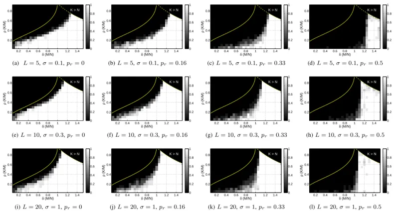
The probability of recovery (computed through 10 indepen-dent simulations for each set of parameters) of the proposed
method with respect to δ , M/N and ρ , K/M are
shown in Figures 1 and 2 for real valued and complex valued systems respectively. The first thing to notice from the results
is that the performance for pr = 0 (or pc = 0) is consistent
with the results presented in [7] as expected. The effect of increasing sign (or phase) ambiguity can be observed in the
results as pr (orpc) increases. Although the performance is
acceptable for pr as high as 0.33 (pc up to 0.66), there is a
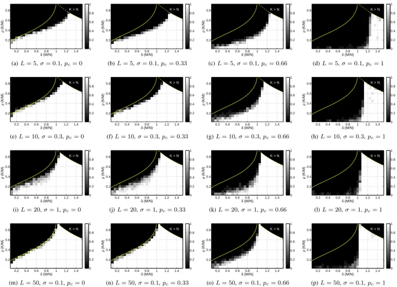
significant degradation when dealing very high sign (or phase) ambiguity such that signal recovery is impossible regardless of the sparsity, unless the measurement system is overcomplete (M > N ). This phenomena can best be observed in the last row of complex-valued results, Figures 2(m)-2(p), where the number of input signals is very large (L = 50) with respect to
δ (M/N) ρ (K/M) K > N 0.2 0.4 0.6 0.8 1 1.2 1.4 0.2 0.4 0.6 0.8 0 0.2 0.4 0.6 0.8 1 (a) L = 5, σ = 0.1, pr= 0 δ (M/N) ρ (K/M) K > N 0.2 0.4 0.6 0.8 1 1.2 1.4 0.2 0.4 0.6 0.8 0 0.2 0.4 0.6 0.8 1 (b) L = 5, σ = 0.1, pr= 0.16 δ (M/N) ρ (K/M) K > N 0.2 0.4 0.6 0.8 1 1.2 1.4 0.2 0.4 0.6 0.8 0 0.2 0.4 0.6 0.8 1 (c) L = 5, σ = 0.1, pr= 0.33 δ (M/N) ρ (K/M) K > N 0.2 0.4 0.6 0.8 1 1.2 1.4 0.2 0.4 0.6 0.8 0 0.2 0.4 0.6 0.8 1 (d) L = 5, σ = 0.1, pr= 0.5 δ (M/N) ρ (K/M) K > N 0.2 0.4 0.6 0.8 1 1.2 1.4 0.2 0.4 0.6 0.8 0 0.2 0.4 0.6 0.8 1 (e) L = 10, σ = 0.3, pr= 0 δ (M/N) ρ (K/M) K > N 0.2 0.4 0.6 0.8 1 1.2 1.4 0.2 0.4 0.6 0.8 0 0.2 0.4 0.6 0.8 1 (f) L = 10, σ = 0.3, pr= 0.16 δ (M/N) ρ (K/M) K > N 0.2 0.4 0.6 0.8 1 1.2 1.4 0.2 0.4 0.6 0.8 0 0.2 0.4 0.6 0.8 1 (g) L = 10, σ = 0.3, pr= 0.33 δ (M/N) ρ (K/M) K > N 0.2 0.4 0.6 0.8 1 1.2 1.4 0.2 0.4 0.6 0.8 0 0.2 0.4 0.6 0.8 1 (h) L = 10, σ = 0.3, pr= 0.5 δ (M/N) ρ (K/M) K > N 0.2 0.4 0.6 0.8 1 1.2 1.4 0.2 0.4 0.6 0.8 0 0.2 0.4 0.6 0.8 1 (i) L = 20, σ = 1, pr= 0 δ (M/N) ρ (K/M) K > N 0.2 0.4 0.6 0.8 1 1.2 1.4 0.2 0.4 0.6 0.8 0 0.2 0.4 0.6 0.8 1 (j) L = 20, σ = 1, pr= 0.16 δ (M/N) ρ (K/M) K > N 0.2 0.4 0.6 0.8 1 1.2 1.4 0.2 0.4 0.6 0.8 0 0.2 0.4 0.6 0.8 1 (k) L = 20, σ = 1, pr= 0.33 δ (M/N) ρ (K/M) K > N 0.2 0.4 0.6 0.8 1 1.2 1.4 0.2 0.4 0.6 0.8 0 0.2 0.4 0.6 0.8 1 (l) L = 20, σ = 1, pr= 0.5
Fig. 1: The probability of perfect recovery in the real valued system forN = 100 with respect to δ, M/N and ρ , K/M.
The solid yellow line indicates the Donoho-Tanner phase transition curve for fully calibrated compressed sensing recovery
[8]. The dashed yellow line indicates the boundary to the region whereK > N . Each row of figures display the change in
recovery performance with increasing sign ambiguity from left to right for a fixed set ofL and σ.
the variance in the gain magnitudes (σ = 0.1). The degradation in the results can be attributed to the significant increase in the contamination of the information in the measurements as the sign or phase ambiguity increases. Therefore recovery becomes possible only when there are sufficient number of measurements to overcome the high distortion. For the
maxi-mally ambiguous case (pr= 0.5, pc= 1), this is only possible
forM > N . Even though this is a drawback of the presented
approach, it should be noted that in many practical systems the sign (or phase) ambiguity is often not as severe as fully random, but within a limited range. Therefore the presented algorithm can still be applied in various scenarios.
As an alternative to the proposed method in this paper, a phase calibration algorithm (in which gain magnitudes are assumed to be known) that can recover the sparse signals along
with the unknown phases distributed within the entire[0, 2π)
range has been presented in [10], [11]. This approach for phase calibration can be combined with the proposed method in this paper in order to recover signed real-valued or complex-valued gains with maximum sign and phase ambiguity. It is also possible to use this combined approach for signal recovery in applications where the sum of the gains are likely to be zero.
IV. CONCLUSIONS ANDFUTUREWORK
In this paper, we have investigated the problem of estimating the unknown gains at each measurement sensor along with sparse input signals in a compressed sensing measurement system. We have extended the use of convex recovery strategy suggested for positive real gains to the more general cases of signed real-valued and complex-valued gains, and demon-strated the change of recovery performance with increasing sign and phase ambiguity.
The performance of the proposed algorithm is shown to be approaching to that of the unperturbed compressed sensing recovery when there are sufficient number sparse input signals unless the distribution of the sign changes or the phase shifts are maximally varying among the sensors. This drawback of the proposed algorithm can still be ignored for many application fields in which the ambiguity in the sign changes or the phase shifts at the sensors are within a limited range. For other applications, it is possible to combine the proposed method with other approaches employed for phase calibration to improve the recovery performance which is considered as a future work. The theoretical justification of the limitation of the proposed method for maximum sign and phase ambiguity is also a work in progress.
δ (M/N) ρ (K/M) K > N 0.2 0.4 0.6 0.8 1 1.2 1.4 0.2 0.4 0.6 0.8 0 0.2 0.4 0.6 0.8 1 (a) L = 5, σ = 0.1, pc= 0 δ (M/N) ρ (K/M) K > N 0.2 0.4 0.6 0.8 1 1.2 1.4 0.2 0.4 0.6 0.8 0 0.2 0.4 0.6 0.8 1 (b) L = 5, σ = 0.1, pc= 0.33 δ (M/N) ρ (K/M) K > N 0.2 0.4 0.6 0.8 1 1.2 1.4 0.2 0.4 0.6 0.8 0 0.2 0.4 0.6 0.8 1 (c) L = 5, σ = 0.1, pc= 0.66 δ (M/N) ρ (K/M) K > N 0.2 0.4 0.6 0.8 1 1.2 1.4 0.2 0.4 0.6 0.8 0 0.2 0.4 0.6 0.8 1 (d) L = 5, σ = 0.1, pc= 1 δ (M/N) ρ (K/M) K > N 0.2 0.4 0.6 0.8 1 1.2 1.4 0.2 0.4 0.6 0.8 0 0.2 0.4 0.6 0.8 1 (e) L = 10, σ = 0.3, pc= 0 δ (M/N) ρ (K/M) K > N 0.2 0.4 0.6 0.8 1 1.2 1.4 0.2 0.4 0.6 0.8 0 0.2 0.4 0.6 0.8 1 (f) L = 10, σ = 0.3, pc= 0.33 δ (M/N) ρ (K/M) K > N 0.2 0.4 0.6 0.8 1 1.2 1.4 0.2 0.4 0.6 0.8 0 0.2 0.4 0.6 0.8 1 (g) L = 10, σ = 0.3, pc= 0.66 δ (M/N) ρ (K/M) K > N 0.2 0.4 0.6 0.8 1 1.2 1.4 0.2 0.4 0.6 0.8 0 0.2 0.4 0.6 0.8 1 (h) L = 10, σ = 0.3, pc= 1 δ (M/N) ρ (K/M) K > N 0.2 0.4 0.6 0.8 1 1.2 1.4 0.2 0.4 0.6 0.8 0 0.2 0.4 0.6 0.8 1 (i) L = 20, σ = 1, pc= 0 δ (M/N) ρ (K/M) K > N 0.2 0.4 0.6 0.8 1 1.2 1.4 0.2 0.4 0.6 0.8 0 0.2 0.4 0.6 0.8 1 (j) L = 20, σ = 1, pc= 0.33 δ (M/N) ρ (K/M) K > N 0.2 0.4 0.6 0.8 1 1.2 1.4 0.2 0.4 0.6 0.8 0 0.2 0.4 0.6 0.8 1 (k) L = 20, σ = 1, pc= 0.66 δ (M/N) ρ (K/M) K > N 0.2 0.4 0.6 0.8 1 1.2 1.4 0.2 0.4 0.6 0.8 0 0.2 0.4 0.6 0.8 1 (l) L = 20, σ = 1, pc= 1 δ (M/N) ρ (K/M) K > N 0.2 0.4 0.6 0.8 1 1.2 1.4 0.2 0.4 0.6 0.8 0 0.2 0.4 0.6 0.8 1 (m) L = 50, σ = 0.1, pc= 0 δ (M/N) ρ (K/M) K > N 0.2 0.4 0.6 0.8 1 1.2 1.4 0.2 0.4 0.6 0.8 0 0.2 0.4 0.6 0.8 1 (n) L = 50, σ = 0.1, pc= 0.33 δ (M/N) ρ (K/M) K > N 0.2 0.4 0.6 0.8 1 1.2 1.4 0.2 0.4 0.6 0.8 0 0.2 0.4 0.6 0.8 1 (o) L = 50, σ = 0.1, pc= 0.66 δ (M/N) ρ (K/M) K > N 0.2 0.4 0.6 0.8 1 1.2 1.4 0.2 0.4 0.6 0.8 0 0.2 0.4 0.6 0.8 1 (p) L = 50, σ = 0.1, pc= 1
Fig. 2: The probability of perfect recovery in the complex valued system forN = 100 with respect to δ, M/N and ρ , K/M.
The solid yellow line indicates the Donoho-Tanner phase transition curve for fully calibrated compressed sensing recovery [8].
The dashed yellow line indicates the boundary to the region whereK > N . Each row of figures display the change in recovery
performance with increasing phase ambiguity from left to right for a fixed set ofL and σ. The last row, (m)-(p) shows the
performance limit for very highL.
REFERENCES
[1] David L. Donoho, “Compressed Sensing,” IEEE Transactions on
Information Theory, vol. 52, no. 4, pp. 1289 – 1306, 2006.
[2] Zai Yang, Cishen Zhang, and Lihua Xie, “Robustly stable signal
recovery in compressed sensing with structured matrix perturbation,” Signal Processing, IEEE Transactions on, vol. 60, no. 9, pp. 4658 – 4671, sept. 2012.
[3] Boon Chong Ng and Chong Meng Samson See, “Sensor-array calibra-tion using a maximum-likelihood approach,” Antennas and Propagacalibra-tion, IEEE Transactions on, vol. 44, no. 6, pp. 827 –835, jun 1996. [4] R. Mignot, L. Daudet, and F. Ollivier, “Compressed sensing for acoustic
response reconstruction: Interpolation of the early part,” in Applications of Signal Processing to Audio and Acoustics (WASPAA), 2011 IEEE Workshop on, oct. 2011, pp. 225 –228.
[5] Emmanuel J. Cands, Justin K. Romberg, and Terence Tao, “Stable signal recovery from incomplete and inaccurate measurements,” Communica-tions on Pure and Applied Mathematics, vol. 59, no. 8, pp. 1207–1223, 2006.
[6] M.A. Herman and T. Strohmer, “General deviants: An analysis of per-turbations in compressed sensing,” Selected Topics in Signal Processing, IEEE Journal of, vol. 4, no. 2, pp. 342 –349, april 2010.
[7] R´emi Gribonval, Gilles Chardon, and Laurent Daudet, “Blind calibration for compressed sensing by convex optimization,” in Acoustics Speech and Signal Processing (ICASSP), 2012 IEEE International Conference on, 2012, pp. 2713–2716.
[8] David L. Donoho and Jared Tanner, “Observed universality of phase transitions in high-dimensional geometry, with implications for modern data analysis and signal processing.,” Philosophical transactions. Series A, Mathematical, physical, and engineering sciences, vol. 367, no. 1906, pp. 4273–93, Nov. 2009.
[9] Stephen Boyd, Neal Parikh, Eric Chu, B Peleato, and Jonathan Eckstein, “Distributed optimization and statistical learning via the alternating direction method of multipliers,” Foundations and Trends in Machine Learning, vol. 3, no. 1, pp. 1–122, 2011.
[10] Cagdas Bilen, Gilles Puy, R´emi Gribonval, and Laurent Daudet, “Blind Sensor Calibration in Sparse Recovery,” in International Biomedical and Astronomical Signal Processing (BASP) Frontiers Workshop, Villars-sur-Ollon, Switzerland, Jan. 2013.
[11] Cagdas Bilen, Gilles Puy, R´emi Gribonval, and Laurent Daudet, “Blind Phase Calibration in Sparse Recovery,” in European Signal Processing Conference (EUSIPCO) (submitted), 2013.