1422-6928/07/030295-48 c
° 2006 Birkh¨auser Verlag, Basel DOI 10.1007/s00021-005-0200-8
Fluid Mechanics
Downstream Asymptotics in Exterior Domains:
from Stationary Wakes to Time Periodic Flows
Guillaume van BaalenCommunicated by G. P. Galdi
Abstract. In this paper, we consider the time-dependent Navier–Stokes equations in the half-space [x0, ∞) × R ⊂ R2, with boundary data on the line x = x0assumed to be time-periodic (or
stationary) with a fixed asymptotic velocity u∞ = (1, 0) at infinity. We show that there exist
(locally) unique solutions for all data satisfying a center-stable manifold compatibility condition in a certain class of functions. Furthermore, we prove that as x → ∞, the vorticity decomposes itself in a dominant stationary part on the parabolic scale y ∼√x and corrections of order x−3
2+ε, while the velocity field decomposes itself in a dominant stationary part in form of an explicit multi-scale expansion on the scales y ∼√x and y ∼ x and corrections decaying at least like x−9
8+ε. The asymptotic fields are made of linear combinations of universal functions with coefficients depending mildly on the boundary data. The asymptotic expansion for the component parallel to u∞ contains ‘non-trivial’ terms in the parabolic scale with amplitude
ln(x)x−1 and x−1. To first order, our results also imply that time-periodic wakes behave like
stationary ones as x → ∞.
The class of functions used to prove these results is ‘natural’ in the sense that the well known ‘Physically Reasonable’ (in the sense of Finn & Smith) stationary solutions of the Navier–Stokes equations around an obstacle fall into that class if the half-space extends in the downstream direction and the boundary (x = x0) is sufficiently far downstream. In that case, the coefficients
appearing in the asymptotics can be linearly related to the net force acting on the obstacle. In particular, the asymptotic description holds for ‘Physically Reasonable’ stationary solutions in exterior domains, without restrictions on the size of the drag acting on the obstacle. To our knowledge, it is the first time that estimates uncovering the ln(x)x−1 correction are proved in
this setting.
Contents
1. Introduction 296
2. Integral formulation 305
3. ‘Evolution’ estimates and the proof of Theorem 1.4 308
4. Asymptotics 319
5. Refined asymptotics 323 6. Checking the applicability to the usual exterior problem 330
7. Estimates on the boundary data 332
A. Kernels estimates 334
References 341
1. Introduction
1.1. Informal presentation of the results
In this paper, we consider the time-dependent Navier–Stokes equations ∂tu+ u · ∇u = 1 Re△u − ∇p, ∇ · u = 0, u(x, y, t)|x=x0 = ub(y, t), lim x2+y2→∞u(x, y, t) = u∞≡ µu∞ 0 ¶ (1.1)
in the half-space Ω+ = [x0, ∞) × R, with time-periodic boundary data ub(y, t) =
P
n∈Zeinτ tub,n(y) where τ > 0 is the basic frequency (Strouhal number) and
ub∈ l1(Z, B) for some functional space B to be defined later on. With appropriate
scalings, we can set |u∞| = u∞ = 1 and Re = 1 without loss of generality. The
scale of the Reynolds number then translates to the scale of ub.
We interpret this problem as a simplified version of the ‘usual’ exterior problem around an obstacle ∂tu+ u · ∇u = 1 Re△u − ∇p, ∇ · u = 0, u(x, y, t)|∂Ω= 0, lim x2+y2→∞u(x, y, t) = u∞≡ µu∞ 0 ¶ (1.2)
in R2\Ω, where ∂Ω, the obstacle, is compact and connected. Getting rid of the
obstacle by considering the flow only in the downstream region is a brutal sim-plification. We hope that by capturing the main difficulty of (1.2), (the spatial asymmetry introduced by u∞, as seen in the slow decay of vorticity as x → ∞ for instance), techniques used in this paper could shed a new light on the theory on the Navier–Stokes equations (1.2) which began with J. Leray’s pioneering work in the 1930’s (see also [7] and references therein).
The question we address here is to give a quantitative description of the flow in the so-called ‘wake region’ which extends downwards of the obstacle (i.e. as x → ∞). In previous papers [9, 18] such a description has been obtained in the stationary case by assuming that the restriction of the solution of (1.2) on a given line x = x0 ≫ 1 was in a certain function class. Unfortunately, the
function class used in these papers is rather unorthodox and the question whether the (restriction of) solutions of (1.2) were in this class was completely left open.
Leaving this question aside for the moment, it follows from [9, 18] that as x → ∞, the velocity field u and the vorticity ω = ∇ × u satisfy
u(x, y) = u∞+¡u˜a(x,y) ˜ va(x,y) ¢ + O(x−1+ϕ0), ω(x, y) = ωa(x, y) + O(x− 3 2+ϕ0), (1.3) for some ϕ0> 0 and parameters a = (a1, a2, a3), where,
˜ ua(x, y) = √a1 xf0( y √x) +x1³a2g0(yx) − a3g1(xy) ´ (1.4) ˜ va(x, y) = a2x1f1(√yx) +x1 ³ a2g1(yx) + a3g0(yx) ´ (1.5) ωa(x, y) = a1 2xf1( y √x), (1.6) with fm(z) = z me− z42 √ 4π and gm(z) = 1 π zm 1+z2.
This result was expected to hold for a long time, see e.g. [2]. It should be noted that the terms on the y ∼ x scale are of smaller order than the stated correction order. It is however argued in [2, 9, 18] that on the given scales (y ∼ x or y ∼√x) the velocity field indeed converges to its asymptotic form and furthermore that the upstream asymptotics (x → −∞ is given by (1.4) and (1.5) with a1 = 0 and
the same coefficients a2 and a3 as in the downstream direction. Integration of
the equations (1.2) in the domain comprised between the lines x = −x0≪ 0 and
x = x0≫ 0 then implies (see e.g. Appendix II in [21]) in the limit x0 → ∞ that
a1+ 2a2 = 0 (mass conservation), and that the force F acting on the obstacle is
given by F=µ 2a2 −2a3 ¶ + Z R2\Ω dxdy ∂tu(x, y, t) ≡µdrag lift ¶ , (1.7)
which shows that for stationary flows, the parameters a1, a2 and a3 are linearly
related to the drag and lift acting on the obstacle. In particular, the first order asymptotics in the wake are completely determined by the net force acting on the obstacle (see also [2, 9, 18] for more physical interpretations).
For completeness, we note that (1.4) and (1.5) can be easily derived heuristically in the two following steps. First, the field (˜ua, ˜va) with a1= 0 would be a solution
of the Navier–Stokes equations (1.1) or (1.2) (for an appropriate pressure) but for the boundary conditions. And then, as we may expect that ∂2
xω ≪ ∂xω as x → ∞,
the vorticity satisfies (to first order) ∂xω = ∂y2ω, whose solutions corresponding
to decaying velocity fields behave asymptotically like (1.6). It is then easy to see using ω ≈ −∂yu and ∂yv = −∂xu that the corresponding velocity fields are as
stated in (1.4) and (1.5).
As we noted above, the results of [9, 18] suffer from two weaknesses: it is not known whether they apply to solutions of (1.2), and some terms in the asymptotic description are of smaller order than the (uncontrolled) error terms. Moreover, it is well known from experiences and numerical simulations that stationary solutions of (1.2) in exterior domains are only stable at low Reynolds numbers, and it is
commonly believed (see e.g. [5, 14, 16, 17]) that at a (first) critical Reynolds number, the stationary flow loses its stability through a Hopf bifurcation and becomes time-periodic before eventually leading for larger Reynolds number to von Karman’s vortex street and then to turbulence.
In this paper, we will give a more detailed asymptotic description than (1.3), as we will prove that in both the stationary and time-periodic case, the solutions of (1.1) satisfy u(x, y, t) = u∞+µua(t)(x, y) va(t)(x, y) ¶ + Oµx− 9 8+ϕ0 x−3 2+ϕ0 ¶ , ω(x, y) = ωa(t)(x, y) + O(x− 3 2+ϕ0), (1.8)
uniformly in time, where 0 < ϕ0 < 18, a(t) = (a1, a2(t), a3(t), a4, a5, a6) for some
constants a1, a4, a5 and a6 and time periodic functions a2and a3, ωais as above
and ua(t)(x, y) = √a1xf0(√yx) +1x ³ a2(t)g0(xy) − a3(t)g1(yx) ´ −2x1 ³ (a4+ a6ln(x))f1(√yx) + a5h(√yx) ´ va(t)(x, y) = a2x1f1(√yx) +1x ³ a2(t)g1(yx) + a3(t)g0(xy) ´ (1.9) where fm(z) = z me− z42 √ 4π , gm(z) = 1 π zm 1+z2, h(z) = f0(z)2+8√1πz erf¡z2¢e− z2 4.
By the use of functional spaces more adapted than in [9, 18], we will prove that existing results (see e.g. [7]) on stationary solutions of (1.2) imply that (1.8) also holds for such solutions. Though we believe it should also hold for time periodic solutions of (1.2) just after the Hopf bifurcation, this question is left open in this present work, as we are not aware of any rigorous treatment of the exterior time periodic problem in 2D (see however [15] for some rigorous work on the 3D case). In analogy with the stationary case, we may also expect that for the solution of (1.2), the asymptotic velocity field upstream (x → −∞) is given by (1.9) with a1 = a4 = a5 = a6 = 0 and the same coefficients a2(t) and a3(t) than in the
downstream direction. If this holds, then integrating ∇ · u = 0 and ω = ∇ × u in the domain comprised between x = −x0≪ 0 and x = x0 ≫ 0, we get (letting
x0 → ∞) a2(t) = −12a1 and a3(t) = RR2\Ωω(x, y, t) dxdy. As this last quantity
(the total vorticity) is preserved by (1.2), we see that a2(t) and a3(t) are in fact
constant in time1. This implies that to the order given by (1.8), time-periodic
wakes cannot be distinguished from stationary ones, though the actual value of the coefficients will differ from case to case. Without rigorous proof that the
1 Note that it would be wrong to conclude that the drag and lift are constant in time from the
fact that a2and a3 are constant, as the volume integral of ∂tuin (1.7) will generically no longer
be zero for time-periodic flows. This is in agreement with results of numerical simulations, see e.g. [10, 12].
upstream asymptotics are as expected, we consider these physical interpretations as conjectures.
We end this section by noting that asymptotic results like (1.3) have been successfully used in numerical simulations of the stationary Navier–Stokes equa-tions (1.2) in exterior domains, see [20, 21]. In particular, for fixed simulation domains, it allows to compute drag and lift coefficients with better accuracy than usual methods, while for fixed accuracy, smaller simulation domains can be used, thereby reducing significantly the CPU time needed for these computations. It is our hope that (1.8) could also be of such use in the time-periodic setting.
1.2. Reformulation of the problem
As in [9, 18], the starting point of the analysis is to write (1.1) as a dynamical system where x plays the role of time. To do so, we write u = u∞+ v where
v= (u, v) and introduce the vorticity ω = ∂xv − ∂yu and its derivative w.r.t. x as
η = ∂xω. Since the boundary data is assumed to be time-periodic, it is natural to
assume that there is also a (discrete) Fourier decomposition of the various fields (this corresponds to the so-called global mode behavior, see also [13, 19, 22]) given by
u(x, y, t) = X
n∈Z
ei nτ tun(x, y), (1.10)
with similar definitions for v, ω and η. In terms of this decomposition, the n-th Fourier coefficient of (1.1) reads (see also [9])
∂xωn= ηn
∂xηn= ηn− ∂y2ωn+ inτ ωn+ qn
∂xun= −∂yvn
∂xvn= ∂yun+ ωn,
(1.11)
with q = uη + v∂yω. Namely, the third equation in (1.11) is the incompressibility
relation ∇ · u = 0, the last one is the definition of the vorticity, while substituting the first one in the second, one recovers the ‘dynamical’ part of (1.1). We interpret (1.11) as a new (hierarchy of) dynamical system(s) where the space variable x plays the role of time, ∂xzn= L(∂y, n)zn+ qn for z = (ω, η, u, v) and q = (0, q, 0, 0).
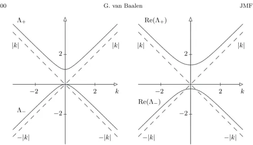
Linear stability analysis applied to the continuous Fourier transform y → k of (1.11) immediately shows that this dynamical system is ill posed, as two of the four eigenvalues of L(−ik, n) have positive real part growing to infinity as |k| → ∞ (see figure 1). In a linear setting (i.e. q = 0), we thus have to restrict the boundary conditions z(x0) to the linear center-stable manifold, that is to those
z(x0) satisfying z(x0) = Psz(x0) where Psis the projection on the stable modes
Λ+ Λ− Re(Λ+) Re(Λ−) −|k| −|k| −|k| −|k| |k| |k| |k| |k| k k 2 −2 −2 2 2 −2 2 −2
Fig. 1. (real part of the) eigenvalues of L(−ik, n) as a function of wavelength k, with nτ = 0 in left panel, and nτ = 1 in right panel.
parameterized by2 P
sz0 = LVw + LEν where w is a ‘vorticity-like’ function (of
y and t) and ν is a ‘velocity-like’ function (also of y and t). The mode LVw is
called ‘vorticity mode’ since the vorticity component3of L
Vw is w. The mode LEν
(associated with the eigenvalue −|k| of L(−ik)) is called ‘Eulerian’ mode, since LEν = (0, 0, ν, Hν) where H is the Hilbert transform on the boundary, and for
well behaved ν, we can construct a stream function Ψ, harmonic in Ω+, satisfying
∇Ψ|x=x0 = (ν, Hν). In the nonlinear setting, the boundary conditions have to
be restricted to the nonlinear center-stable manifold. In Section 2, we will show that this manifold can be implicitly defined using Duhamel’s variation of constants formula. Namely, we will cast (1.11) in an integral form given by
z(x) = eL(∂y)(x−x0)(L Vw + LEν) + Z x x0 d˜x eL(∂y)(x−˜x)P sq(˜x) − Z ∞ x d˜x eL(∂y)(x−˜x)(11 − P s)q(˜x). (1.12)
Evaluation of (1.12) at x = x0 then gives
z(x0) = LVw + LEν −
Z ∞ x0
d˜x eL(∂y)(x0−˜x)(11 − P
s)q(˜x), (1.13)
which accounts for the (small) nonlinear correction to the linear center-stable manifold.
2
Precise definitions of the operators LV and LEwill be given in Section 2. 3
A long wavelength expansion of LVw gives LVw ≈ (w, ∂y2w, −Iw, w) where I = ∂ −1 y , see
Before stating our main results in a precise manner (see Subsection 1.4 below), we need the definition of some functional spaces and related norms. On an informal level, our results are twofold. We will use the integral formulation (1.12) to prove that if w and ν are in a certain class Ci, there exist a (locally) unique solution of
(1.1) in the Banach space W defined in the next section. We will then show that the asymptotic structure of these solutions is indeed given by (1.8) with ϕ0 > 0.
On the other hand, time-periodic solutions of (1.2) must satisfy (1.1) for all x0
sufficiently large. We will then show that for solutions of (1.2) in a certain class Cu,
the q dependent terms in (1.12) are well defined, and thus solutions of (1.2) in Cu
must also satisfy (1.12) for certain functions w and ν. The functions w and ν can be determined by inverting any two of the four (linear and local) relations (1.13), the two remaining relations, which correspond to the central-stable manifold condition in the dynamical system formulation (1.11), being automatically satisfied since we know that the solution exist. We will then show that the functions w and ν obtained in this way are in the class Ci, which finally implies that solutions of (1.2) in Cu
also satisfy (1.3) with ϕ0> 0.
1.3. Definitions
We now define the topology we will use to control the decompositions (1.10). Let hxi = √1 + x2, ρ
β(y) = |y|β and f (x, y, t) = Pn∈Zeinτ tfn(x, y) for (x, y, t) ∈
[x0, ∞) × R × [0,2πτ ]. For p ≥ 1, we define |||f|||p,σ= sup x≥x0 kf(x)kp,σ, kf(x)kp,σ= hxiσkf(x)kp= hxiσ X n∈Z kfn(x, ·)kLp, |f(x)|p = sup n∈Zkfn(x, ·)kL p, kfkp,{σ 1,σ2}= sup x≥0hxi −σ1xσ2|f(x)| p,
where kfn(x, ·)kLp is the usual Lp-norm in the variable y and where we used the
notation kf(x)kp as a shorthand to the more rigorous kf(x, ·)kp. In the following,
we will use repeatedly the operators P0, P, Mn, I and S defined by
P0f = τ 2π Z 2π τ 0 dt f (t), ¡Pf¢(t) = f (t) − P0f, Mn(f ) = Z R ynf (y) dy (If)(y) = Z y −∞ dz f (z) 2 − Z ∞ y dz f (z)
2 , (Sf)(y) = f(y) + f(−y).
(1.14)
Note that I is the (formal) inverse of ∂y. We can now specify our basic functional
space.
Definition 1.1. Let C0∞ = ©{(un, vn, ωn)}n∈Z s.t. (un, vn, ωn) ∈ C0∞([x0, ∞) ×
R, R3) ∀n ∈ Zª. We denote by W the Banach space obtained by closure of C∞ 0
under the norm |||(u, v, ω)||| = |||u|||∞,1 2 + |||u|||q, 1 2− 1 q + |||∂yu|||r,1− 1 2r−η + |||v|||∞,1−ϕ+ |||v|||p,1−ϕ−1 p+ |||∂yv|||r,32−2r1−ξ + |||ω|||2,3 4 + |||ρβω|||2,34− β 2 + |||∂yω|||∞, 3 2 + |||∂yω|||1,1. (1.15)
We will also use the notation k(u(x), v(x), ω(x))k to denote the natural norm on the trace space at x obtained by replacing all ||| · |||p,σ by k · kp,σ in (1.15).
This choice is discussed at the end of this section. Note at this point that the ‘expected’ asymptotic decomposition (1.3) is in W if p > 1. We now specify the class of solutions of (1.2) for which our results can be applied:
Definition 1.2. A solution (u, v, ω) of (1.2) is in the class Cu(ρ) if |||(u, v, ω)||| ≤ ρ
for some finite constant ρ and
13 7 ≤ β ≤ 3, 1 < p ≤ q < 2, r > 2, 1 − 1 p < ϕ < r 1+2r, 0 ≤ η < 14− ϕ 2, min(ϕ, η) ≤ ξ ≤ 1 2, 1 2+ ξ − η − 2ϕ > 0 hτ i τ ≤ hx0i ϕ, 1 2+ η − ξ − ϕ rw > 0. (1.16)
Our results are optimal if p and q are (very) close to 1 while η, ξ and ϕ are close to zero. To get bounds depending only on x0and not on the Strouhal number τ , we
added the condition hτ iτ ≤ hx0iϕ, which is only restrictive in the limit of vanishing
Strouhal number. This is not expected to occur for time-periodic solutions of (1.2), if the Hopf bifurcation picture of [5, 14, 16, 17] is correct. We now define the class Ci, consisting essentially of those functions w and ν for which the part of r.h.s. of
(1.12) depending on w, ν is in W (see Lemma 3.1, 3.3 and 3.6):
Definition 1.3. We say that ν and w are in the class Ci(ρ) if k(ν, Hν, w)k ≤ ρ for
parameters satisfying (1.16) and M0(P0w) = 0.
Note that M0(P0w) is always well defined if k(0, 0, w)k < ∞ since kwk1,1 2 ≤
k(0, 0, w)k (see Lemma A.1). In the case of symmetric flows (i.e. u even in y and v odd in y), M0(P0w) = 0 is a trivial consequence of the fact that w is an odd
function of y (it is also expected from (1.3) or (1.8)).
We end this section by making some comments on Definition 1.1. First, for the v component, we will need ϕ > 0. Namely, as we will see, the optimal decay rate for v as x → ∞ can only be obtained if Hν ∈ L1. But (apart from symmetric
flows), Hν(y) ∼ 1/y as y → ∞ (see (1.3)), so in general Hν 6∈ L1. The second
comment is on the need of η and ξ. Basically, the problem is that ∂yu and ∂yv are
naturally composed of sum of functions on two length scales (y ∼√x and y ∼ x, see e.g. (1.9)). Dependence on r of the decay exponents as x → ∞ of Lr norms
of such functions either vary like 1/(2r) for functions on the shorter scale or like 1/r for functions on the longer one. Our choice of exponents are thus ‘wrong’
on the scale y ∼ x and is ‘corrected’ by introducing η and ξ. These additional parameters would not be needed if we choose r = ∞, but in that case we would lose the boundedness of the Dirichlet–Neumann operator v → Hv in W, which is needed to compare solutions of (1.1) and (1.2) (see Section 7).
1.4. Main results
We are now in position to state our results in a precise manner. The first one states that the topology of Definition 1.1 is well adapted to (1.1):
Theorem 1.4.If x0 is sufficiently large, and ν and w are in the class Ci(ρ) with
parameters satisfying (1.16), then there exist ρ′> ρ and a (locally) unique solution
to (1.1) in Cu(ρ′) with parameters satisfying (1.16).
Once existence of solutions is proved, we give an intermediate result concerning the asymptotic properties of the vorticity and the first component of the velocity field:
Corollary 1.5. Let a1= (−M0(IP0w) −RΩ+P0(v(x, y)ω(x, y)) dxdy, 0, 0, 0, 0, 0)
and ua1, ωa1 as in (1.6) and (1.9), then for all ε > 0, solutions to (1.1) in Cu
satisfy for all 1
2 ≤ β0≤ 1 − 2(1 + ε)ϕ the estimates |||ω − ωa1|||1,1−(1+ε)ϕ+ |||ω − ωa1|||∞,3 2−(1+ε)ϕ≤ C |||ρβ0(ω − ωa1)|||2,5 4−β02−(1+ε)ϕ+ |||u − u a1|||∞,1−(1+ε)ϕ≤ C, (1.17) for some constant C which depends on x0, |||(u, v, ω)||| and k(ν, Hν, w)k.
Note that since ϕ > 0, in (1.3), the terms containing a2to a6are of smaller order
than the remainder, which explains why these parameters are not yet specified at this point. We will then be able to get the complete asymptotic form in the Corollary 1.6. Assume that kρ1
2v(x0)k4+kρ 1 2−(1+ε)ϕSνk1+kρ 1 2−(1+ε)ϕSHνk1< ∞ for some (1+ε)ϕ < 1
8. Let a1denote the first component of a1in Corollary 1.5,
a2= M0(Sν)−
R
Ω+P0(v(x, y)ω(x, y)) dxdy and a3= M0(SHν), then there exists
a constant a4 such that for a = (a1, a2, a3, a4, a21, a1P0a3), ua, va and ωa as in
(1.6) and (1.9), solutions to (1.1) in Cu(ρ) satisfy for all x ≥ x0 and ε > 0, the
estimate (1.17) and
|||u − ua|||∞,9
8−(1+ε)ϕ+ |||v − va|||∞,32−(1+ε)ϕ ≤ C (1.18)
for some constant C which depends on x0, |||(u, v, ω)||| and k(ν, Hν, w)k.
As a first comment to this result, we want to note that we stopped at the stated asymptotic order in Corollary 1.6 for concision, but our method is constructive and
could be systematically used to get higher order asymptotics. We also believe that (1.17) and (1.18) should hold with ϕ = 0 if ua, vaand ωacontain appropriate
loga-rithmic corrections. More interesting is the question of the actual decay rate of the first non-trivial time-periodic component. In our setting, we cannot even exclude that this decay rate is x−1. Namely, as we motivated at the end of Section 1.1,
we have no rigorous evidence but only strong physical motivations to believe that in the ‘usual’ problem (1.2) in an exterior domain, a2 and a3are constant in time
(in our setting, this follows if M0(Sν) and M0(SHν) are so). Though linear
analysis (see also figure 1) indicates that the time harmonic of order n 6= 0 of the ‘vorticity mode’ associated with Λ− should decay exponentially in the wake, this quantity is slaved to an inhomogeneous nonlinear term built from the n = 0 harmonic of the vorticity and the nth harmonic of an ‘Eulerian mode’ (associated
with the eigenvalue −|k|), both modes decaying only algebraically as x → ∞. We thus conjecture that the first non-trivial time-periodic part will appear in the next (few) term(s) in the development.
It remains to show that the functional settings in which Corollary 1.6 is proved is reasonable in the sense that its conclusions are also true for the well known stationary solutions of the ‘usual’ exterior problem (1.2). To do so, we first note that
Proposition 1.7.For any stationary solution of (1.2) “Physically Reasonable” (PR) in the sense of Finn and Smith (see e.g. [6, 7, 8]), the fields u, v and ω satisfy |||(u, v, ω)||| ≤ C with parameters satisfying (1.16) if x0 is sufficiently large.
Furthermore kρ1
2v(x0)k4 and kρ 1
2−(1+ε)ϕSv(x0)k1 are bounded for all ε > 0.
and then conclude that
Theorem 1.8.Assume that there exist a unique solution to (1.1) in Cu(ρ′) with
parameters satisfying (1.16), then if x0 is sufficiently large, ν and w are in the
class Ci(ρ) with parameters satisfying (1.16). If additionally kρ1
2v(x0)k4 and
kρ1
2−(1+ε)ϕSv(x0)k1 are bounded, then for all ε > 0, it holds
kρ1
2−(1+ε)ϕSνk1+ kρ12−(1+ε)ϕSHνk1≤ C1(x0, |||(u, v, ω)|||). (1.19)
From this theorem, Proposition 1.7 and the (local) uniqueness of the solutions in Cu, we conclude that (PR) solutions satisfy the integral formulation (1.12) and
the hypotheses of Corollary 1.6, which proves that its conclusions also hold for (PR) stationary solutions in the whole exterior domain.
1.5. Structure of the paper
Our first task in the remainder of this paper is to explicit the integral formulation (1.12). This is done in the next section (Section 2). The integral formulation is
then used in Section 3 to prove Theorem 1.4, in Section 4 to prove Corollary 1.5 and in Section 5 to prove Corollary 1.6. The proof of Proposition 1.7 is delayed until Section 6, while that of Theorem 1.8 is delayed until Section 7.
2. Integral formulation
We now derive an explicit formula for the integral formulation (1.12) of the solution of (1.1) and (1.11). All the material of this section is very similar to [9, 18] where the case τ = 0 was treated. For completeness, we now reproduce some of the analysis here, encompassing the additional term proportional to the Strouhal number τ .
For further reference, we first note that the representation (1.11) with q = uη + v∂yω is not the only possibility. Namely, using the incompressibility relation
∂xu = −∂yv and the definition of the vorticity, we may cast the nonlinearity q in
the following equivalent and more useful forms
q = ∂x(uω) + ∂y(vω) ≡ ∂x(P ) + ∂y(Q) = (∂x2+ ∂2y)R + 2∂yQ,
since P = uω = ∂xR + ∂yS and Q = vω = −∂yR + ∂xS where R = uv, S = 1
2(v
2−u2). We then note that performing a (continuous) Fourier transform4f (k) =
R
Re
ikyf (y) leads for each n ∈ Z to a system of the form ∂
xzn= L(−ik, n)zn+ qn,
with z = (ω, η, u, v), q = (0, q, 0, 0). As in [9], the matrix L(−ik, n) can be diagonalized. Namely, define σ(k) = sign(k), Λ0 =
p
1 + 4(k2+ inτ ) and Λ ± = 1±Λ0
2 , and set z = S−1y, with y = (ω+, ω−, u+, u−) and
S(−ik, n) = 1 1 0 0 Λ+ Λ− 0 0 ik Λ++inτ ik Λ−+inτ 1 1 Λ+ Λ++inτ Λ−
Λ−+inτ −iσ iσ
,
then we get S(−ik, n)−1L(−ik, n)S(−ik, n) = diag(Λ
+, Λ−, |k|, −|k|) (see figure
1 for a graphical display of the dispersion relations). The symbols of the opera-tors LV, resp. LE used in Subsection 1.2 to characterize the linear center-stable
manifold are the second, resp. fourth column of S, since the two equations corre-sponding to the ‘+’ modes are linearly unstable (the real part of Λ+ is positive).
Integrating the unstable modes backwards from x = ∞, where we set them to 0 (see also [18]), we get
ω+(x) = − Z ∞ x d˜xe Λ+(x−˜x) Λ0 q(˜x) ω−(x) = eΛ−(x−x0)ω˜ 0− Z x x0 d˜x e Λ−(x−˜x) Λ0 q(˜x)
4 We distinguish functions and their Fourier transform only from their arguments ‘k’, resp. ‘y’
u+(x) = − 1 2 Z ∞ x d˜x e|k|(x−˜ x) ik − nτσq(˜x) u−(x, k) = e−|k|(x−x0)u˜ 0+ 1 2 Z x x0 d˜x e−|k|(x−˜ x) ik + nτ σ q(˜x),
for some functions ˜ω0 and ˜u0 to be specified. Integrating by parts the integrals
involving ∂xP in ω±, replacing q = (∂x2+ ∂2y)R + 2∂yQ in u± and integrating twice
by parts the term involving ∂x2R, we find
ω+(x) = P (x) Λ0 − Z ∞ x d˜x e Λ+(x−˜x) Λ0 q+(˜x) ω−(x) = eΛ−(x−x0)w −P (x) Λ0 − Z x x0 d˜x e Λ−(x−˜x) Λ0 q−(˜x) u+(x) = P (x) + ikS(x) + |k|R(x) 2(ik − nτσ) + Z ∞ x d˜x ike|k|(x−˜ x) ik − nτσ Q(˜x) u−(x) = e−|k|(x−x0)ν +P (x) + ikS(x) − |k|R(x) 2(ik + nτ σ) − Z x x0 d˜x ike−|k|(x−˜ x) ik + nτ σ Q(˜x), where q±= Λ±P − ikQ, ν(k) = ˜u0(k) −P (x0)+ikB(x2(ik+nτ σ)0)−|k|A(x0) and w(k) = ˜ω0(k) + P (x0)
Λ0 . Then, a little algebra shows that when reconstructing ω, u and v, the terms
involving P (x) cancel out exactly. We thus find, after inverse Fourier transform u(x) = uL(x) + uN(x), v(x) = vL(x) + vN(x)
ω(x) = ωL(x) + ωN(x),
(2.1) with uL(x) =P2i=1uL,i(x), vL(x) =Pi=13 vL,i(x), uN(x) =P6i=1uN,i(x), vN(x) =
P8
i=1vN,i(x) and ωN(x) =P4i=1ωN,i(x), where vN,7(x) = ωN,1(x) + ωN,2(x) +
ωN,3(x), vN,8(x) = ωN,4(x), and uL,1(x) = K1(x − x0)Luw, vL,1(x) = K1(x − x0)(Lv− 11)w, ωL(x) = K1(x − x0)w, uL,2(x) = K0(x − x0)ν, vL,2(x) = K0(x − x0)Hν, vL,3(x) = ωL(x), uN,1(x) = −J1[K8, Q](x), uN,2(x) = −J1[K12, Q](x), uN,3(x) = J1[K2− K9, P ](x), uN,4(x) = J2[K12∗ , Q](x), (2.2) vN,1(x) = J1[K9, Q](x), vN,2(x) = J1[K13, Q](x), vN,3(x) = J1[K10+ K11, P ](x), vN,4(x) = −J2[K13∗, Q](x), (2.3) uN,5(x) = J2[E(K2− K4), P ](x) − J2[EK3, Q](x), vN,5(x) = −J2[EK5, P ](x) + J2[EK4, Q](x), uN,6(x) = L1S(x) − L2R(x), vN,6(x) = −L1R(x) − L2S(x), ωN,1(x) = −J1[K2, Q](x), ωN,2(x) = −J1[K6, P ](x),
ωN,3(x) = −J1[K7, P ](x), ωN,4(x) = −J2[E(K1+ K6+ K7), P ](x) − J2[EK2, Q](x), where J1[K, f ](x) = Z x x0 d˜x K(x − ˜x) f(˜x), J2[K, f ](x) = Z ∞ x d˜x K(˜x − x) f(˜x) and, in terms of their symbols,
L1=
k2
k2+ (nτ )2, L2=
|k|nτ
k2+ (nτ )2, Lu= (Λ−+ inτ )−1ik, Lv= (Λ−+ inτ )−1Λ−,
and for i = 0, . . . , 13, Ki(x) is the convolution operator with the inverse Fourier
transform of Ki(x, k) and (EKi)(x) with that of e−xKi(x, k), where
K0(x, k) = e−|k|x K1(x, k) = eΛ−x K2(x, k) = −ikeΛΛ−x0 K3(x, k) = k 2eΛ−x Λ0(Λ++inτ ) K4(x, k) = knτ eΛ−x Λ0(Λ++inτ ) K5(x, k) = − inτ Λ+eΛ−x Λ0(Λ++inτ ) K6(x, k) =Re(ΛΛ0−)eΛ−x K7(x, k) = iIm(ΛΛ0−)eΛ−x K8(x, k) = k 2eΛ−x Λ0(Λ−+inτ )
K9(x, k) =Λ0knτ e(Λ−Λ−x+inτ ) K10(x, k) = inτ Re(Λ−)e
Λ−x Λ0(Λ−+inτ ) K11(x, k) = −nτ Im(Λ−)eΛ−x Λ0(Λ−+inτ ) K12(x, k) =ike −|k|x ik+nτ σ K13(x, k) = |k|e −|k|x ik+nτ σ .
Various estimates of these kernels are given in Appendix A. Intuitively, the two kernels K12 and K13 behave like Poisson’s kernels π1x2+yx 2 and
1 π
y
x2+y2, while
all the other kernels behave like y derivatives or primitives of K1according to the
expansion of their pre-factor as |k| → 0 or |k| → ∞. We thus need to understand the basic properties of K1. To do so, we define
b(α) = 1 4 ³ 1 − q 1+√1+16α2 2 ´ , c(α) = 1 2 q 1+√1+16α2 2+32α2 ,
and note that (see also figure 1 on page 300) Re(Λ−) ≤ ( b(nτ ) − c(nτ)k2 ∀|k| ≤ 1 b(nτ ) −|k|2 ∀|k| ≥ 1 and ¯ ¯ ¯ ¯ 1 Λ0 ¯ ¯ ¯ ¯ ≤ ( (1 + (nτ )2)−1/4 (1 + k2)−1/2 .
The kernel K1corresponding to eΛ−xthus behaves like a superposition of a kernel
of Poisson’s type with a heat kernel (see also Lemma A.10): K1(x, y) ≈ eb(nτ )x ³ e− y2 4c(nτ )x √ 4πc(nτ ) x+ 1 π 2x x2+4y2 ´ . (2.4)
Most results of Appendix A can be easily derived from this analogy, in particular we see in (2.4) that ∂m
y K1 ∼ x−mhxi
m
2K1 and that since b(0) = 0 and b(τ ) < 0,
Lp estimates on K1 will decay at most algebraically as x → ∞, while the same
estimates on PK1 will decay exponentially faster.
Unfortunately, without using (yet unknown) compensations between the vari-ous terms in (2.1), we cannot conclude from this last remark that e.g. Pω will decay
exponentially as x → ∞. Namely, we first note that e.g. P(ωN,2(x) + ωN,3(x)) ≈
PP (x) as the integral defining P(ωN,2+ ωN,3) is dominated by the contribution
of the region ˜x ≈ x. Then, we note that PP (x) = ¡P0ω(x)¢¡Pu(x)¢+ . . ., and
that both P0ω and Pu decay at most algebraically because P0K1 and PuL,2 do
so (unless Pν = 0, in which case a more refined analysis shows that e.g. PuN,2
necessarily decays algebraically).
3. ‘Evolution’ estimates and the proof of Theorem 1.4
Our next task is to prove Theorem 1.4, which states that for each boundary data in Ci, there exists in Cu a (locally) unique solution to (2.1). The proof follows
easily from the contraction mapping principle. For fixed ν and w in Ci, we define
the map F : W → W by F(v, ω) = r.h.s. of (2.1). In the remainder of this section, we will prove that if the parameters satisfy (1.16), then there exists κ > 0, such that for all ui, vi and ωi, i = 1, 2 with |||(ui, vi, ωi)||| ≤ ˜ρ, we have
|||F(ui, vi, ωi)||| ≤ C1k(ν, Hν, w)k + C2hx0i−κρ˜2,
|||F(u1, v1, ω1) − F(u2, v2, ω2)||| ≤ C2hx0i−κ|||(u1− u2, v1− v2, ω1− ω2)||| ˜ρ.
Let ρ > 0 and 0 < ε < 12. If k(ν, Hν, w)k ≤ ρ and hx0i >¡C1C2ρε−1¢
1 κ
, the map F is a contraction in B0((1+ε)C1ρ) ⊂ W. By classical arguments, the approximating
sequence (un+1, vn+1, ωn+1) = F(un, vn, ωn) for n > 1 and (u1, v1, ω1) = F(0, 0)
converges to the unique solution of (1.1) in B0((1 + ε)C1ρ) ⊂ W. The proof of
Theorem 1.4 is thus completed, provided we prove the above estimates on F. This part of the proof is split between the next subsections as follows: Subsection 3.2 is devoted to the terms uL,i, vL,i and ωL and Subsection 3.3 to the terms uN,i,
vN,iand ωN,i. In the remainder of this section, the letter C stands for a constant
which may change its value from instance to instance, but is independent of x0,
|||(u, v, ω)||| and k(ν, Hν, w)k. 3.1. Preliminaries
In this whole section, we will use that for K a convolution kernel (in the variable y) acting on a function f (of y) and p11 + q11 = p12 +q12 = 1 + 1s, we have (see Subsection 1.3 for the definitions of the norms)
kρβKf k2≤ |ρβK|2kfk1+ |K|1kρβf k2, (3.1) kKfks≤ min ³ |K|p1kfkq1, |K|p2kfkq2 ´ . (3.2)
We will also use variants of (3.1) and (3.2) following from Kf = ∂yKIf and
∂y(Kf ) = (∂yK)f = K(∂yf ). In particular, (3.1)–(3.2) and their variants give a
and difficulty will be to get optimal decay rates as x → ∞. As a rule (particularly in Subsection 3.3), we will choose p1 as small as possible to cover regions where
the x argument of K is small and p2 as large as possible in regions where that
argument is large. For concision, we will often omit the arguments in the K’s and f ’s when no confusion is possible. For the same reason, we will use (3.1)–(3.2) without reference or even sometimes without explicit statement of the choice made for the parameters.
We also note for further reference that using kfk∞ ≤ (kfk2k∂yf k2)
1 2, the
interpolation inequality, 0 < ϕ < 1 2 and
1
2+ η − ξ ≥ 0, we have for some constant
C that
|||(f, 0, 0)||| ≤ C|||(0, f, 0)||| ≤ C|||(0, 0, f)|||, (3.3) and that the nonlinearities R, S, P and Q satisfy
|||P |||m,3 2−2m1 + |||∂yP |||n,2−2n1 −η+ |||ρβP |||2,54− β 2 ≤ C|||(u, v, ω)||| 2, |||Q|||m,2−ϕ− 1 2m + |||ρβQ|||2,74−ϕ− β 2 + |||∂yQ|||n, 5 2− 1 2n−ξ≤ C|||(u, v, ω)||| 2, |||R|||m,3 2−ϕ−m1 + |||∂yR|||r,32−η−2r1+ ≤ C|||(u, v, ω)||| 2, |||S|||m,1−1 m + |||∂yS|||r,32−η−2r1 ≤ C|||(u, v, ω)||| 2, (3.4)
for all 1 ≤ m ≤ ∞ and 1 ≤ n ≤ r. To establish (3.4), we used |||ω|||∞,1+ |||ω|||1,1 2 ≤ |||(0, 0, ω)|||, since kωk1 ≤ Cβkωk1− 1 2β 2 kρβωk 1 2β
2 and kωk2∞ ≤ kωk2k∂yωk2, see also
Lemma A.1.
3.2. The ‘linear’ terms
In this subsection, we prove that |||(uL, vL, ωL)||| ≤ Ck(ν, Hν, w)k provided ν and
w are in the Class Ci of Definition 1.3. By (3.3), it will be sufficient to prove that
|||(uL,1+ uL,2, vL,1+ vL,2, ωL)||| ≤ Ck(ν, Hν, w)k. For convenience, this inequality is
split component-wise in three following Lemmas. The general idea of the proofs is to consider separately the regions x0≤ x ≤ 2x0and x ≥ 2x0. In the first region, we
will use the fact that |K0(x − x0)|1+ |K1(x − x0)|1is uniformly bounded (thus K0·
and K1· are Lp-bounded operators for all p ≥ 1), whereas in the region x ≥ 2x0,
we will essentially use that |K0(x − x0)|p+ |K1(x − x0)|pdecays as x → ∞ as soon
as p > 1.
Lemma 3.1.If (1.16) holds, then there exists a constant C such that |||(0, 0, ωL)|||
≤ Ck(0, 0, w)k.
Proof. We first note that since |K1|1≤ C, we have
|||ωL|||2,3 4 ≤ C sup x0≤x≤2x0 hxi34kwk 2+ sup x≥2x0 hxi34¡|∂ yK1|2kP0Iwk1+ |PK1|2kwk1 ¢
≤ C(kwk2,3
4 + kwk1, 1
2 + kP0Iwk1),
where we used Lemma A.5, that x − x0 ≥ x2 if x ≥ 2x0, and that hxi
1
2eb(τ )x ≤
hτ i
τ ≤ hx0i
1
2. Omitting the details for concision, we get by the same arguments
that |||∂yωL|||∞,3 2 + |||∂yωL|||1,1 ≤ C(k∂ywk∞, 3 2 + k∂ywk1,1+ kwk1, 1 2 + kP0Iwk1).
Next, we note that for all z ∈ R, we can write ρβ(y) = ρβ(y − z) + L(y, z) with
|L(y, z)| ≤ C(ρβ(z) + ρ1(z)ρβ−1(y − z)), so that (here we use that β > 32)
|||ρβPωL|||2,3 4− β 2 ≤ Ckρβwk2, 3 4− β 2 + C supx≥x 0 hxi34− β 2|P ρ βK1|2kwk1 ≤ Ckρβwk2,3 4− β 2 + Ckwk1, 1 2, |||ρβP0ωL|||2,3 4− β 2 ≤ C sup x≥x0 hxi34− β 2 ³ k(ρβK1)P0wk2+ kρβwk2+ |ρβ−1K1|2kρ1wk1 ´ ≤ C³ sup x≥x0 hxi34− β 2|∂y(ρβK1)|2kIP0wk1 ´ + Ck(0, 0, w)k,
where we used k(ρβK1)P0wk2= k(∂yρβK1)IP0wk2and that since β > 32, we have
kρ1wk1,3 4− β 2 ≤ kwk2,34− β 2 + kρβwk2,34− β 2 ≤ k(0, 0, w)k. (3.5)
The proof is completed using kwk1,1
2 ≤ k(0, 0, w)k and Lemma 3.2 below. ¤
Lemma 3.2.Let β > 3 2 and 0 ≤ γ < β − 3 2, Zβ = {k(1 + ρβ)f k2 < ∞ and M0(f ) = R
Rf (y)dy = 0}. Then there exist constants Cβ, Cβ,γ such that for all
f ∈ Zβ, kIfk∞≤ Cβkfk 1− 1 2β 2 kρβf k 1 2β 2 and kργIfk1≤ Cβ,γkfk 1− 3 2β− γ β 2 kρβf k 3 2β+ γ β 2 .
The first inequality is also valid if M0(f ) 6= 0.
Proof. Let β > 3
2 and a > 0. Since kIfk∞ ≤ kfk1, the first inequality follows
from Lemma A.1. Then, since M0(f ) = 0, we have If(y) =
Rsign(y)∞
y dz f (z), so
that the proof follows easily from
|If(y)|2≤³akfk2+ kρβf k2
´2Z ∞ |y|
dz (a + |z|β)2,
the fact that R0∞dy |y|γ³R∞ y dz (1+|z|β)2 ´1 2 < ∞ if γ < β −3
2 and minimizing the
bound as a function of a. ¤
Lemma 3.3.If (1.16) holds, then there exists a constant C such that |||(uL,1, vL,1, 0)||| ≤ Ck(0, 0, w)k.
Proof. We first note that |||uL,1|||q,1 2− 1 2q≤|||uL,1|||1+|||uL,1|||∞, 1 2 and |||vL,1|||p,1− 1 2p−ϕ≤ |||vL,1|||1,1
2−ϕ+ |||vL,1|||∞,1−ϕ. Let ˜Lv = Lv− 11. We then note that ˜Lv =
−inτ Λ−+inτ,
in particular, P ˜Lv = ˜Lv and Pecb(nτ )x ≤ ecb(τ )x for all c > 0. As in Lemma 3.1,
since x − x0 ≥ x2 for x ≥ 2x0, b(τ ) < 0, hxie
b(τ )x 8 ≤ hτ i τ ≤ hx0i 1 2 and ξ ≥ ϕ, we have that |||vL,1|||1,1 2−ϕ+ ≤ C(k ˜Lvwk1, 1 2−ϕ+ sup x≥2x0 hxi12−ϕ|PK1|1k ˜Lvwk1≤ Ck ˜Lvwk 1,1 2−ϕ, |||vL,1|||∞,1−ϕ≤ Ck ˜Lvwk∞,1−ϕ+ sup x≥2x0 hxi1−2s1−ϕ|PK1|sk ˜Lvwk1, ≤ C(k ˜Lvwk1,1 2−ϕ+ k ˜Lvwk∞,1−ϕ), |||∂yvL,1|||r,3 2− 1 2r−ξ≤ k∂y ˜ Lvwkr,3 2− 1 2r−ξ+ C sup x≥2x0 hxi32− 1 2r−ξ|P∂yK1|rk ˜Lvwk1, ≤ C³k∂yL˜vωkr,3 2− 1 2r−ξ+ k ˜Lvωk1, 1 2−ϕ ´ . Then, proceeding as above, we get
|||(uL,1, 0, 0)||| ≤ C ¡ kLuwk1+ kLuwk∞,1 2 + k∂yLuwkr,1− 1 2r−η ¢ .
The proof is then completed using Lemma 3.4 and 3.5 below. ¤ Lemma 3.4(Mikhlin–H¨ormander). Let m : R → C, and assume that the follow-ing quantities are bounded: m0= sup
k∈R|m(k)| + |k∂
km(k)| and m1= sup k∈R|∂
km(k)|.
Let F denote the (continuous) Fourier transform and M : f → F−1m(·)Ff. Then
there exist constants Cp such that for all 1 < p < ∞, it holds
kMfk∞≤ C∞m0 ¡ kfk2k∂yf k2 ¢1 2, kMfkp≤ Cpm0kfkp kMfk1≤ C1 ³ m0 ¡ kfk2kρ1f k2 ¢1 2 +¡m 0m1 ¢1 2 kfk2 ´ .
Proof. The Lp estimate for 1 < p < ∞ is a consequence of the classical Mikhlin–
H¨ormander condition (see, e.g. [11]), the L∞ and L1 estimates are immediate
consequences of Sobolev’s and Plancherel’s inequalities. ¤ Lemma 3.5.Let ˜Lv= Lv− 11 and ˜Lu= Lu+ IP0 and assume that (1.16) holds,
then kLuwk1+ kLuwk∞,1 2 + k∂yLuwkr,1− 1 2r−η≤ C(kIP0wk1+ k(0, 0, w)k), k ˜Luwk1+ k ˜Luwk∞,1 2 + k∂y ˜ Luwkr,1−1 2r−η≤ Ck(0, 0, w)k, k ˜Lvwk1,1 2−ϕ+ k ˜Lvwk∞,1−ϕ+ k∂y ˜ Lvwkr,3 2−2r1−ξ≤ Ck(0, 0, w)k, kLvwk1,1 2−ϕ+ kLvwk∞,1−ϕ+ k∂yLvwkr, 3 2− 1 2r−ξ≤ Ck(0, 0, w)k.
Proof. The symbol T (k, n) of ˜Lu is given by T (k, n) = Λ−−ik+inτ if n 6= 0 and
T (k, 0) = −ik
Λ+, and it satisfies (uniformly in n ∈ Z) the hypothesis of Lemma 3.4
with m0= Chτ iτ ≤ Chx0i
1
2 and m1= Chτ i 2
τ2 ≤ Chx0i. Similarly, P ˜Lv satisfies the
hypothesis of Lemma 3.4 with m0 = 2hτ iτ ≤ 2hx0iϕ < 2hx0i
1
2 and m1 = m2
0 ≤
4hx0i2ϕ. The proof is then a straightforward application of ∂yIf = f, Lemma 3.2
and 3.4, inequality (3.5) and the fact that kwk1,1
2 + kwk∞,1≤ Ck(0, 0, w)kx0. ¤
Lemma 3.6.If (1.16) holds, then |||(uL,2, vL,2, 0)||| ≤ Ck(ν, Hν, 0)k and for all
x ≥ 2x0, we have kuL,2(x)k∞,1−ϕ+ kvL,2(x)k∞,1−ϕ≤ Ck(ν, Hν, 0)k.
Proof. We first note that |K0(x)|s ≤ Cx
1 s−1 and |∂yK0(x)|s≤ Cx 1 s−2. Then let q ≤ p0≤ ∞ and p ≤ p1≤ ∞, since (x − x0) 1 s−1 ≤ Chxi 1 s−1 if x ≥ 2x0, we get |||uL,2|||p0,12−p01 ≤ kνkp0,12−p01 + C sup x≥2x0 hxi12− 1 qkνk q, |||vL,2|||p1,1−p11−ϕ≤ kHνkp1,1−p11−ϕ+ C sup x≥2x0 hxi1−p1−ϕkHνk p, |||∂yuL,2|||r,1−1 2r−η≤ k∂yνkr,1−2r1−η+ C sup x≥2x0 hxi12− 1 qkνk q, |||∂yvL,2|||r,3 2− 1 2r−ξ≤ k∂yHνkr, 3 2− 1 2r−ξ+ C sup x≥2x0 hxi1−p1−ϕkHνk p,
while for x ≥ 2x0, we have
kuL,2(x)k∞+ kvL,2(x)k∞≤ hxi−1+ϕ sup x≥2x0
³
hxi1−p1−ϕ¡kνk
p+ kHνkp¢´
The proof is completed using Lemma 3.4, ξ ≥ ϕ, 1 ≤ q < 2 and 1 −1 p ≤ ϕ <
1 2. ¤
3.3. The nonlinear terms
In this section, we prove that there exist constants C and κ > 0 such that |||(uN, vN, ωN)||| ≤ Chx0i−κ|||(u, v, ω)|||2, (3.6)
This is the hardest part of the paper in that the parameters in (3.1)–(3.2) need to be chosen in the right way to get a bound that decays as x0→ ∞. The estimates of
the ‘local’ terms uN,6 and vN,6 are given in Proposition 3.8 below. The estimates
for the J1terms are split component-wise in Propositions 3.9, 3.10 and 3.11, those
for the J2 terms in Propositions 3.12, 3.13 and 3.14. During the course of these
proofs, we will encounter repeatedly the following functions Ahp2,q2,s p1,q1 i (x, x0) = Z x x0 d˜x min³ h˜xi−q 1 (x − ˜x)p1, hxish˜xi−q2 (x − ˜x)p2 ´ ,
Bhp2,q2,s2 p1,q1,s1 i (x, x0) = Z x x0 d˜x eb(τ )(x−˜4 x)min³ h˜xi −q1hx − ˜xis1 (x − ˜x)p1 , h˜xi−q2hx − ˜xis2 (x − ˜x)p2 ´ , which occur naturally from (3.1)–(3.2). These functions satisfy the
Lemma 3.7.Let p1< 1, s ≥ 0 and p2, q1, q2∈ R, there exists a constant C such
that for all x ≥ x0≥ 1, it holds
Ahp2,q2,s
p1,q1
i
(x, x0) ≤ C¡hxi1−q1−p1+ hxis−p2max(hxi1−q2, hx0i1−q2)¢, (3.7)
if q26= 1, while the same inequality holds with max(hxi1−q2, hx0i1−q2) replaced by
ln(1 + x) if q2 = 1. If furthermore we have s1, s2 ≥ 0 and hτ iτ ≤ hx0iϕ, then for
all m ≥ 0, there exists a constant C such that for all x ≥ x0≥ 1, it holds
Bhp2,q2,s2 p1,q1,s1 i (x, x0) ≤ C ³ hxi−q1hx 0i2(1+s1−p1)ϕ + hxi−p2−mhx 0i2(1+m+s2)ϕmax(hxi−q2, hx0i−q2) ´ . Proof. We first note that for all p > −1, there exists a constant C such that
Z x x0 d˜x eb(τ )(x−˜4 x)(x − ˜x)p≤ C Z ∞ 0 dz e−|b(τ )|z4 zp≤ Chx 0i2(1+p)ϕ, (3.8)
since |b(τ)| ≤ Cτ−2 ≤ Chx0i2ϕ. We then note that since x ≥ x
0 ≥ 1, we have hxi√
2 ≤ x ≤ hxi. We first consider the case of finite x, that is precisely, x0≤ x ≤ 2x0,
then Ahp2,q2,s p1,q1 i (x, x0) ≤ Chx0i−q1(x − x0)1−p1≤ Chx0i1−p1−q1, Bhp2,q2,s2 p1,q1,s1 i (x, x0) ≤ hx0i−q1 Z x x0 d˜x eb(τ )(x−˜4 x)(x − ˜x)s1−p1 ≤ Chx0i−q1+2(1+s1−p1)ϕ.
However, in the applications of this Lemma, we will generically have e.g. 1 − q1−
p1 < 0, that is, the integrals we seek to bound decay as x → ∞. To get the
optimal decay rate, the idea is to consider x ≥ 2x0, and split the integration
domain x0≤ ˜x ≤ x in two equal parts. Since x ≥ 2x0 implies x2 ≤ (x − x0) ≤ x
and x0≤ ˜x ≤ x+x2 0 implies x4 ≤x−x20 ≤ x − ˜x ≤ x − x0≤ x, we have
Ahp2,q2,s p1,q1 i (x, x0) ≤ Chxis−p2 Z x+x02 x0 d˜x h˜xi−q2+ Chxi−q1 Z x x+x0 2 d˜x (x − ˜x)−p1.
The proof of (3.7) is completed using Rx+x02
x0 d˜x h˜xi
−q2 ≤Rx
x0d˜x h˜xi
−q2 and
con-sidering separately q2< 1, q2= 1 and q2> 1. In the same way, we have
Bhp2,q2,s2 p1,q1,s1 i (x, x0) ≤C max(hxi −q2, hx 0i−q2) hxip2+m Z x+x0 2 x0 d˜x eb(τ )(x−˜4 x)(x − ˜x)s2+m
+ C hxiq1 Z x x+x0 2 d˜x eb(τ )(x−˜4 x)(x − ˜x)s1−p1,
which completes the proof with the help of (3.8). ¤
From now on, we begin the estimates on uN,i, vN,iand ωN,i. We first have the
Proposition 3.8.Assume that (1.16) holds, then for κ0= min(ϕ2,12− η + ξ − ϕ),
we have |||(uN,6, vN,6, 0)||| ≤ Chx0i−κ0|||(u, v, ω)|||2 and |||uN,6|||∞,1+ |||vN,6|||∞,1 ≤
C|||(u, v, ω)|||2.
Proof. The proof follows at once from Lemma A.3 and (3.4). ¤ Note that uN,6 and vN,6 decay faster than u and v as x → ∞. We then turn
to the estimates of ωN,1+ ωN,2+ ωN,3. To prepare the ground for the asymptotic
results of Section 4, we also show that ωN,2 and ωN,3 decay faster than ω as
x → ∞.
Proposition 3.9.If (1.16) holds, then there exists a constant C such that for κ1,1 = min(14−ϕ2 − η,12− ξ), we have |||(0, 0, ωN,1+ ωN,2+ ωN,3)||| ≤ Chx0i−κ1,1|||(u, v, ω)|||2, |||ωN,2|||∞,3 2−ϕ+ |||ωN,2|||1,1−ϕ+ |||ρβωN,2|||2,54− β 2−ϕ≤ C|||(u, v, ω)||| 2, |||ωN,3|||∞,3 2−ϕ+ |||ωN,3|||1,1−ϕ+ |||ρβωN,3|||2,54− β 2−ϕ≤ C|||(u, v, ω)||| 2.
Proof. We give the proof only for the case |||(u, v, ω)||| = 1, from which the general case follows immediately. From Appendix A and (3.1)–(3.2), it follows easily that
k(0, 0, ωN,1(x))k ≤ C ³ hxi34A h3 4, 3 2−ϕ,0 3 4, 3 2−ϕ i (x, x0) + hxi 3 4− β 2A h3 4− β 2, 3 2−ϕ,0 3 4− β 2, 3 2−ϕ i (x, x0) ´ + C³hxi34− β 2A h1 2, 7 4− β 2−ϕ,0 1 2,74− β 2−ϕ i (x, x0) ´ + C³hxi32A h2,3 2−ϕ,12 3 4, 9 4−ξ i (x, x0) + hxiA h3 2,32−ϕ,12 1 2,2−ξ i (x, x0) ´ . Using Lemma 3.7 and β ≥ 3
2, we get |||(0, 0, ωN,1)||| ≤ C ³ hx0i− 1 2+ϕ+ hx0i− 1 2+ξ ´ . Similarly, from Lemma A.6, it follows easily, choosing ξ2= 1 − ε1and ξ3= 2 − 2ε2
with εi> 0, that k(0, 0, ωN,2(x))k ≤ C ³ hxi34A h 1−ε1,54,0 1−ε1,54 i (x, x0) + hxi 3 4− β 2A h5 4− β 2,1,0 5 4− β 2,1 i (x, x0) ´ + C³hxi34− β 2A h 1−ε1,54− β 2,0 1−ε1,54− β 2 i (x, x0) ´ + C³hxi32A h2,3 2,12 1−ε2,74−η i (x, x0) + hxiA h2,1,1 2 1−ε1,32−η i (x, x0) ´ ,
kωN,2(x)k∞≤ CA h2,1,1 2 1−ε1,32 i (x, x0) ≤ C¡hxi− 3 2+ε1+ hxi−32ln(x)¢, kωN,2(x)k1≤ CA h1,1,0 1−ε1,1 i (x, x0) ≤ C ¡ hxi−1+ε1+ hxi−1ln(x)¢, kρβωN,2(x)k2≤ C ³ Ah54− β 2,1,0 5 4− β 2,1 i (x, x0) + A h1−ε 1,54− β 2,0 1−ε1,54− β 2 i (x, x0) ´ .
Let ˜κ(ε1, ε2) = min(12−ϕ,21−ε1−η,14−ε2−η). By Lemma 3.7, ln(1+x) ≤ Chxiϕ
and εi> 0, we get |||(0, 0, ωN,2)||| ≤ Chx0i−˜κ(ε1,ε2), (3.9) |||ωN,2|||∞,3 2−ε1+ |||ωN,2|||1,1−ε1+ |||ρβωN,2|||2,5 4− β 2−ε1 ≤ C. (3.10)
Finally, from Lemma A.7, it follows that k(0, 0, ωN,3(x))k ≤ C ³ hxi34B h3 4,1,0 3 4,1,0 i (x, x0) + hxi 3 4− β 2B h9 8− 3β 8,1, 3 8+ β 8 9 8− 3β 8,1,38+ β 8 i (x, x0) ´ + C³hxi34− β 2B h5 8,54− β 2,18 5 8, 5 4− β 2, 1 8 i (x, x0) ´ + C³hxi32B h2,1,1 2 3 4, 7 4−η,0 i (x, x0) + hxiB h13 8,1, 5 8 5 8, 3 2−η, 1 8 i (x, x0) ´ , kωN,3(x)k∞≤ CB h1,1,0 5 8,32,18 i (x, x0) ≤ Chxi− 3 2+ϕ, kωN,3(x)k1≤ CB h5 8,1,18 5 8,1,18 i (x, x0) ≤ Chxi−1+ϕ, kρβωN,3(x)k2≤ C ³ Bh98− 3β 8,1, 3 8+ β 8 9 8− 3β 8,1, 3 8+ β 8 i (x, x0) + B h5 8, 5 4− β 2, 1 8 5 8, 5 4− β 2, 1 8 i (x, x0) ´ , ≤ Chxi−54+ β 2+ϕ, (3.11)
where in (3.11), we used β ≥ 12. Using Lemma 3.7 and β ≥ 1, we get |||(0, 0, ωN,3)||| ≤
Chx0i−
1 4+
ϕ
2+η. Choosing ε1= ϕ and ε2=ϕ
2 in (3.9)–(3.10) completes the proof.
¤ We now turn to vN,1+ vN,2+ vN,3+ vN,7. For further reference, we also show
that some of these terms have improved decay rates compared to those of v. Proposition 3.10. If (1.16) holds, then there exists a constant C such that for κ1,2 = min(κ1,1,ϕ2,12− η + ξ − 2ϕ), we have
|||(0, vN,1+ vN,2+ vN,3+ vN,7, 0)||| ≤ Chx0i−κ1,2|||(u, v, ω)|||2, (3.12)
|||vN,1+ vN,3|||∞,3
2−ϕ ≤ Chx0i
ϕ|||(u, v, ω)|||2.
Proof. We give the proof only for the case |||(u, v, ω)||| = 1. Since vN,7(x) =
to (3.12) is already proved in Proposition 3.9. Then, from Lemmas A.8 and A.9, it follows easily that
|K10(x) + K11(x)|1≤ Ce b(τ )(x−˜x) 4 µ 1 x12 + hxi18 x18 + hxi18hx0iϕ x14 ¶ ≡ CB1(x), |K9(x)|1≤ Ce b(τ )(x−˜x) 4 ³ 1 +hx0iϕ x14 ´ ≡ CD1(x).
Let δs(x) = hxi−s, Bs(x) = J1[B1, δs](x) and Ds(x) = J1[D1, δs](x). We have
kvN,3(x)k∞≤ CB3 2(x), kvN,1(x)k∞≤ CD2−ϕ(x) and k(0, vN,3(x), 0)k ≤ Chxi1−ϕB3 2(x) + Chxi 1−ϕ−1 pB3 2− 1 2p(x) + Chxi32− 1 2r−ξB 2−1 2r−η(x), k(0, vN,1(x), 0)k ≤ Chxi1−ϕD2−ϕ(x) + Chxi1−ϕ− 1 pD 2−ϕ−1 2p(x) + Chxi32−2r1−ξD5 2− 1 2r−ξ(x).
Let ˜κ1,2 = min(12− ϕ,12− η + ξ − 2ϕ). Using Lemma 3.7, we get |||vN,3|||∞,3 2−ϕ+
|||vN,1|||∞,3
2−ϕ ≤ Chx0i
ϕ and |||(0, v
N,3, 0)||| + |||(0, vN,1, 0)||| ≤ Chx0i−˜κ1,2. In the
same way, from Lemma A.4, it follows easily that for all q > 1 and s ≥ 1, we have |∂yK13(x)|2≤ Cx− 3 2, |K 13(x)|q ≤ Cx−1+ 1 q ³ 1 +hx0i 1 4q x4q1 ´ ≡ CEq(x).
Then, let Eq,s(x) = J1[Eq, ρs](x). We have kvN,2(x)k∞,1−ϕ≤ Chxi1−ϕE1 ϕ,32− ϕ 2(x), kvN,2(x)kp,1−ϕ−1 p ≤ Chxi 1−ϕ−1 pE p,3 2−ϕ(x). Using χ = 3 2− 1 2r − ξ k∂yvN,2(x)kr,3 2−2r1−ξ≤ Chxi 3 2− 1 2r−ξ Z x x0 d˜x min³ E2(x − ˜x) h˜xi94− 1 2r−ξ , x˜ −7 4+2r1 (x − ˜x)32 ´ . Using Lemma 3.7 and r > 2, we get k(0, vN,2(x), 0)k ≤ Chx0i−
ϕ
2. ¤
We conclude this section by estimating uN,1 + uN,2+ uN,3. In the spirit of
Proposition 3.9, we will also show that some of these terms have improved decay rates as x → ∞.
Proposition 3.11. Assume that the parameters satisfy (1.16), then there exists a constant C such that for κ1,3 = min(κ1,2,12− (1 + 2r1)ϕ,12 − ξ + η −ϕr) and all
ε > 0, we have |||(uN,1+ uN,2+ uN,3, 0, 0)||| ≤ hx0i−κ1,3|||(u, v, ω)|||2, (3.13) |||uN,2+ uN,3|||∞,1−ϕ+ |||P(uN,1+ uN,3)|||∞,3 2 ≤ Chx0i 5ϕ 2 |||(u, v, ω)|||2.
Proof. We also give the proof only for the case |||(u, v, ω)||| = 1. We first note that |||(uN,2, 0, 0)||| ≤ |||(0, uN,2, 0)||| (see (3.3)), and that uN,2 and vN,2 differ only by
signs and the exchange of the Kernels K12 and K13. The bound on vN,2 in the
proof of Proposition 3.10 being insensitive to these details then applies mutatis mutandis, in particular, we have |||uN,2|||∞,1−ϕ ≤ C. Then, by Lemma A.8, we
have |K8(x)|p≤ Chxi 1 2− 1 2p x1−1p ³ 1 + hx0i ϕ p x4p1 ´ ≡ CEp(x), |K2(x)|p+ |K9(x)|p≤ C Ã 1 x1−2p1 +e b(τ )x 4 hxi 1 2− 1 2p x1−1p ³ 1 +hx0i ϕ p x4p1 ´! ≡ CHp(x), |∂yK2(x)|2+ |∂yK9(x)|2≤ C Ã hxi12 x74 +e b(τ )x 4 hxi 3 4 x32 ! ≡ CJ(x), so that kuN,1(x)kp0,12−p01 ≤ Chxi 1 2−p01 Z x x0 d˜x min³ E1(x − ˜x) h˜xi2−ϕ−2p01 ,Ep0(x − ˜x) h˜xi32−ϕ ´ k∂yuN,1(x)kr,1−1 2r−η≤ Chxi 1−1 2r−η Z x x0 d˜x min³ Er(x − ˜x) h˜xi2−ξ , hxi1−1 2rh˜xi− 3 2+ϕ (x − ˜x)2−1 r ´ , kuN,3(x)kp0 ≤ C Z x x0 d˜x min³h˜xi−32+2p01 H 1(x − ˜x), h˜xi−1Hp0(x − ˜x) ´ k∂yuN,3(x)kr,1−1 2r−η≤ Chxi 1−1 2r−η Z x x0 d˜x min³ Hr(x − ˜x) h˜xi32−η ,J(x − ˜x) h˜xi54−2r1 ´ . By Lemma 3.7, using these bounds with p0= q and p0= ∞, we get
|||(uN,1, 0, 0)||| ≤ C ³ hx0i− 1 2+ϕ+ hx 0i− 1 2+ξ−η+ ϕ r−4r1 ´ , |||(uN,3, 0, 0)||| ≤ C ³ hx0i− 1 2+ϕ+ hx 0i− 1 2− 1 2r+(1+ 3 2r)ϕ ´ , and |||uN,3|||∞,1−ϕ≤ C. We finally note that
kP(uN,1(x) + uN,3(x))k∞≤ C Z x x0 d˜x eb(τ )(x−˜4 x ³ 1 + 1 x12 + hx0i ϕ (x − ˜x)14 ´ h˜xi−32,
which shows that |||P(uN,1(x) + uN,3(x))|||∞,3
2 ≤ Chx0i 5ϕ
2 and completes the proof.
¤ We now turn to the estimates of J2 terms. For further reference, we will also
point out that most decay rates are in fact better than those of the related fields. We begin with the vorticity component:
Proposition 3.12. If (1.16) holds, then there exists a constant C such that for κ2,1 =14− η, we have |||(0, 0, ωN,4)||| ≤ Chx0i−κ2,1|||(u, v, ω)|||2 and
|||ωN,4|||∞,3
2 + |||ωN,4|||1,1+ |||ρβωN,4|||2,54− β
2 ≤ C|||(u, v, ω)|||
Proof. We give the proof only for the case |||(u, v, ω)||| = 1. From the results of Appendix A, it follows easily that there are exponents p ≥ 0 and q < 1 such that kK1+ K6+ K7k1,{p,q}, kK2k1,{p,q}, kK1+ K6+ K7k2,{p,q}, kK2k2,{p,q}, kρβ(K1+
K6+ K7)k1,{p,q} and kρβK2k1,{p,q} are all bounded by a constant. We then note
that, e.g. |||J2[EK2, Q]|||2,3 4 ≤ C sup x≥x0 Z ∞ x d˜x ex−˜ xh˜x − xip (˜x − x)q hxi 3 4kQ(˜x)k 2≤ Chx0iϕ−1,
which follows from sup ˜ x≥xhxi 3 4kQ(˜x)k2≤ |||Q||| 2,7 4−ϕsup ˜ x≥xhxi 3 4h˜xi− 7 4+ϕ≤ hxiϕ−1. (3.14)
Using similar estimates, β > 32, ϕ ≤ ξ < 12 and 1 2− ξ + η ≥ 0, we easily get |||(0, 0, ωN,4)||| ≤ Chx0iη− 1 4, |||ωN,4|||∞,3 2+ |||ωN,4|||1,1+ |||ρβωN,4|||2,54− β 2 ≤ C. ¤
Proposition 3.13. Let κ2,2 = min(κ2,1,ϕ2). If (1.16) holds, then there exists a
constant C such that for all 0 < ε ≤ 1, we have
|||(0, vN,4+ vN,5+ vN,8, 0)||| ≤ Chx0i−κ2,2|||(u, v, ω)|||2,
|||vN,4+ vN,5+ vN,8|||∞,3
2−(1+ε)ϕ≤ C|||(u, v, ω)|||
2. (3.15)
Proof. We give the proof only for the case |||(u, v, ω)||| = 1. Since vN,8(x) = ωN,4(x),
we see again that using (3.3), the contribution of ωN,4 to (3.15) is already proved
in Proposition 3.12. We then proceed as in Proposition 3.12. There are exponents p ≥ 0, q < 1 and s > 1 such that kK4k1,{p,q}+ kK5k1,{p,q}≤ C and for x ≤ ˜x,
kP0K13ks,{0,1−1 s}≤ C, kPK13ks,{0,1−4s3}≤ Chx0i 1 4s ≤ Ch˜xi4s1, where we used τ−1 4s ≤ hτi− 1 4shx0i ϕ 4s ≤ hx0i 1
4s in the last inequality. Then, for all
x ≥ x0, we have (as in (3.14) above)
sup ˜ x≥x ³ hxi1−ϕkP (˜x)k∞+ hxi1−ϕ− 1 pkP (˜x)k p+ hxi 3 2−2r1−ξk∂ yP (˜x)kr ´ ≤ Chxi−12, sup ˜ x≥x ³ hxi1−ϕkQ(˜x)k ∞+ hxi1−ϕ− 1 pkQ(˜x)k p+ hxi 3 2−2r1−ξk∂ yQ(˜x)kr ´ ≤ Chxi−1 2, since ϕ ≤ ξ <1
2 and η ≤ ξ. As in Proposition 3.12, we thus get |||vN,5|||∞,3 2−ϕ ≤ C
and for all 0 < ε ≤ 1,
|||(0, vN,5, 0)||| ≤ Chx0i− 1 2 sup x≥x0 Z ∞ x d˜x ex−˜ xh˜x − xip (˜x − x)q , kvN,4(x)k∞,1−ϕ≤ Chxi− 1 2+εϕ Z ∞ 1 dz z− 3 2+(1−ε)ϕ (z − 1)1−2εϕ ¡ 1 + (z − 1)−ϕ4¢,
kvN,4(x)kp,1−ϕ−1 p ≤ Chxi −1 2 Z ∞ 1 dz z− 3 2+ϕ (z − 1)1−p1 ¡ 1 + (z − 1)−4p1¢, k∂yvN,4(x)kr,3 2− 1 2r−ξ≤ Chxi −1 4 Z ∞ 1 dz z−94+ 1 2r+η¡(z − 1)− 1 2 + (z − 1)− 5 8¢,
where we used the change of variables ˜x = xz in the three last inequalities. ¤ Proposition 3.14. Let κ2,3 = κ2,2. If (1.16) holds, then there exists a constant C
such that for all 0 < ε ≤ 1, it holds |||(uN,4+ uN,5, 0, 0)||| ≤ Chx0i−κ2,3|||(u, v, ω)|||2
and
|||uN,4+ uN,5|||∞,3
2−(1+ε)ϕ ≤ C|||(u, v, ω)|||
2.
Proof. We give the proof only for the case |||(u, v, ω)||| = 1. We first note that kK2k1,{0,1
2}+ kK3k1,{0,12}+ kK4k1,{0,12}≤ C, while for all x0≤ x ≤ ˜x, using (3.4),
we have sup ˜ x≥x ³ hxi12kP (˜x)k ∞+ hxi 1 2−1pkP (˜x)k p+ hxi1− 1 2r−ηk∂yP (˜x)kr ´ ≤ Chxi−1 sup ˜ x≥x ³ hxi12kQ(˜x)k ∞+ hxi 1 2−1pkQ(˜x)k p+ hxi1− 1 2r−ηk∂yQ(˜x)kr ´ ≤ Chxi−1, since ϕ ≤ ξ < 1 2 and 1
2− ξ + η ≥ 0. Proceeding as in the proof Proposition 3.13,
we easily get |||(uN,5, 0, 0)||| ≤ Chx0i−κ2,3 and |||uN,5|||∞,3
2−(1+ε)ϕ ≤ C. Next, we
use (3.3) and note that uN,4and vN,4 differ only by signs and the exchange of the
Kernels K12 and K13 (see (2.3) and (2.2)). The bounds on vN,4 in the proof of
Proposition 3.13 being insensitive to these details then apply mutatis mutandis. ¤
4. Asymptotics
We now turn to the asymptotic description of the (locally) unique solutions of (1.1) in Cu. As explained in Subsection 1.5, we will first prove the partial description
of Corollary 1.5, before turning to the full description in Section 5. To avoid the unnecessary proliferation of symbols, in this section, the letter C stands for a constant which may change its value from instance to instance and depends on x0, k(ν, Hν, w)k and |||(u, v, ω)|||. We will prove (1.17) only for x ≥ 2x0, as the
estimates are trivially satisfied otherwise.
The proof of Corollary 1.5 is given in the next subsection. Its basis is that the large time asymptotics of K1(x)f is captured by5 M0(f )K1(x) if f decays
sufficiently fast, which is the content of the next Lemma.
5
Lemma 4.1.Let 0 ≤ γ ≤ 1, 0 ≤ γ2≤ 2. Let ¡ R1f ¢ (x) = K1(x)(f − M0(f )) − ∂yK1(x)M1(f ), ¡ R2f¢(x) = K1(x)(f − M0(f )) ¡ R3f¢(x) = K8(x)(f − M0(f )) − ∂yK8(x)M1(f ).
Then for all m ≥ 0 and 2 ≤ s ≤ ∞, there exist constants Cγ, Cγ2 such that
k∂m y ¡ R2f¢(x)ks≤ Cγhxi 1 2−2s1+ m+γ 2 x1−1 s+m+γ kρ γf k1, k∂ym ¡ R2f ¢ (x)k1≤ Cγhxi 3+γ 4 + m 2 x1+m+γ2 (kρ1f k1kργf k1) 1 2, kρ1∂ym ¡ R2f ¢ (x)k2≤ Cγhxi 5 4+ m 2 x32+m kρ 1f k1, k¡R1f¢(x)k∞+ k¡R3f¢(x)k∞≤ Cγ2 hxi1+γ22 x1+γ2 kργ2f k1.
Proof. Using twice the Fourier Transform, we get (with i = 1 or i = 3) e.g. k¡Rif ¢ (x)k∞≤ X n∈Z Z ∞ −∞ dk ¯¯|k|γ2eΛ−x¯¯ Z ∞ −∞ dy ¯ ¯ ¯ ¯ eiky− 1 − iky |ky|γ2 ¯ ¯ ¯ ¯ |y| γ2|f n(y)|, k∂ym ¡ R2f ¢ (x)k∞≤ X n∈Z Z ∞ −∞ dk ¯¯|k|m+γeΛ−x¯¯ Z ∞ −∞ dy ¯ ¯ ¯ ¯ eiky− 1 |ky|γ ¯ ¯ ¯ ¯ |y| γ |fn(y)|,
and similar estimates for k∂m y
¡
R2f¢(x)k2 and kρ1∂ym
¡
R2f¢(x)k2. The proof is
completed using Lemma A.2 and k∂m
y R2f k1≤ ¡ k∂m y R2f k2kρ1∂ymR2f k2 ¢1 2. ¤
4.1. The proof of Corollary 1.5
Let a1,1 = −M0(IP0w), a1,2 = RΩ+P0Q(x, y) dxdy, a1,1 = (a1,1, 0, 0, 0, 0, 0),
a1,2= (−a1,2, 0, 0, 0, 0, 0) and a1= a1,1+a1,2. Define uL,4(x) = −K1(x−x0)IP0w
and ωL,1(x) = ∂yK1(x − x0)IP0w. We have
u(x) − ua1(x) = 6 X i=1 Ui(x), ω(x) − ωa1(x) = 6 X i=1 Wi(x) where U1(x) = uL(x) − uL,4(x), U2(x) = uL,4(x) − ua1,1(x − x0) U3(x) = ua1,1(x − x0) − ua1,1(x), U4(x) = uN(x) − P0uN,1(x), U5(x) = P0uN,1(x) − ua1,2(x − x0), U6(x) = ua1,2(x − x0) − ua1,2(x)
and a mirror definition of Wi, i = 1, . . . , 6. We complete the proof of Corollary 1.5
by proving that for all ε > 0, there exists a constant C such that kUi(x)k∞,1−(1+ε)ϕ+ kWi(x)k∞,3
2−(1+ε)ϕ≤ C,
kWi(x)k1,1−(1+ε)ϕ+ kρβ0Wi(x)k2,5
4−β02−(1+ε)ϕ≤ C
(4.1) for all i = 1, . . . , 6, x ≥ 2x0 and 12 ≤ β0 ≤ 1 − 2(1 + ε)ϕ. The proof of (4.1)
with i = 1 follows from W1 = PωL and Lemma 3.5, 3.6 and A.5. For i = 2,
it follows from kρ1IP0wk1 ≤ Ck(0, 0, w)k (see Lemma 3.2) and Lemma 4.1 and
A.10. For i = 3 and i = 6, it follows from Lemma A.11. For i = 4, it follows from U4(x) = PuN,1(x) +P6i=2uN,i(x) and Propositions 3.8 to 3.14. Finally, for i = 5,
it follows from the
Proposition 4.2.If Q satisfies (3.4), then the estimates (4.1) with i = 5 are true. Remark 4.3. This result follows from similar results of the now classical theory on the nonlinear heat equation (see e.g. [3]). In our case, a1,2 does not depend on
u, v and ω on the whole domain Ω+, but only on u and v on the boundary x = x0.
Namely, since Q = −∂yR + ∂xS, we have
P0 Z Ω+ Q(x, y) dxdy = P0 Z Ω+ ¡ ∂xS(x, y) − ∂yR(x, y) ¢ dxdy = −M0(P0S(x0)).
Proof. Using the relations P0K7≡ 0, ∂xP0K8= −∂yK2, ∂xP0K2= ∂yK6, P0K2=
2∂yP0K6+ ∂yP0K1 and P0K8 = −P0K1− P0K6, integrating by parts in ˜x, we
find the following decompositions U5(x) = 5 X i=1 U5,i(x), W5(x) = 5 X i=1 W5,i(x), (4.2) with W5,1 = −∂yU5,1, W5,2 = −2∂yU5,2, W5,4(x) = PW5(x) = PωN,1(x) and W5,5= −∂yU5,4, where U5,1(x) = −P0K1(x − x0) Z ∞ x dz Q(z), U5,2(x) = P0K6(x − x0) Z x x0 dz Q(z), U5,3(x) = P0 Z x x0 d˜x ∂yK2(x − ˜x) Z x ˜ x dz Q(z), U5,4(x) = −ua1,2(x − x0) + P0K1(x − x0) Z ∞ x0 dz Q(z), W5,3(x) = −P0 Z x x0 d˜x ∂yK6(x − ˜x) Z x ˜ x dz Q(z). Then, for all x ≥ 2x0, we have
kU5,1(x)k∞,1−ϕ≤ C sup x≥2x0 hxi1−ϕ Z ∞ xdz hzi −2+ϕ≤ C,
kU5,2(x)k∞,1≤ C sup x≥2x0 hxi (x − x0) Z x x0 dz hzi−32+ϕ≤ C.
With similar arguments, we conclude that kW5,1(x)k∞,3 2−ϕ+ kW5,1(x)k1,1−ϕ+ kρβ0W5,1(x)k2,54−β02−ϕ≤ C, kW5,2(x)k∞,3 2 + kW5,2(x)k1, 3 2 + kρβW5,2(x)k2, 5 4− β 2−ϕ≤ C.
Note that the inequality on kρβ0W5,1(x)k2,5
4−β02 −ϕ is only valid if β0 <
3 2 − 2ϕ.
We then have (see Lemma 4.4 below for the definition of D£·¤(x, x0) and related
estimates) kU5,3(x)k∞≤ Chxi 1 2D h2,3 2−ϕ 3 2,2−ϕ i (x, x0) ≤ Chxi−1+ϕ, kW5,3(x)k∞≤ Chxi 1 4D h7 4,2−ϕ 7 4,2−ϕ i (x, x0) ≤ Chxi− 3 2+ϕ, kW5,3(x)k1≤ Chxi 1 4D h7 4,32−ϕ 7 4,32−ϕ i (x, x0) ≤ Chxi−1+ϕ.
Similarly, we find kρβW5,3(x)k2≤ Chxi−
5 4+
β
2+ϕ. By Lemma 3.7, we then have
kW5,4(x)k∞≤ CB h1,3 2−ϕ,0 1 2,2−ϕ,0 i (x, x0) ≤ Chxi− 3 2+ϕ, kW5,4(x)k1≤ CB h1 2,1,0 1 2,1,0 i (x, x0) ≤ Chxi−1+ϕ, kρβW5,4(x)k2≤ C ³ Bh34− β 2, 3 2−ϕ,0 3 4− β 2, 3 2−ϕ,0 i (x, x0) + B h1 2, 7 4− β 2−ϕ,0 1 2, 7 4− β 2−ϕ,0 i (x, x0) ´ ≤ Chxi−54+ β 2+ϕ.
Finally, using Lemma 4.1 and A.10, and x ≥ 2x0, we get that
kU5,4(x)k∞≤ Chxi− 1+γ 2 Z ∞ x0 dz kργQ(z)k1, kW5,5(x)k∞≤ Chxi−1− γ 2 Z ∞ x0 dz kργQ(z)k1, kW5,5(x)k1≤ Chxi− 3+γ 4 Z ∞ x0 dz (kρ1Q(z)k1kργQ(z)k1) 1 2, kρβ0W5,5(x)k2≤ Chxi− 3 4− γ 2(1−β0) Z ∞ x0 dz kργQk1−β1 0kρ1Qkβ10, (4.3)
for any 0 ≤ γ ≤ 1 (we used kρβ0f kp ≤ kfk1−β 0
p kρ1f kβp0 in (4.3)). Then, for any
γ1≤ 1, γ2≤ 1, γ3≤ 1 and σ > 12, we have (using kfk1≤ Cσkρσf k2 for σ > 12)
Z ∞ x0 dz kργ1Q(z)k1≤ C Z ∞ x0 dz hziϕ+γ1+σ2 −74,
Z ∞ x0 dz (kρ1Q(z)k1kργ2Q(z)k1) 1 2 ≤ C Z ∞ x0 dz hziϕ+γ24+σ2−32, Z ∞ x0 dz kργ3Q(z)k 1−β0 1 kρ1Q(z)kβ10 ≤ C Z ∞ x0 dz hziϕ+β02 +γ3(1−β0)2 +σ2−74. Choosing γ1= 1 −2(1+ε)ϕ, γ2= 1 −4(1+ε)ϕ, γ3= 1 −2 ¡1+ε 1−β0 ¢ ϕ and σ = 1 2+ εϕ
with ε > 0 completes the proof. ¤
Lemma 4.4.Let 0 ≤ p1, q2 < 2, and p2, q1 ≥ 0, then there exists a constant C
such that Dhp2,q2 p1,q1 i (x, x0) ≡ Z x x0 d˜x Z x ˜ x dz min³ hzi −q1 (x − ˜x)p1, hzi−q2 (x − ˜x)p2 ´ ≤ C¡hxi2−p1−q1+ hxi2−p2−q2¢. for all x ≥ 2x0≥ 2.
Proof. The proof follows at once (see also the proof of Lemma 3.7) from Dhp2,q2 p1,q1 i (x, x0) ≤ C (x − x0)p2 Z x+x0 2 x0 d˜x Z x ˜ x dz hziq2 + Chxi −q1 Z x x+x0 2 d˜x (x − ˜x)1−p1 . ¤
5. Refined asymptotics
To complete the asymptotic description of solution of (1.1), we now prove Corol-lary 1.6. Since the asymptotic description of ω is already proved in CorolCorol-lary 1.5, it only remains to prove (1.18). As in Section 4, to avoid the proliferation of symbols, in this section, the letter C stands for a constant which may change its value from instance to instance and depends on x0, k(ν, Hν, w)k, |||(u, v, ω)|||,
kρ1(u(x0)2+ v(x0)2)k2, kρ1
2−(1+ε)ϕSνk1 and kρ 1
2−(1+ε)ϕSHνk1. We again note
that we need only prove the estimates for x ≥ 2x0. The proof of Corollary 1.6
stands on three pillars, the partial description of Corollary 1.5, Lemma 4.1 and its equivalent on K12, K13 and K0:
Lemma 5.1.Let 0 ≤ γ ≤ 1 and f satisfying khyiγf k1< ∞. Then for all m ≥ 0,
there exist constants Cγ such that
k∂m
y K12(x)(f − M0(f ))k∞+ k∂ymK13(x)(f − M0(f ))k∞≤ Cγx−1−m−γ kργf k1,
k∂ymK0(x)(f − M0(f ))k∞+ k∂ymHK0(x)(f − M0(f ))k∞≤ Cγx−1−m−γ kργf k1.
Proof. The proof follows along the same lines as that of Lemma 4.1, e.g. k∂ymK12(x)(f − M0(f ))k∞≤ Cγ X n∈Z Z ∞ −∞ dk ¯¯ ¯|k|m+γe−|k|x ¯ ¯ ¯ Z ∞ −∞dy |y| γ |fn(y)|.
The other estimates are similar. ¤ The proof of Corollary 1.6 will now be split in the two following subsections. Using the first order results on ω and u, we will prove the v estimate in (1.18) in a first round of estimates in Subsection 5.1. We will then use the v estimate to prove the u estimate in a second round of estimates in Subsection 5.2. In principle, this ‘ping-pong’ strategy could be systematically used to get higher order asymptotic developments.
5.1. The ‘v’ component
We now prove the asymptotic description of the ‘v’ component:
Proposition 5.2.Let a1,1 = −M0(IP0w), a1,2 = RΩ+P0Q(x, y)dxdy, a2,1 =
M0(Sν), a3 = M0(SHν) and a2 = (a1,1 − a1,2, a2,1 + a1,2, a3, 0, 0, 0). Then
for all ε > 0 and 1
2 ≤ β0≤ 1 − 2(1 + ε)ϕ, there exists a constant C such that
|||u − ua2|||∞,1−(1+ε)ϕ+ |||v − va2|||∞,3 2−(1+ε)ϕ+ +|||ω − ωa2|||∞, 3 2−(1+ε)ϕ≤ C, |||ω − ωa2|||1,1−(1+ε)ϕ+ |||ρβ0(ω − ωa2)|||2,5 4−β02−(1+ε)ϕ≤ C.
Proof. We first note that we only need to prove |||v − va2||| ∞,3
2−(1+ε)ϕ ≤ C, as
the other estimates follow immediately from easy algebra and Corollary 1.5. Let a1,2 = (−a1,2, 0, 0, 0, 0, 0), a1,3 = (0, a1,2, 0, 0, 0, 0) and aL = (a1,1, a2,1, a3, 0, 0, 0). Define V5(x) = vN,1(x)+vN,3(x)+vN,4(x)+vN,5(x)+ωN,2(x)+ωN,3(x)+ωN,4(x), V6(x) = vN,6(x), V7(x) = ωN,1(x) − va1,2(x), V8(x) = vN,2(x) − va1,3(x − x0), V9(x) = vL(x) − vaL(x) and V10(x) = va2(x − x0) − va2(x). We have vN(x) − va2(x) = 10 X i=5 Vi(x).
The proof is completed once we show that for i = 5, . . . , 10 and all x ≥ 2x0, it
holds
kVi(x)k∞,3
2−(1+ε)φ≤ C. (5.1)
The i = 5 estimate follows from Propositions 3.9 to 3.14, that with i = 10 follows from Lemma A.11, that with i = 7 follows from Proposition 4.2 above, while those with i = 6, i = 8 and i = 9 follow from the Lemmas 5.4, 5.5 and 5.6 below. ¤ Before turning to the technical results needed to prove Proposition 5.2, we note that it follows from Proposition 5.2 that P0Q also has nice asymptotic properties