Deterministic Motion of the Controversial Piston in the Thermodynamic Limit

(1)

669

Deterministic Motion of the Controversial Piston in the

Thermodynamic Limit

Christian Gruber,1 , 3_{Séverine Pache,}1_{and Annick Lesne}2

1_{Institut de Physique Théorique, École Polytechnique Fédérale de Lausanne, CH-1015} Lausanne, Switzerland.

2_{Laboratoire de Physique Théorique des Liquides, Université Pierre et Marie Curie, Case} courrier 121, 4 Place Jussieu, 75252 Paris Cedex 05, France.

3_{To whom correspondence should be addressed; e-mail: [email protected]}

Received September 28, 2001; accepted March 14, 2002

We consider the evolution of a system composed of N non-interacting point particles of mass m in a cylindrical container divided into two regions by a movable adiabatic wall (the adiabatic piston). We study the thermodynamic limit for the piston where the area A of the cross-section, the mass M of the piston, and the number N of particles go to infinity keeping A/M and N/M fixed. The length of the container is a fixed parameter which can be either finite or infinite. In this thermodynamic limit we show that the motion of the piston is deterministic and the evolution is adiabatic. Moreover if the length of the con-tainer is infinite, we show that the piston evolves toward a stationary state with velocity approximately proportional to the pressure difference. If the length of the container is finite, introducing a simplifying assumption we show that the system evolves with either weak or strong damping toward a well-defined state of mechanical equilibrium where the pressures are the same, but the tempera-tures different. Numerical simulations are presented to illustrate possible evolutions and to check the validity of the assumption.

KEY WORDS: Liouville equation; adiabatic; piston; equilibrium; damping.

1. INTRODUCTION

The adiabatic piston problem is a well-known controversial example of thermodynamics where the two principles of thermostatics (conservation of energy and maximum of entropy) are not sufficient to obtain the final state to which an isolated system will evolve. This can be understood since the final state will depend upon the values of the ‘‘friction coefficients,’’ which

(2)

however do not appear in the entropy function. Similarly, taking a micro-scopical approach, i.e., statistical mechanics, this implies that one can not find the (thermodynamical) equilibrium state by phase space arguments.

Let us recall the problem. An isolated, rigid cylinder is filled with two ideal gases separated by a movable adiabatic rigid wall (the piston). Ini-tially the piston is fixed by a brake at some position X0 and the two gases are in thermal equilibrium characterized by their respective pressures p± and temperatures T±_{(or equivalently their energies E}±_{). At a certain time,} the brake is released and the question is to find the final equilibrium state assuming that no friction is involved in the microscopical dynamics (see refs. 1–3 and references therein for different discussions). Experimentally the ‘‘adiabatic piston’’ has been used already before 1940(4) _{to measure the}

ratio of the specific heat of gasesc=cp/cv.

Recently, the problem was investigated using the following very simple microscopic model,(5–9) _{which is a variation of the model already}

intro-duced in ref. 10. The system consists of N non-interacting point particles of mass m in an adiabatic, rigid cylinder of length 2L and cross-section A. The cylinder is divided in two compartments, containing respectively N− _and

N+_{particles, by a movable wall of mass M ± m, with no internal degrees} of freedom (i.e., an adiabatic piston). This piston is constrained to move without friction along the x-axis. The particles make purely elastic colli-sions on the boundaries of the cylinder and on the piston, i.e., if v and V denote the x-component of the velocities of a particle and the piston before a collision, then under collision on the piston:

v Q v− =2V − v+a(v − V) V Q V− =V+a(v − V) (1) where: a= 2m M+m (2)

Similarly, for a collision of a particle with the boundaries at x= ± L, we have:

v Q v−

=−v (3)

Since there is no coupling with the transverse degrees of freedom, one can assume that all probability distributions are independent of the tranverse coordinates. We are thus led to a formally one-dimensional problem (except for normalizations) and therefore in the model we shall assume that all the particles have velocities parallel to the x-axis.

(3)

Since in physical situations m ° M, this model was investigated in ref. 5 in the limit where E=`m/M ° 1 with M fixed. It was shown that

if initially the two gases have the same pressure but different temperatures, i.e., p+_=p−_{but T}+_]_T−_{, then for the infinite cylinder (L=.) and in the} limitE Q 0 (M fixed, finite), the stationary solution of Boltzmann equation

describes an equilibrium state and the velocity distribution for the piston is Maxwellian, with temperature Tp=`T−T+, i.e., the piston is an adiabatic wall. However, to first order in E, the stationary solution of Boltzmann

equation is no longer Maxwellian and describes a non-equilibrium state where the piston moves with constant average velocity V¯ =`pmkB/8 (`T+−

`T−_{)/M towards the high temperature domain, although the pressures}

are equal. In ref. 6, it was shown that for L=., the evolution towards the stationary state is described to order zero in E by a Fokker–Planck

equa-tion, which can then be used to study the evolution to higher order in E.

The case of a finite cylinder was investigated in ref. 7 by qualitative argu-ments and numerical simulations. It was shown that the evolution take place in two stages with very different time scales. In the first stage, the evolution is adiabatic and proceeds rather rapidly, with or without oscilla-tions, to a state of ‘‘mechanical equilibrium’’ where the pressures are equal but the temperatures different. In the second stage the evolution takes place on a time scale several orders of magnitude larger (ifE ° 1); in this second

stage, the piston drifts very slowly towards the high temperature domain, the pressures of both gases remain approximately constant, and the tem-peratures vary very slowly to reach a final equilibrium state where densi-ties, pressures and temperatures of the two gases are the same. It was thus concluded in ref. 7 that a wall which is adiabatic when fixed, becomes heat-conducting under the stochastic motion. However for real systems, the time involved to reach the thermal equilibrium will be several million times the age of universe and thus for all practical purposes the piston is in fact an adiabatic wall.

On the other hand, for systems with E % 1, or E=1,(11–14) _{the system}

evolves directly toward thermal equilibrium and can never be considered as an adiabatic wall.

Another limit has been recently considered. In ref. 15, the authors have studied the case where the mass m of the particles is fixed, but L tends to infinity together with M ’ L2_{, N ’ L}3_{and the time is scaled with}

t=yL. They have shown that in this limit, the motion of the piston

and the one-particle distribution of the gas satisfy autonomous coupled equations.

Following a suggestion of J. L. Lebowitz,(16) _{we shall analyse in the}

(4)

limit for the piston where m and L are fixed, but the area A of the cross-section of the cylinder tends to infinity while

c= 2mA

M+m and R

±_=mN ±

M (4)

are kept constant (‘‘ − ’’ refers to the left and ‘‘+’’ to the right of the piston).

The object of this article is to show that in the thermodynamic limit for the piston, the motion of the piston is ‘‘adiabatic’’ in the sense that it is deterministic, i.e.,OVn_Pt₌_OVPn

t, no heat transfer is involved, the entropy of both gases increases, there is factorization of the joint distribution for one particle and the piston, and the system evolves toward a state of mechanical equilibrium, which is not a state of thermal equilibrium. Further-more numerical simulations indicate that the evolution is such that the energy of the gas increases under compression (because work is done on the gas); moreover the simulations also indicate that the evolution depends strongly on R± _{for small values (R}±_{< 10) but tends to be independent of}

R±_{for larger values (see Figs. 2 and 3).}

In Section 2 we derive coupled equations for the one-particle velocity distributions. The thermodynamic limit for the piston is investigated in Section 3. In Section 4 we discuss the case where the length of the container is infinite; then the case of a finite container is considered in Section 5. We present numerical simulations in Section 6, and finally the conclusions in the last section.

2. COUPLED EQUATIONS FOR THE ONE-PARTICLE VELOCITY DISTRIBUTIONS

2.1. Initial Condition

We label (−) those properties associated with the particles in the left compartment and (+) those associated with the right compartment. The number N−_{and N}+_{of particles in each compartment is fixed. For the sake} of clarity, when necessary we denote (x_i, v_i), i=1 · · · N−_{, the position} and velocity of the particles in the left compartment (‘‘left particles’’), by

( y_j, w_j), j=1 · · · N+_{, the position and velocity of the right particles, and by}

(X, V) the position and velocity of the piston. Taking the boundaries of the

cylinder at x= ± L, we thus have:

(5)

In this section, L, N± _{and M are finite. Initially, the piston is fixed at} (X=X0, V=0) and the particles on both sides are in thermal equilibrium at respective temperatures T−_{and T}+_{, i.e., the probability distribution f in} the whole phase space is given by:

f(x1, v1; ...; xN−, vN−; X, V; y1, w1; ...; yN+, wN+; t=0) = (N −_)! [A(L+X0)]N − (N+_)! [A(L − X0)]N +D N− i=1 f−_(v i) h(X0− xi) h(xi+L) × D N+ j=1 f+_(w j) h( yj− X0) h(L − yj) d(X − X0) d(V) (6)

whereh denotes the Heaviside step function. The probability distributions f±_{(v) are functions of v}2_with:

F . −. f±_{(v) dv=1,} _{2m F}0 −. v2_f+_{(v) dv=k} BT+, 2m F . 0 v2_f−_{(v) dv=k} BT− (7) For example, one could take for f±_{(v) Maxwellian distributions with} temperatures T±_{, or functions which are non-zero only for |v| ¥ [v}

min, vmax].

For t \ 0, the piston moves freely and the problem is to study its evolution.

2.2. Liouville Equation

The distribution function f=f({xi, vi}; X, V; {yj, wj}; t) at time t is a measure over the whole phase space, which is symmetric in the

i-coordinates (resp. in the j-coordinates), with the following normalization

which reflects the underlying dimension d=3 of the system: F f(x₁, v1; ...; xN−, vN−; X, V; y1, w1; ...; yN+, wN+; t) × dX dV D N− i=1 dx₁dv₁D N+ j=1 dy_jdw_j=(N −_{)! (N}+_)! AN−+N+ (8)

(with A the cross-section of the cylinder). Its evolution in time is given by the Liouville equation:

1

“ “t+ C N− i=1 vi “ “x_i+V “ “X+ C N+ j=1 wj “ “y_j

2

_f=I ₍₉₎

(6)

together with the boundary conditions:

f( · · · )|xi=−L, vi=f( · · · )|xi=−L, −vi (10)

f( · · · )|yj=L, wj=f( · · · )|yj=L, −wj (11)

The right-hand side I of Eq. (9) takes into account the elastic collisions of the particles with the wall at ± L and with the piston. It decomposes into four terms.

2.2.1. Elastic Collisions of Left Particles with the Wall at x=−L I1= C N− i=1 d(xi+L) × vi[h(vi) f(x1, v1; ...; xi, −vi; ...; xN−, vN−; X, V; y1, w1; ...; yN+, wN+; t) +h(−vi) f(x1, v1; ...; xi, vi; ...; xN−, vN−; X, V; y1, w1; ...; yN+, wN+; t)] (12)

Using the boundary condition (10), this contribution is simply: I1= C

N− i=1

d(xi+L) vif (13)

2.2.2. Elastic Collisions of Right Particles with the Wall at x=L I2=− C N+ j=1 d( yj− L) × wj[h(−wj) f(x1, v1; ...; xN−, vN−; X, V; y1, w1; ...; yj, −wj; ...; yN+, wN+; t) +h(wj) f(x1, v1; ...; xN−, vN−; X, V; y1, w1; ...; yj, wj; ...; yN+, wN+; t)] (14)

and using the boundary condition (11), we have: I2=− C

N+ j=1

d( yj− L) wjf (15)

2.2.3. Elastic Collisions of Left Particles with the Piston at x=X I3= C N− i=1 d(xi− X)(V − vi) × [h(V − vi) f(x1, v1; ...; xi, v − i; ...; xN−, vN−; X, V − ; y1, w1; ...; yN+, wN+; t) +h(vi− V) f(x1, v1; ...; xi, vi; ...; xN−, vN−; X, V; y1, w1; ...; yN+, wN+; t)] (16) where (v−i, V −

(7)

2.2.4. Elastic Collisions of Right Particles with the Piston at y=X I4=− C N+ j=1 d( yj− X)(V − wj) × [h(wj− V) f(x1, v1; ...; xN−, v_N−; X, V−; y₁, w₁; ...; y_j, w− j; ...; yN+, w_N+; t) +h(V − wj) f(x1, v1; ...; xN−, vN−; X, V; y1, w1; ...; yj, wj; ...; yN+, wN+; t)] (17) The correlation functions for k left particles, l right particles (and possibly the piston) are defined by integration of the distribution f over (N−_{− k)} left particles, (N+_{− l) right particles, and the piston coordinates ( possibly} not), multiplied by the factor:

AN−− k

(N−_{− k)!}

AN+− l

(N+_{− l)!} (18)

The evolution for the correlation functions is then obtained from Liouville equation by integration over the corresponding coordinates.

2.3. Equation for r−_{(x, v ; t )}

We denote by r−_{(x, v; t) the single-particle distribution in the left} compartment, obtained by integrating over all variables except x1=x and

v1=v, with the normalization:

F r−_{(x, v; t) dx dv=}N −

A (19)

Its evolution involvesr1, P the correlation function for one left particle and the piston, with:

F r1, P(x, v; X, V; t) dX dV=r−(x, v; t) (20)

F r1, P(x, v; X, V; t) dx dv=

N−

A Y(X, V; t) (21)

where Y(X, V; t) is the normalized probability distribution for the piston,

(8)

Liouville equation (9) over all variables except x1=x and v1=v, together with the boundary conditions (10) yields:

(“_t+v“_x) r−_{(x, v; t)=d(x+L/2) vr}−_{(x, v; t)} +F . −.(V − v)[h(V − v) r1, P (x, v− ; x, V− ; t) +h(v − V) r1, P(x, v; x, V; t)] dV (22)

with the initial condition:

r−_{(x, v; t=0)=f}−_(v) N − A(L+X0) h(X0− x) h(x+L) (23) 2.4. Equation for r+ ( y, w ; t )

Similarly, we introducer+_{( y, w; t) the single-particle distribution in the} right compartment andrP, 1 the correlation function for one right-particle and the piston:

F r+_{( y, w; t) dy dw=}N + A (24) F rP, 1(X, V; y, w; t) dX dV=r+( y, w; t) (25) F rP, 1(X, V; y, w; t) dy dw= N+ A Y(X, V; t) (26)

Integrating Liouville equation (9) together with the boundary condition (11) yields: (“t+w “y) r+( y, w; t)=−d( y − L) wr+( y, w; t) − F . −.(V − w)[h(w − V) rP, 1 ( y, V− ; y, w− ; t) +h(V − w) rP, 1( y, V; y, w; t)] dV (27)

together with the initial condition:

r+_{( y, w; t=0)=f}+_(w) N

+

(9)

2.5. Equation for Y(X, V ; t ) and F(V ; t )

Integrating Liouville equation (9) over all variables except (X, V), and assumingY(X= ± L, V; t)=0, yields:

(“t+V“X) Y(X, V; t)=A F . −.(V − v)[h(V − v) r1, P (X, v− ; X, V− ; t) +h(v − V) r1, P(X, v; X, V; t)] dv − A F . −.(V − w)[h(w − V) rP, 1 (X, V− ; X, w− ; t) +h(V − w) rP, 1(X, V; X, w; t)] dw (29)

together with the initial condition:

Y(X, V; t=0)=d(X − X0) d(V) (30)

Finally integrating (29) over X leads to the evolution equation of the dis-tribution functionF(V; t) for the velocity of the piston:

“_t_{F(V; t)} =A F . −.(V − v)[h(V − v) r − surf(v − ; V− ; t)+h(v − V) r− surf(v; V; t)] dv − A F . −. (V − w)[h(w − V) r+ surf(w − ; V− ; t)+h(V − w) r+ surf(w; V; t)] dw (31) where: r− surf(v; V; t)=F . −.r1, P (X, v; X, V; t) dX (32) r+ surf(w; V; t)=F . −.rP, 1 (X, V; X, w; t) dX (33)

represent the joint distribution for the piston velocity V and the particle velocity v on the left (resp. right) surface of the piston. Let us note that

r± surf(t)=F . −. F . −.r ± surf(v; V; t) dv dV (34)

represents the density of particles on the left (resp. right) surface of the piston.

(10)

Let us transform Eq. (31) by considering its action OF, gP(t)= >.

−.F(V; t) g(V) dV on a test-function g(V). We have by definition:

d

dtOF, gP=F

.

−.

“_t_{F(V; t) g(V) dV} ₍₃₅₎

Introducing the expression (31) of “tF(V; t) in Eq. (35) and making the change of integration variables (v, V) Q (v−

, V−

) in the term involving r−

surf(v −

; V−

; t) and, respectively, the change of integration variables (V, w) Q (V−

, w−

) in the term involving r+

surf(V − ; w− ; t)), we obtain: d dtOF, gP =A F . −.dV dv(v − V) h(v − V) r − surf(v; V; t)[g(V+a(v − V)) − g(V)] − A F . −.dV dw(w − V) h(V − w) r + surf(w; V; t)[g(V+a(w − V)) − g(V)] (36) We then expand g(V+a(v − V)) in powers of a:

g(V+a(v − V)) − g(V)=a C . k=0 ak_{(v − V)}k+1 (k+1)! g (k+1)_(V) ₍₃₇₎

and transform the terms as follows:

aA F . −.dV dv(v − V) h(v − V) r − surf(v; V; t)(v − V)k+1g(k+1)(V) =(−1)k+1_c

7

“ k+1 “Vk+1

5

_F. V (v − V)k+2_r− surf(v; V; t) dv

6

_{, g}

8

₍₃₈₎ with c=aA= 2mA M+m (39)

In conclusion, the equation for the distributionF(V; t) is

“ tF(V; t)=−c C . k=0 (−1)k_ak (k+1)! “k+1 “Vk+1 ×

5

F . V (v − V)k+2_r− surf(v; V; t) dv − F V −. (v − V)k+2_r+ surf(v; V; t) dv

6

(40)

(11)

3. THERMODYNAMIC LIMIT FOR THE PISTON

The thermodynamic limit for the piston is defined by A Q ., M Q .,

N±_{Q .} _with _{c=2mA/(M+m) and R}±_=N±_{m/M fixed. In this limit,}

a=0 and the equations for collisions (1), (2) are simply: v−

=2V − v V−

=V (41)

Similarly, the boundary conditions for the one-particle correlation func-tions write:

r−_{(X, v; X, V; t)=r}−_{(X, (2V − v); X, V; t)} ₍₄₂₎

r+_{(X, V; X, w; t)=r}+_{(X, V; X, (2V − w); t)} ₍₄₃₎

Assuming that we can permute a Q 0 with the sum over k in Eq. (40),

which we expect to be verified for initial conditions such that OVPt is not too large for all t, the equation for the evolution ofF(V; t) reduces to:

“_t_{F(V; t)=−c} “ “V

1

_F. V (v − V)2_r− surf(v; V; t) dv − F V −. (v − V)2_r+ surf(v; V; t) dv

2

(44) With the initial condition we have considered, it is natural to expect that it is possible to write:

r±

surf(v; V; t)=a±(v; V; t) F(V; t) (45)

where a±_{(v; V; t) are non-negative continuous functions of V, while F(V; t)} is a distribution in V for all t. As we shall see, the assumption (45) will be justified a fortiori after the discussion.

Under the assumption (45), the equation for the evolution of F(V; t)

takes the form: “ tF(V; t)=− “ “V[F(V; t) F(V; t)] (46) where F(V; t)=c

5

F . V (v − V)2_a−_{(v; V; t) dv − F}V −. (v − V)2_a+_{(v; V; t) dv}

6

₍₄₇₎ is continuous in V for all fixed t.

(12)

Property 1. Let V(t)=ytV0be the solution of

˛

d

dtV=F(V; t)

V(0)=V0

(48)

then the solution of (46) is

F(V; t)=F(y−tV; t=0)

d

dV(y−tV) (49)

Proof. For t=0, (49) is an identity. For t > 0, (49) means that for

any test-function g(V):

OFt; gP=F F(V; t) g(V) dV=F F(V; 0) g(ytV) dV (50) From Eqs. (48)–(50) follows that:

d dtOFt; gP=F “tF(V; t) g(V) dV =F F(V; 0)

1

d dV−g

2

_(V− =ytV) F(ytV; t) dV =F F(V− ; t)

1

d dV−g

2

_(V− ) F(V− ; t) dV− =−F “ “V−[F(V − ; t) F(V− ; t)] g(V− ) dV− (51) i.e., d dtF(V, t)=− “ “V[F(V; t) F(V; t)] (52)

Therefore the distributionF(V; t) defined by (49) is solution of Eq. (46).

Let us remark that the continuity of F(V; t) in V is essential in order that

F(V; t) F(V; t) is a well-defined distribution.

From Property 1, we obtain immediately the following corollary.

Corollary 1. If

(13)

then

F(V; t)=d(V − V(t)) (54)

where V(t) is the solution of (48). Moreover, from Eq. (45) we have

rsurf± (v; V; t)=r ± surf(v; t) d(V − V(t)) (55) where r± surf(v; t)=a±(v; V(t); t) (56) and F r± surf(v; t) dv=rsurf± (t) (57)

It follows from the corollary that for the initial condition:

Y(X, V; t=0)=d(X − X0) d(V − V0) (58)

the evolution of the piston is deterministic in the sense that

Y(X, V; t)=d(X − X(t)) d(V − V(t)) (59)

where X(t) is obtained by integration of V(t) with X(t=0)=X0.

As for (45) it is natural to assume that the distributionsr1, P and rP, 1 are absolutely continuous with respect toY(X, V, t), i.e.,

r1, P(x, v; X, V; t)=b−(x, v; X, V; t) Y(X, V; t)

rP, 1(X, V; x, v; t)=b+(X, V; x, v; t) Y(X, V; t)

(60)

where b± _{are continuous functions in (x, X, V). We obtain from (60), (20)} and (21) r1, P(x, v; X, V; t)=r−(x, v; t) Y(X, V; t) rP, 1(X, V; x, v; t)=r+(x, v; t) Y(X, V; t) (61) where r±_{(x, v; t)=b}±_{(x, v; X(t), V(t); t)} ₍₆₂₎

Moreover, from (32), (33), and (61), we obtain for the joint distribution for the piston and particle velocity

r±

surf(v; V; t)=r

±

(14)

where

r±

surf(v; t)=r±(X(t), v; t)=rsurf± (t) f±(v; t) (64)

and f±_{(v; t) is the probability distribution for particles at the left and right} surface of the piston.

In conclusion, in the thermodynamic limit for the piston (M=., taken as described above), the motion of the piston is purely deterministic and the correlation functions for one particle and the piston have the factorization property (61). Introducing F2[V; rsurf± ( · )]=F . V (v − V)2_r− surf(v; t) dv − F V −. (v − V)2_r+ surf(v; t) dv (65)

we have thus the following equations for the evolution:

dV dt=cF2[V; r ± surf( · )] (66) (“_t+v“_x) r−_{(x, v; t)} =d(x+L) vr−_{(−L, v; t)+d(x − X(t))[V(t) − v]} × [h(V(t) − v) r−_{(X(t), 2V(t) − v; t)+h(v − V(t)) r}−_{(X(t), v; t)]} (67) (“_t+w“_y) r+_{( y, w; t)} =−d( y − L) wr+_{(L, w; t) − d( y − X(t))[V(t) − w]} × [h(w − V(t)) r+_{(X(t), 2V(t) − w; t)+h(V(t) − w) r}+_{(X(t), w; t)]} (68) It follows from (67) and (68) that:

r−_{(x, v; t)=r}−_(x

0, v0; t=0) (69)

r+_{( y, w; t)=r}+_{( y}

0, w0; t=0) (70)

where (x0, v0), resp. ( y0, w0), is the initial conditions necessary to reach the point (x, v) (resp. ( y, w)) at time t, under the free evolution of the particle with elastic collisions at the boundary x=−L and x=X(t) (resp. y=X(t) and y=L).

(15)

Finally, from (63) and (61), the assumptions (45) and (60) will be satisfied, so that the whole reasoning is consistent.

Let us summarize our results in the following statement:

Property 2. In the thermodynamic limit for the piston, and for the initial condition

Y(X, V; t=0)=d(X − X0) d(V − V0)

the evolution of the piston and the gases is described by the autonomous system of Eqs. (66)–(68). The evolution of the piston is deterministic, i.e.,

Y(X, V; t)=d(X − X(t)) d(V − V(t)) (71)

and the joint probability distributions for one particle and the piston have the factorization property

r±_{(x, v; X, V; t)=r}±_{(x, v; t) Y(X, V; t)} ₍₇₂₎

Thermodynamic Quantities on the Surface of the Piston. We

introduce F±

2(V), functionals of rsurf± (v; t) defined by

F− 2(V)=F . V (v − V)2_r− surf(v; t) dv (73) F+ 2(V)=F V −. (v − V)2_r+ surf(v; t) dv (74)

In the thermodynamic limit,c simply writes c=2mA/M and the equation

of motion (66) is of the form

d dtV= A M[2mF − 2(V) − 2mF+2(V)] (75) where 2mF−

2(V) is the force per unit area exerted by the left particles on the piston and similarly − 2mF+

2(V) is the force per unit area exerted by the right particles. Since F−

2(V) and − F+2(V) are monotonically decreasing functions of V ( for any distributionr±

surf(v)), we are led to define the

pres-sure pˆ, the friction coefficients l(V) as well as the density rˆ and the temper-ature Tˆ associated with the particles which are going to hit the piston by

(16)

rˆ−_q_{2 F}. 0 r − surf(v; t) dv (76) rˆ+_q_{2 F}0 −.r + surf(v; t) dv (77) pˆ±_q_2mF± 2(V=0) q rˆ±kBTˆ± (78) 2mF± 2 (V) q pˆ±± M A l ±_{(V) V} ₍₇₉₎

where l±_{(V) is positive for all V. The Eq. (75) for the evolution of the} piston is thus d dtV= A M( pˆ −_{− pˆ}+_{) − [l}−_(V)+l+_{(V)] V} ₍₈₀₎

and involves the difference of pressure and a ‘‘friction force.’’ We notice that for distributions r±

surf(v; t) which are symmetric in v,

(76), (77), and (78) are the standard definitions of density, pressure and temperature. However this symmetry property is not satisfied in our case.

Moreover in the thermodynamic limit for the piston we also have from (67) and (68) d dt

1

OE−_P A

2

_{= − 2mF}− 2(V) V (81) d dt

1

OE+_P A

2

_=2mF+ 2(V) V (82)

whereOE±_{P/A is the (kinetic) energy per unit area of the particles in the} left and in the right compartment. From the first principle of thermody-namics we thus have the following result.

Property 3. In the thermodynamic limit the evolution of the system is ‘‘adiabatic,’’ i.e., there is only work and no heat involved.

Remarks

(1) It should be stressed that the deterministic evolution (71), the factorization property (72), and the adiabatic property (81)–(82) are only valid in the thermodynamic limit. For systems with finite mass M, these properties will only be approximately verified for a time interval of the order of M.(20)

(17)

(2) The system of Eqs. (66)–(68) which we have obtained is identical to the equations derived in ref. 15 using a different point of view. Indeed, as mentionned in the introduction, the authors have considered in ref. 15 another thermodynamic limit in wich L is not fixed but tends to infinity, together with ML’L2, NL±’L3. Position is then scaled with y=L−1x and time is scaled withy=L−1_{t. However they also introduce an} assump-tion on the distribuassump-tion funcassump-tions which is equivalent to a scaling on the number of particles with N˜ =L−1_N±

L ’L2. Therefore it is not surprising that their equations in terms of the scaled variables is identical to the equations we have obtained above.

4. EVOLUTION OF THE PISTON IN THE THERMODYNAMIC LIMIT (M=/) AND FOR THE INFINITE CYLINDER (L=/)

In this section, we consider the limiting situation where the length of the cylinder is infinite and the thermodynamic limit for the piston has been taken (Section 3)

Assuming that the initial distributions f±_{(v) are zero if |v| ¨ [v}

min, vmax],

where vmin and vmax depend on the initial temperatures and pressures, there

will be no recollision of the particles on the piston. In this case r−

surf(v; t),

resp. r+

surf(w; t), will be independent of t for all v > inftV(t), resp. w < suptV(t), and thus F2(V) is independent of t. If the initial distributions are Maxwellian with |p−_{− p}+_{| sufficiently small, the velocity of piston will be} small and we also expect that F2(V) is approximately independent of t. In those casesr±_{(v; t)=r}±_{(v) for v Y 0, T}_ˆ±_(t)=T±_{and pˆ}±_(t)=p±_.

The evolution of the piston is thus simply given by the ordinary differential equation

˛

d dtV=

1

A M

2

2mF2(V) V(0)=0 (83)

where F2(V) is a strictly decreasing function of V:

2mF2(V)=(p−− p+) −

M

A l(V) V l(V)=l

+_(V)+l−_{(V) > 0} ₍₈₄₎

If the initial conditions are such that p−_=p+_{then from (83) and (84), we} have V(t)=0 for all t, i.e., the piston remains at rest and the gases on both sides remain in equilibrium with their respective temperatures T−_{and T}+_: the piston is therefore an adiabatic wall in the thermodynamical sense.

(18)

If the initial conditions are such that p−_]_p+_(i.e.,_r−_k

BT−]r+kBT+), then from (83) and (84), the piston will evolve monotonically (i.e., either

X(t) increases, or decreases, for all t) to the stationary state with constant

velocity V¯ solution of the equation F2(V¯ )=0, i.e., F . V¯ r −_{(v)(v − V}¯ )2_{dv − F}V¯ −.r +_{(v)(v − V}¯ )2_dv=0 ₍₈₅₎

Moreover, the approach to the stationary state is exponentially fast with time constanty0

y0=

1

l where l=l(V=0) (86)

Assuming that for k=1 and 3, the expressions F . 0 vk_r−_{(v) dv} _and _F0 −. vk_r+_{(v) dv} ₍₈₇₎

are approximately the same functions of T−_{and T}+_{as for the Maxwellian} distributions, we have y−1 0 =l= A M

=

8kBm p (r −_`T−_+r+_`T+₎ ₍₈₈₎

and V¯ is given by the solution (closest to 0) of

kB(r−T−− r+T+) − V¯

=

8k_Bm p (r −_`T−_+r+_`T+₎ +V¯2_m(r−_{− r}+_{) − V}_¯3m 6

=

8m pkB

1

r− `T−+ r+ `T+

2

+O(V¯4₎₌₀ ₍₈₉₎

In conclusion, the stationary velocity V¯ is a function of r+_/r−_{, T}+_{, T}−_and

m, but does not depend on the values M/A, N±_{/M. Furthermore the time}

necessary to reach the stationary velocity is characterized byy0, which from (86) and (88) tends to zero when N±_{/M is very large (with fixed T}−_{, T}+_). In Section 6, we will check the above conclusions (in fact the assumptions under which they have been derived) by means of numerical simulations.

To conclude this section, we remark that in the thermodynamic limit the stationary state is stable with respect to small perturbations of V¯ . We should also remark that for small V¯ and Maxwellian distributions for the velocities, the Eq. (85) is similar to the equation obtained from fluid dynamics under the assumption that the evolution is adiabatic.(17)

(19)

5. EVOLUTION OF THE PISTON IN THE THERMODYNAMIC LIMIT (M=/) AND FOR A FINITE CYLINDER (L < /)

If the cylinder has finite length, we have to consider the full set of Eqs. (65)–(68). In this section, we shall give only a qualitative discussion and then in Section 6, we shall compare our conclusions with the numerical simulations. To simplify the notation, as in the simulation we now place the left boundary at x=0 and the right boundary at x=L, i.e., the cylinder has now a finite length L.

Introducing the average temperatures T± _{of the gases in the left and} right compartments by

T±₌2OE ±_P

kBN±

surfwhich at t=0 is R−/X0and R+/(L − X0) with

R±_=mN

±

(20)

Therefore, as discussed in Section 4, if R±_{is sufficiently large then after a time}

y0=O((R±)−1) ° 1 the piston will reach the velocity V¯ =V¯(r+/r−, T±) given by Eq. (85), i.e., X(t)=X0+V¯ t. This evolution will continue over a time interval of the order

y1=min

˛

2X0 `3BT− m − V ¯, 2(L − X0) `3BT+ m +V¯

ˇ

₍₉₇₎

which is the time for the sound wave to propagate from the piston to the closest boundary of the cylinder.

For t >y1, the density distributionsrsurf± (v; t), v Y 0 depend explicitly

on time. To discuss the evolution we now introduce the following

Average Assumption. The thermodynamic quantities associated

with the surface of the piston (76)–(79), defined byr±

surf(v; t) with v Z 0, are

approximately equal to the average of the corresponding quantities in the left/right compartement, i.e.,

rˆ−_{(t) 4} N − AX(t) rˆ +_{(t) 4} N + A(L − X(t)) (98) Tˆ±_{(t) 4 T}±_(t) ₍₉₉₎

Let us remark that this average assumption is usually introduced in the experimental measurements of the ratio of the specific heats of gases,

c=cp/cv.(4, 18)

With this assumption, Eqs. (92)–(95) yield

d dtV= N− MkB T− X− N+ M kB T+ (L − X)− l(V) V (100) d dtT −_=−2T−V X+2V 2

1

M N−

2

l−_(V) kB (101) d dtT +_=2T+ V L − X+2V 2

1

M N+

2

l+_(V) kB (102)

(once again one can see that (91) is satisfied for all t). Therefore introducing

(21)

In conclusion the equilibrium point ( for the thermodynamic limit) is stable and the approach to equilibrium is a damped, harmonic, oscillation

X(t)=C+e−+ +_t +C−e−+ −_t , +±₌l 2+

=

l2 4− w 2 0 (124)

Moreover, in the linear approximation the evolution of the gases are at constant entropy.

Remarks

(1) Although our derivation of the evolution equation was strictly Hamiltonian (Liouville equation), and the concept of entropy was never introduced, it is interesting to note that the frequencyw0, (121), which we have obtained with our assumption coincides with the frequency obtained in thermodynamics assuming ‘‘adiabatic oscillations.’’(4, 18)

is that one should distinguish between two regimes, corresponding to weak and strong damping with very different properties.(18)_{In particular,}

exper-imental results show that the frequency of oscillations for weak damping is very close to the values obtained assuming adiabatic oscillations, Eq. (121).

6. NUMERICAL SIMULATIONS

To illustrate the results of Section 4 and to check the conclusions of Section 5 which were based on the average assumptions (98) and (99), we have performed a large number of numerical simulations. In all simula-tions, we have considered a one-dimensional system of fixed length L, with the left boundary at x=0, and we have taken:

k_B=1, m=1, L=60 · 104_, _X

0=10 · 104, V0=0 (130)

N−_=N+_=N_{¯ ,} _R=N¯

M, i.e., r

−_(0)=5r+₍₀₎ ₍₁₃₁₎

A very large number of simulations has been conducted with the number N¯ of particles in the left/right compartments ranging from 103 _{to 500 · 10}3_, the mass M of the piston from 1 to 105_{, and the parameter R from 0.1} to 103_.

At the initial time t=0, the left and the right particles are taken with Poisson distribution for the position and Maxwellian distribution for the velocities, characterized by:

T−_=1, _T+_=10, _i.e., _T

0=5.5 (132)

and thus

(25)

Since under the scaling LŒ=aL, X−

0=aX0, time is scaled with tŒ=at, we have kept L fixed. Similarly under the scaling TŒ±_=aT±_{, time is scaled} with tŒ=1

`at, and thus we have also kept T

−_{and T}+_fixed.

From the discussion of Section 4, it is expected that for R sufficiently large, the actual velocity of the piston before the first recollisions of the particles will coincide with the stationary velocity V¯ , given by Eq. (85), for the infinite cylinder and the initial conditions (132)–(133). For the param-eters used in the simulations Eq. (85) yields

V¯ =−0.3433 (134)

The velocity c of the sound wave in the one-dimensional perfect gas is given by c=`3k_BT/m. Therefore for our simulations, the time needed for

the sound wave to make the first collision on the piston is:

t−₌ 2X0

c−_{− V}_{¯ =0.96 · 10}

5 _t+₌2(L − X0)

c+_+V_{¯ =1.95 · 10}

5 ₍₁₃₅₎

The mechanical equilibrium defined by Eqs. (116)–(119) is:

Xf=8.42 · 104 (136)

T−

f=1.54 T+f=9.46 (137)

p−

f=p+f=1.83(4) N¯ · 10−5 (138)

For the approach to equilibrium, we have from Eqs. (121) and (127):

w0=`R · 0.2756 · 10−4, l 5 R · 0.331 · 10−4 (139)

and the ‘‘period’’ of the damped oscillations is:

y=2.28 · 105_{[R(1 − 0.36R)]}−1/2 ₍₁₄₀₎

which yields:

R_max53 (141)

Let us remark that for thermal equilibrium of a heat-conducting piston, one would have:

Xth=30 · 104, T−th=T+th=5.5, p−=p+=1.833 N¯ · 10−5 (142)

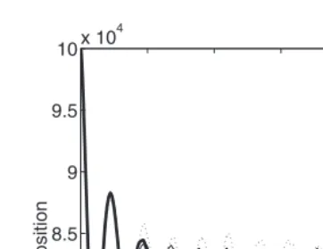
In Fig. 1, we have taken R=4 and investigated the thermodynamic limit by considering increasing values of M from 10000 to 100000. From Fig. 1, we conclude that for t < 30 · 105_{, the thermodynamic limit for the piston is} reached when M > 50000. Other simulations with fixed R ranging from 0.1

(26)

0 5 10 15 20 25 30 35 7 7.5 8 8.5 9 9.5 10x 10 4 time position x 105 a b c d 8.35

Fig. 1. Thermodynamic limit. Position of the piston in function of time fixed for R= N¯ /M=4 and (a) M=10000, (b) M=25000, (c) M=50000, and (d) M=100000. Predicted mechanical equilibrium for adiabatic piston Xf=8.42 · 104. Thermal equilibrium for

conducting piston Xth=30 · 104.

to 300 confirm this result: for t < 30 · 105_{, the evolution corresponds to the} thermodynamic limit if M > 50000.

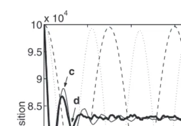
In Figs. 2 and 3, we have considered the time evolution for the piston for different values of R, and values of M such that the evolution corre-sponds to the thermodynamic limit. The simulations (Fig. 2) show that the evolution is very weakly damped for R < 1 and strongly damped for R > 4 in agreement with the conclusion of Section 5. Moreover the piston evolves toward the equilibrium position Xf58.35 · 104, which is in excellent agreement with the predicted value Xf=8.42 · 104obtained from the result of Section 5, i.e., Eq. (139).

The weakly damped oscillations have a period which is in very good agreement with the expected values of Section 5 (see Table I), but the damping coefficient computed over more than 1000 oscillations gives a value several order of magnitude smaller than l given by Eq. (139). For

example for R=0.2, M=100000, we observe a damping equal to 3 · 10−5_l. The oscillations occur around the equilibrium position Xf, and their period remains constant in time (at least up to t=7000 · 105_{which corresponds to}

1500 oscillations and is the time the simulation has been running). As

pre-dicted, the frequency of the oscillations increases with R, but is indepen-dent of M for sufficiently large M. The fluctuations on the amplitude of these oscillations is of order 1%.

(27)

0 5 10 15 20 25 30 6.5 7 7.5 8 8.5 9 9.5 10x 10 4 time position x 105 a _b c d 8.35

Fig. 2. From weak to strong damping. Position of the piston in function of time. (a) R=0.1 and M=100000, (b) R=0.2 and M=100000, (c) R=4 and M=100000, and (d) R=10 and M=30000.

On the other hand for R > 10 and M > 6000, i.e., for strongly damped evolution, it is seen on Fig. 3 that the evolution is independent of R and M if t < 20 · 105_{. We also notice (Fig. 3) that for R > 10, the piston acquires} almost immediately a velocity:

V₁=−0.34 (143) 0 5 10 15 7.5 8 8.5 9 9.5 10x 10 4 time position t 1 x 10 5 a d b c 8.35

Fig. 3. Strong damping. Position of the piston in function of time. (a) R=50 and M=6000, (b) R=50 and M=10000, (c) R=100 and M=4000, and (d) R=100 and M=6000.

(28)

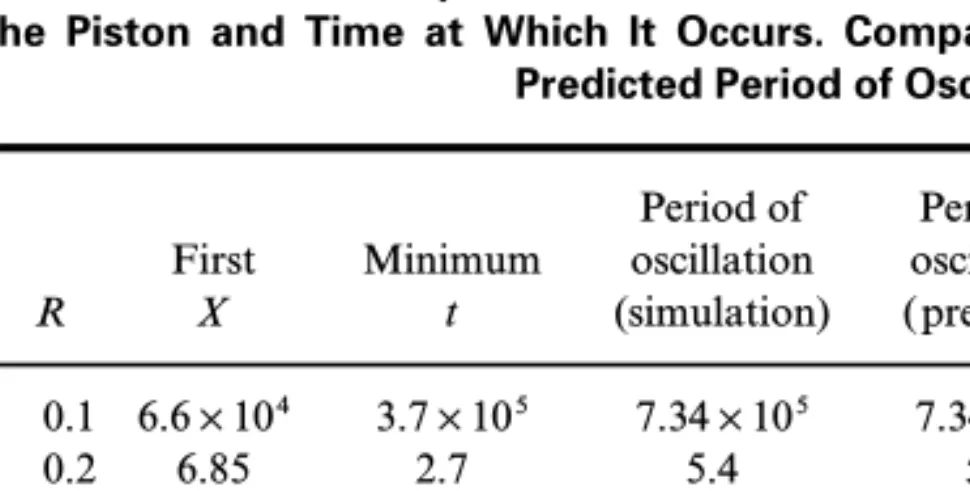
Table I. From Weak to Strong Damping. Simulations with M Sufficiently Large to Describe the Thermodynamic Limit. Value of the First Minimum of the Position of the Piston and Time at Which It Occurs. Comparison Between the Observed and

Predicted Period of Oscillations

Period of Period of Period of

First Minimum oscillation oscillation Oscillation R X t (simulation) ( predicted) at t=30 × 105_(simulation)

0.1 6.6 × 104 _{3.7 × 10}5 _{7.34 × 10}5 _{7.34 × 10}5 _{7.34 × 10}5 0.2 6.85 2.7 5.4 5.29 5.4 1 7.1 1.45 2.94 2.85 2.94 2 7.2 1.20 2.6 3.05 4 7.4 1.0 2.2 5 7.4 0.95 2.1 10 7.5 0.96 2.0 50 7.6 0.9 100 7.6 0.9 200 7.6 0.9 300 7.6 0.9

which is in perfect agreement with V¯ computed above with Eq. (134). Therefore for strong damping the friction coefficient coincide with the computed value during the initial evolution, i.e., as long as the influence of the boundaries (x=0, x=L) did not appear. The piston then arrives at its first minimum position at the time t1=0.9 · 105, which corresponds to the time t−_{for the sound wave to return on the piston, Eq. (135), and reaches} the position of mechanical equilibrium after two oscillations, i.e., at a time

t which is about 4t1 (see also Fig. 4). It is seen on Figs. 1 and 2 that for R between 4 and 10 new oscillations appear after a time of the order 20t1with amplitudedX/L % 4 · 10−3 _{and period approximately equal to 2t}

1 indepen-dent of R and M ( for M large). The amplitude of these new oscillations is modulated with a period about 20t1 and they tend to disappear with time. We are led to conjecture that these oscillations are associated with sound waves propagating in the gases. As we have checked, these oscillations reflect the fact that the velocity distributions of the gases are not Maxwellian. They will be responsible for the approach to Maxwellian dis-tributions. Similar results and conclusions have been obtained in ref. 19. For larger values of R (e.g., R=50 or 100 as shown in Fig. 3) the number of particles necessary to observe the adiabatic evolution over a time interval

40t1is several millions. These simulations would need a very large computer time and have not been conducted.

(29)

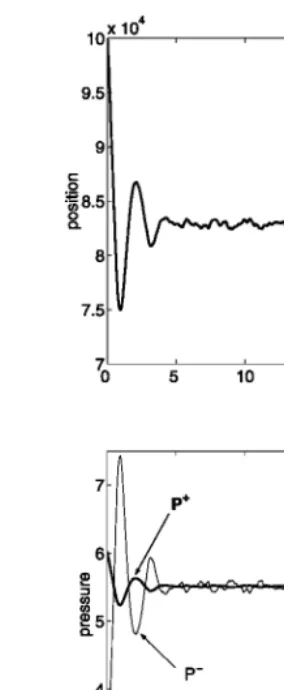
Fig. 4. Adiabatic evolution: Approach to mechanical equilibrium for R=10 and M= 30000. (a) Position, (b) pressure, and (c) temperature. The predicted value for the mechanical equilibrium are Xf=8.42 · 104, p−f=p+f=5.5, T−f=1.54, T+f=9.46.

(30)

In Fig. 4, we show the time evolution for the temperature T± _{of the} gas and for the pressure p±_{defined by}

p−_(t)=N¯ kBT−(t)

X(t) p

+_(t)=N¯ kBT+(t)

(L − X)(t) (144)

where T±_=2E±_/N_{¯ k}

B, E± being the energies of the two compartments. It is seen that these evolutions follow the evolution of the piston. Moreover, we notice that the temperature increases (resp. decreases) under compres-sion (resp. expancompres-sion) of the gas, which reflects the fact that the evolution is adiabatic. We recall that the area A does not play any role. From Fig. 4, we obtain the numerical values for temperatures and pressure when mechanical equilibrium is reached,

T−

f=1.52, T

+

f=9.48, p−=p+=5.5 (145)

which are again in perfect agreement with the expected values (136)–(138)

T−

f=1.54, T+f=9.46, pf=5.5 since N¯ =300000.

Finally from (106) and (107), we have for the change in entropy between the initial and final states:

DS−_=N¯ k

B23 · 10−3 (146)

DS+_=N¯ k

B6.7 · 10−3 (147)

We thus observe numerically an increase in entropy for both gases which once more confirms the adiabatic property of the piston. The result observed in Fig. 3 that for R > 10 the evolution is independent of R leads us to the following

Conjecture. In the thermodynamic limit, the evolution for R Q . is given by the solution of:

(“t+v “x) r−(x, v; t)=d(x) vr−(0, v; t)

+d(x − X(t)) [V(t) − v] r−_{(X(t), v; t)}

(“t+v “y) r+( y, v; t)= − d( y − L) v r+(L, v; t)

− d( y − X(t)) [V(t) − v] r+_{(X(t), v; t)}

where d

dtX=V(t) and V(t) is the solution of

F . V(t)dv r −_{(X(t), v; t)(v − V(t))}2_=FV(t) −. dv r +_{(X(t), v; t)(v − V(t))}2 ₍₁₄₈₎

(31)

This conjecture follows from (65)–(68), with the left boundary placed at the origin (x=0), and the boundary condition at x=X(t)

r±_{(X(t), v; t)=r}±_{(X(t), 2V(t) − v; t)} _for _{v Z V(t)}

which is expected to hold in the thermodynamic limit.(15)

7. CONCLUSIONS

As mentioned in the introduction, we have shown that in the thermo-dynamic limit for the piston (A Q . with N±_{/A, M/A, and L fixed) the} evolution of the piston is deterministic, i.e., the distribution function is

Y(X, V; t)=d(X − Xt) d(V − Vt) where X(t) is the solution of a system of autonomous equations coupled to the one-particle distributions for the gases. Moreover we have shown that in this limit the two-point correlation function for one left (right) particle with the piston factorizes as the product of the individual distribution functions. Furthermore, the evolu-tion is strictly adiabatic ( for M=.) in the sense that the changes in energy are entirely due to work, no heat transfer is involved and the entropy of both gases are strictly increasing. If the length of the cylinder is infinite (and M=.), the piston evolves towards a stationary equilibrium state with velocity V¯ approximately proportional to (p+_{− p}−_{). Therefore, in the} thermodynamic limit (and L=.) the stationary state is a state of mechan-ical equilibrium, iff p+_=p−_.

If the length of the cylinder is finite, we have introduced an assump-tion to express the density of particles and the temperature at the surfaces of the piston by their average values in the left and right compartments. With this assumption, we were able to analyze the evolution and the final state. The numerical simulations, as well as the analytical expressions, have shown that for finite L the motion is characterized by damped oscillations. It is weakly damped if N/M is small and strongly damped if N/M is large. Moreover the numerical values obtained in the simulations confirm all the conclusions derived from the average assumption, except for the damping oscillations which appears a lot smaller than predicted. We are thus led to the conjecture that there are two different mechanisms responsible for fric-tion. One mechanism correctly described by the discussion of Section 4 is associated with the motion of the piston in the absence of recollision (L=.) and is responsible for the stationary state in the infinite cylinder. Another mechanism which is responsible for the damping of oscillations appears to be associated with sound waves, i.e., inhomogeneities in the gases, traveling back and forth between the piston and boundaries. Finally we have observed that over a time interval of order M the evolution is

(32)

independent of N/M, as soon as N/M is large enough. It remains however to give a proof of the result without introducing the average assumption.

In a forthcoming paper, we shall present numerical simulations which show the key difference between the infinite-mass and the finite-mass problems.(20) _{For the finite-mass case, we have the following picture. In a}

first stage, characterised by a time scale of order y1=L `M/E0, the motion of the piston is adiabatic (no heat transfer) and corresponds to the motion that we have described in the thermodynamic limit: it is determi-nistic, with either weak or strong damping, temperature increases under compression; the evolution is independent of M ( for M large enough) and it proceeds until mechanical equilibrium p+_=p−_{is reached. In the second} stage, which is now characterised by a time scale of ordery2=My1/m, the evolution has exactly the opposite properties: it is stochastic, which implies heat transfer through the piston, and the system evolves with constant pres-sure, i.e., p±_(t)=p

f+O(1/M), to a state of thermal equilibrium (T−=T+); in this second stage the evolution depends strongly on M, more precisely we observe the scaling relation XM(t)=X(t/M) where X(t) is independent of N±_{and M.}

ACKNOWLEDGMENTS

The authors are grateful to J. L. Lebowitz, J. Piasecki and Ya. Sinai for stimulating informations about their own work on a similar model. Ch. Gruber is grateful to J. L. Lebowitz for his suggestion to study the thermodynamic limit. He would like to thank J. R. Dorfmann for his friendly invitation where this work was started and the many discussions on Liouville equations with movable boundary conditions. He is also grateful to Ya. Sinai for his numerous e-mails on the problem, his warm hospitality in Princeton, and his constructive criticisms, together with J. L. Lebowitz, concerning the Boltzmann approach previously considered. A. Lesne greatly acknowledges the hospitality at the Institute of Theoreti-cal Physics of the École Polytechnique Fédérale de Lausanne where a part of this research has been performed.

REFERENCES

1. H. B. Callen, Thermodynamics (Wiley, New York, 1963), Appendix C. See also H. B. Callen, Thermodynamics and Thermostatics, 2nd ed. (Wiley, New York, 1985), pp. 51 and 53.

2. Ch. Gruber, Thermodynamics of systems with internal adiabatic constraints: Time evolu-tion of the adiabatic piston, European J. Phys. 20:259–266 (1999).

3. C. Garrod and M. Rosinia, Three interesting problems in statistical mechanics, Amer. J. Phys. 67:1140–1244 (1999).

(33)

4. A. L. Clark and L. Katz, Can. J. Res. A 18:23–63 (1940).

5. Ch. Gruber and J. Piasecki, Stationary motion of the adiabatic piston, Phys. A 268: 258–265 (1999).

6. S. Pache, Propriétés hors-équilibre d’une paroi adiabatique, Diploma work EPFL (2000), unpublished.

7. Ch. Gruber and L. Frachebourg, On the adiabatic properties of a stochastic adiabatic wall: Evolution, stationary non-equilibrium and equilibrium states, Phys. A 272:392–428 (1999).

8. Ya. G. Sinai, Dynamics of a heavy particle surrounded by a finite number of light particles, Theoret. and Math. Phys. 121:1351–1357 (1999).

9. E. Kestemont, C. Van den Broeck, and M. Malek Mansour, The ‘‘adiabatic’’ piston: And yet it moves, European J. Phys. 49:143–149 (2000).

10. J. L. Lebowitz, Stationary non-equilibrium Gibbsian ensembles, Phys. Rev. 114:1192 (1959).

11. J. Piasecki and Ch. Gruber, From the adiabatic piston to macroscopic motion induced by fluctuations, Phys. A 265:463–472 (1999).

12. J. Piasecki and Ya. G. Sinai, A Model of Non-Equilibrium Statistical Mechanics, Proceed-ings from NASI Dynamics: Models and kinetic methods for non-equilibrium many-body systems (Leiden, 1998, Kluwer, 2000).

13. J. Piasecki, Drift velocity induced by collisions, J. Stat. Phys. 104:1145 (2001).

14. V. Balakrishnan, I. Bena, and C. van der Broeck, Diffusion and Velocity Correlation Function in a One-Dimensional System ( preprint 2001).

15. J. L. Lebowitz, J. Piasecki, and Ya. Sinai, in Hard Ball Systems and the Lorentz Gas, D. Szász, ed., Encyclopedia of Mathematical Sciences Series, Vol. 101 (Springer-Verlag, Berlin 2000), pp. 217–227.

16. J. L. Lebowitz, private communication.

17. L. D. Landau and E. M. Lifshitz, Fluid Mechanics (Pergamon Press, 1959), (§ 92). 18. O. L. de Lange and J. Pierruis, Amer. J. Phys. 68:265–270 (2000).

19. N. Chernov and J. L. Lebowitz, Dynamics of a Massive Piston in an Ideal Gas: Oscillatory Motion and Approach to Equilibrium, preprint 2001.

20. Ch. Gruber, S. Pache, and A. Lesne, Finite-size effects in the motion of a massive piston in an ideal gas: Fluctuations and relaxation towards equilibrium, to appear in J. Stat. Phys.