Multiscale, multiphysic modeling of the skeletal muscle during isometric contraction

HAL Id: tel-02067013

https://tel.archives-ouvertes.fr/tel-02067013

Submitted on 13 Mar 2019

HAL is a multi-disciplinary open access archive for the deposit and dissemination of sci-entific research documents, whether they are pub-lished or not. The documents may come from teaching and research institutions in France or abroad, or from public or private research centers.

L’archive ouverte pluridisciplinaire HAL, est destinée au dépôt et à la diffusion de documents scientifiques de niveau recherche, publiés ou non, émanant des établissements d’enseignement et de recherche français ou étrangers, des laboratoires publics ou privés.

during isometric contraction

Vincent Carriou

To cite this version:

Vincent Carriou. Multiscale, multiphysic modeling of the skeletal muscle during isometric contraction. Biomechanics [physics.med-ph]. Université de Technologie de Compiègne, 2017. English. �NNT : 2017COMP2376�. �tel-02067013�

Thèse présentée

pour l’obtention du grade

de Docteur de l’UTC

Soutenue le 4 octobre 2017

Spécialité : Biomécanique et Bio-ingénierie : Unité de

Recherche Biomécanique et Bio-ingénierie (UMR-7338)

Université de Technologie de  Compiègne  Ecole Doctorale  15 Rue Roger Couttolenc  60200 Compiègne   

Multiscale, multiphysic modeling of the 

skeletal muscle during isometric contraction 

 

Thesis Presented to 

 

Sorbonne  University,  Université  de Technologie de  Compiègne Doctoral 

school « Sciences pour l’ingénieur » for the Degree of 

Doctor in Biomechanics and Bioengineering

  Presented and publicly defended by:  4 october 2017  Spécialité : Biomécanique et Bio‐ingénierie 

CARRIOU Vincent

  Jury members :   Reviewers:  Pr. Dario Farina, Professor, Imperial College London, Department of Bioengineering Dr.  Alfredo I. Hernandez, Research Director INSERM, Université de Rennes 1, LTSI  Examiners:  Pr. Catherine Marque, Professor, Université de Technologie de Compiegne, BMBI Dr. David  Guiraud, Research Director INRIA, University of Montpellier 2, LIRMM  Supervisors:  Dr. Sofiane Boudaoud, Associate Professor, Université de Technologie de Compiègne, BMBI  Dr. Jérémy Laforêt, Research Engineer CNRS, Université de Technologie de Compiègne, BMBI 

Ce travail a été réalisé dans le cadre du Labex MS2T. Il a été supporté par le gouvernement français, à travers le "Programme Investissement pour l’Avenir" encadré par l’Agence Nationale pour la Recherche (Reference ANR-11-IDEX-0004-02).

Dans un premier temps, je tiens à remercier Prof. Marie-Christine Ho Ba Tho, direc-trice du laboratoire BMBI et Dr. Karim El Kirat, maître de conférence au laboratoire BMBI et responsable du Master MS2C, pour m’avoir donné l’opportunité de réaliser cette thèse dans le laboratoire BMBI. Je tiens aussi à remercier Prof. Catherine Marque, re-sponsable de l’équipe NSE du laboratoire BMBI dans laquelle j’ai réalisé ma thèse, pour son soutien et ses encouragements indéfectibles tout au long de cette thèse ainsi que pour l’ensemble de ses conseils avisés qu’elle a su me donner au bon moment.

Merci aux membres du jury, Prof. Dario Farina, Prof. Alfredo I. Hernandez, Prof. Catherine Marque, Dr. Guiraud David qui ont trouvé du temps et ont fait le déplacement pour assister à la soutenance de thèse malgré leur emploi du temps chargé.

Un grand merci à mes directeurs de thèse, Dr. Sofiane Boudaoud et Dr. Jérémy Laforêt pour m’avoir fait confiance durant la thèse. J’aurai énormément appris professionellement et personnelement auprès d’eux. Merci pour leur investissement constant et sans faille durant ces 3 années. Ils ont su m’insuffler une excellente dynamique pour tirer le maximum de mon potentiel. Merci Dr. Sofiane Boudaoud pour ces réunions enflammées nourries par ton dynamisme, ta vision et tes idées avant gardistes du domaine, ta rigueur, ta motivation omniprésente et ta bienveillance. Merci pour toujours avoir cru en moi et en ce que l’on faisait, merci pour m’avoir constamment encouragé même dans les moments plus difficiles. Merci Dr. Jérémy Lafôret pour ces longues heures de discussion et de réflexion autour de ma thèse ou de sujets diverses. Merci pour m’avoir transmis tes connaissances, ta culture et ta curiosité qui sont sans limites. Merci d’avoir toujours pris le temps de m’écouter et d’avoir toujours eu les mots exacts aux bons moments. Je vous aurai bien embêté durant ces 3 années mais nous avons formé une excellente équipe et fourni du très bon travail. Ça aura été difficile mais en regardant en arrière, ça en valait le coup.

De plus, merci à l’ensemble des membres du laboratoire BMBI et de l’UTC plus glob-alement : Adrien Letocart, Dr. Firas Farhat, Dr. Noujoude Nader, Kevin Lepetit, Saeed Zahran, Dr. Malek Kammoun, Quentin Demigny, Dr. Redouane Ternifi, Dr. Francis Canon, Dr. Didier Gamet, Dr. Jean-François Grosset, Dr. Khalil Ben Mansour, Lilandra Boulais et Megane Beldjilali Labro. Merci pour ces moments dont je me souviendrai toute ma vie et merci pour ces discussions/collaborations scientifiques que nous avons pu avoir. Un merci tout particulier à mes parents Nelly et Jean-René qui m’ont toujours soutenu depuis le début. Merci pour votre soutien sans faille et votre amour continue. Si j’en suis ici aujourd’hui, c’est en grande partie grâce à eux. Merci à Marine et Dominique, ma soeur et mon frère, pour vos encouragements et ces moments passés ensemble qui m’ont permis de me déconnecter et de décompresser. Merci à mes amis que je considère comme des membres de ma famille, Ludovic, Soraya, Nour, Côme, Laéticia et Véronique pour

Avant propos

: Les systèmes neuromusculaire et musculosquelettique sont des systèmes de systèmes complexes qui interagissent parfaitement entre eux afin de produire le mouvemement. En y regardant de plus près, ce mouvement est la résultante d’une force musculaire créée à partir d’une activation du muscle par le système nerveux centrale. En parallèle de cette activité mécanique, le muscle produit aussi une activité électrique elle aussi contrôlée par la même activation. Cette activité électrique peut être mesurée à la surface de la peau à l’aide d’électrode, ce signal enregistré par l’électrode se nomme le signal Electromyogramme de surface (sEMG). Comprendre comment ces résultats de l’activation du muscle sont générés est primordiale en biomécanique ou pour des applica-tions cliniques. Evaluer and quantifier ces interacapplica-tions intervenant durant la contraction musculaire est difficile et complexe à étudier dans des conditions expérimentales. Par conséquent, il est nécessaire de développer un moyen pour pouvoir décrire et estimater ces interactions. Dans la littérature de la bioingénierie, plusieurs modèles de génération de signaux sEMG et de force ont été publiés. Ces modèles sont principalment utilisés pour décrire une partie des résultats de la contraction musculaire. Ces modèles souffrent de plusieurs limites telles que le manque de réalisme physiologique, la personnalisation des paramètres, ou la représentativité lorsqu’un muscle complet est considéré. Dans ce tra-vail de thèse, nous nous proposons de développer un modèle biofidèle, personnalisable et rapide décrivant l’activité électrique et mécanique du muscle en contraction isométrique. Pour se faire, nous proposons d’abord un modèle décrivant l’activité électrique du muscle à la surfac de la peau. Cette activité électrique sera commandé par une commande volon-taire venant du système nerveux périphérique, qui va activer les fibres musculaires qui vont alors dépolariser leur membrane. Cette dépolarisation sera alors filtrée par le volume conducteur afin d’obtenir l’activité électrique à la surface de la peau. Une fois cette activ-ité obtenue, le système d’enregistrement décrivant une grille d’électrode à haute densactiv-ité (HD-sEMG) est modélisée à la surface de la peau afin d’obtenir les signaux sEMG à partir d’une intégration surfacique sous le domaine de l’électrode. Dans ce modèle de généra-tion de l’activité électrique, le membre est considéré cylindrique et multi couches avec la considération des tissues musculaire, adipeux et la peau. Par la suite, nous proposons un modèle mécanique du muscle décrit à l’échelle de l’Unité Motrice (UM). L’ensemble des résultats mécanique de la contraction musculaire (force, raideur et déformation) sont déterminées à partir de la même commande excitatrice du système nerveux périphérique. Ce modèle est basé sur le modèle de coulissement des filaments d’actine-myosine proposé par Huxley que l’on modélise à l’échelle UM en utilisant la théorie des moments utilisée par Zahalak. Ce modèle mécanique est validé avec un profil de force enregistré sur un sujet paraplégique avec un implant de stimulation neurale. Finalement, nous proposons aussi trois applications des modèles proposés afin d’illustrer leurs fiabilité ainsi que leurs utilité. Tout d’abord une analyse de sensibilité globale des paramètres de la grille HD-sEMG est présentée. Puis, nous présenterons un travail fait en collaboration avec une autre doctorante une nouvelle étude plus précise sur la modélisation de la relation HD-sEMG/force en personnalisant les paramètres afin de mimer au mieux le comportement du Biceps Brachii. Pour conclure, nous proposons un dernier modèle quasi-dynamique décrivant l’activité électro-mécanique du muscle en contraction isométrique. Ce modèle déformable va actualiser l’anatomie cylindrique du membre sous une hypothèse isovolu-mique du muscle.

Mots-clés

: Système de systèmes; modélisation; contraction du muscle squelettique; activité électrique; activité mécanique; optimisation; modèle couplé; analyse de sensibilité; relation sEMG/force

Abstract

: The neuromuscular and musculoskeletal systems are complex System of Systems (SoS) that perfectly interact to provide motion. From this interaction, a muscular force is generated from the muscle activation commanded by the Central Nervous System (CNS) that pilots joint motion. In parallel an electrical activity of the muscle is generated driven by the same command of the CNS. This electrical activity can be measured at the skin surface using electrodes, namely the surface electromyogram (sEMG). The knowl-edge of how these muscle outcomes are generated is highly important in biomechanical and clinical applications. Evaluating and quantifying the interactions arising during the muscle activation are hard and complex to investigate in experimental conditions. There-fore, it is necessary to develop a way to describe and estimate it. In the bioengineering literature, several models of the sEMG and the force generation are provided. They are principally used to describe subparts of the muscular outcomes. These models suffer from several important limitations such lacks of physiological realism, personalization, and rep-resentability when a complete muscle is considered. In this work, we propose to construct bioreliable, personalized and fast models describing electrical and mechanical activities of the muscle during contraction. For this purpose, we first propose a model describing the electrical activity at the skin surface of the muscle where this electrical activity is deter-mined from a voluntary command of the Peripheral Nervous System (PNS), activating the muscle fibers that generate a depolarization of their membrane that is filtered by the limb volume. Once this electrical activity is computed, the recording system, i.e. the High Density sEMG (HD-sEMG) grid is defined over the skin where the sEMG signals is deter-mined as a numerical integration of the electrical activity under the electrode area. In this model, the limb is considered as a multilayered cylinder where muscle, adipose and skin tissues are described. Therefore, we propose a mechanical model described at the Motor Unit (MU) scale. The mechanical outcomes (muscle force, stiffness and deformation) are determined from the same voluntary command of the PNS, and is based on the Huxley sliding filaments model upscale at the MU scale using the distribution-moment theory proposed by Zahalak. This model is validated with force profile recorded from a subject implanted with an electrical stimulation device. Finally, we proposed three applications of the proposed models to illustrate their reliability and usefulness. A global sensitivity analysis of the statistics computed over the sEMG signals according to variation of the sEMG electrode grid is performed. Then, we proposed in collaboration a new HD-sEMG/force relationship, using personalized simulated data of the Biceps Brachii from the electrical model and a Twitch based model to estimate a specific force profile corre-sponding to a specific sEMG sensor network and muscle configuration. To conclude, a deformable electro-mechanical model coupling the two proposed models is proposed. This deformable model updates the limb cylinder anatomy considering isovolumic assumption and respecting incompressible property of the muscle.

Keywords

: System of systems; modeling; skeletal muscle contraction; electrical ac-tivity; mechanical acac-tivity; optimization; coupling model; sensitivity analysis; sEMG/force relationship

drical multilayered muscle model. Biomedical Physics & Engineering Express, 2(6), 2016.

• M. Al Harrach, V. Carriou, S. Boudaoud, J. Laforet, F. Marin. Analysis of the sEMG/Force Relationship using HD-sEMG Technique and Data Fusion: A Simula-tion Study. Computers in Biology and Medicine, 83: 34-47.

• V. Carriou, S. Boudaoud, and J. Laforet. Speedup computation of HD-sEMG signals using a motor unit specific electrical source model. Medical & Biological Engineering & Computing. In review.

• M. Al Harrach, S. Boudaoud, V. Carriou, J. Laforet, A. J., Letocart, J-F. Grosset, and F. Marin. Investigation of the HD-sEMG Probability Density Function Shapes with Varying Muscle Force using Data Fusion and Shape Descriptors. Computers in Biology and Medicine. In review.

• V. Carriou, S. Boudaoud, J. Laforet, A. Mendes, F. Canon, and D. Guiraud. Multiscale modeling of skeletal muscle contractile properties in isometric conditions. Journal of Neural Engineering. Under preparation.

International conference papers:

• V. Carriou, M. Al Harrach, J. Laforet, and S. Boudaoud. Sensitivity Analysis of HD-sEMG Amplitude Descriptors Relative to Grid Parameter Variation. In XIV Mediterranean Conference on Medical and Biological Engineering and Computing, 57: 119–123. Springer International Publishing, 2016.

• V. Carriou, J. Laforet, S. Boudaoud, and M. Al Harrach. Realistic motor unit placement in a cylindrical HD-sEMG generation model. In 2016 38th Annual In-ternational Conference of the IEEE Engineering in Medicine and Biology Society (EMBS), 1704–1707, 2016.

• M. Al Harrach, B. Afsharipour, S. Boudaoud, V. Carriou, F. Marin and R. Mer-letti. Extraction of the Brachialis muscle activity using HD-sEMG technique and Canonical Correlation Analysis. In 2016 38th Annual International Conference of the IEEE Engineering in Medicine and Biology Society (EMBS), 2378-2381, 2016. • R. El Koury, V. Carriou, S. Boudaoud, J. Laforet, and A. Diab. Precise Assessment

of HD-sEMG Grid Misalignment Using Nonlinear Correlation. In 4th International Conference on Advances in BioMedical Engineering (ICABME). Accepted.

• V. Carriou, J. Laforet, and S. Boudaoud. Object-oriented programming of opti-mized analytic neuromuscular model. In 7th International Conference on Compu-tational Bioengineering (ICCB). Accepted.

Body Mass Indicator BMI

Brachialis BR

Central Nervous System CNS

Coefficient of Variation CoV

Design Of Experiment DOE

Electrical Stimulation ES

Electromyogram EMG

Elementary Effect EE

Elementary Effect Method EEM

Electroencephalogram EEG

Fast Fatigable FF

Fast Fatigable MU FFMU

Fast Intermediate FI

Fast Intermediate MU FIMU

Fast Resistant FR

Fast Resistant MU FRMU

Fiber Action Potential FAP

Finite Element Method FEM

Functional Electrical Stimulation FES

Hermite Rodriguez HR

High Density HD

High Density sEMG HD-sEMG

High Recruitment Strategy HRS

High order Statistics HOS

Human Machine Interface HMI

Inter Spike Intervals ISI

Intracellular Action Potential IAP IntraClass Correlation ICC

Low Recruitment strategy LRS Magnetic Resonance Imaging MRI Maximal Voluntary Contraction MVC

Motor Unit MU

MU Action Potential MUAP

MyoTendinous Zone MTZ

Neural Electrical Stimulation NES

Neuromuscular Junction NMJ

Non Propagating Component NPC

Normalized-Root-Mean-Square-Error NRMSE Ordinary Differential Equations ODEs

Peak firing rate PFR

Peripheral Nervous System PNS

Power Spectral Density PSD

Probability Density Function PDF Recruitment Threshold Excitation RTE

Rectus Femoris RF

Root Mean Square RMS

Sarcosplasmic Reticulum SR

Single Fiber action potential SFAP

Slow S

Sensitivity Index SI

Slow MU SMU

Standard Deviation std

surface ElectroMyoGram sEMG

System of Systems SoS

Vastus intermedius VI

Vastus lateralis VL

1 State of the art and problematic 5

1.1 Introduction . . . 6

1.2 The neuro-musculo-skeletal system . . . 7

1.2.1 Motion genesis . . . 8

1.3 The neuro-muscular system . . . 9

1.3.1 The peripheral neural system . . . 9

1.3.2 Skeletal muscle . . . 12

1.3.3 Muscle contraction . . . 16

1.4 Surface electromyography . . . 20

1.4.1 Electrode configurations and spatial filtering . . . 21

1.4.2 High Density sEMG (HD-sEMG) technique . . . 22

1.5 Modeling of the neuromuscular system . . . 23

1.5.1 MU recruitment scheme models . . . 23

1.5.2 Electrical models . . . 25

1.5.3 Mechanical models . . . 30

1.5.4 Multi-physic models . . . 35

1.5.5 Summary . . . 37

1.6 Objectives of the thesis . . . 38

2 Modeling the muscle electrical activity 41 2.1 Introduction . . . 43

2.2 Fast generation model of HD-sEMG signals . . . 44

2.2.1 Overview of the model geometry and computation . . . 44

2.2.2 Modeling the MU recruitment scheme . . . 46

2.2.3 Fiber electrical source modeling . . . 47

2.2.4 Computation of the transfer function of a multilayer cylindrical vol-ume conductor . . . 49

2.2.5 Spatial frequency sampling . . . 52

2.2.6 Computing the electrical activity . . . 54

2.2.7 Modeling the recording system and the sEMG signal generation . . 56

2.2.8 Model implementation . . . 58 ix

2.2.9 Simulation results . . . 60

2.3 Discussion . . . 66

2.4 Conclusion . . . 70

2.5 Motor unit electrical source modeling . . . 71

2.5.1 Macro-scale motor unit electrical source . . . 72

2.5.2 Results . . . 77

2.5.3 Discussion . . . 81

2.5.4 Conclusion . . . 82

2.6 Simulating MU realistic placement . . . 83

2.6.1 Unconstrained MU positionning . . . 84

2.6.2 Best Candidate MU positionning . . . 84

2.6.3 Results . . . 86

2.6.4 Conclusion . . . 89

2.7 General conclusion . . . 89

3 Modeling the muscle mechanical activity 91 3.1 Introduction . . . 92

3.2 Model overview . . . 93

3.3 Activation model . . . 93

3.3.1 MU recruitment . . . 94

3.3.2 Modeling the calcium dynamic of the fiber . . . 96

3.3.3 MU activation . . . 97

3.4 Mechanical model of the muscle during isometric contraction . . . 98

3.5 Results . . . 101

3.5.1 Fusion frequency study . . . 102

3.5.2 Motor unit scale . . . 103

3.5.3 Comparison with the twitch model . . . 104

3.5.4 Model validation . . . 106

3.5.5 Voluntary contraction simulation . . . 109

3.6 Discussion . . . 111

3.7 Conclusion . . . 112

4 Applications of the proposed models 115 4.1 Introduction . . . 117

4.2 Global sensitivity analysis . . . 117

4.2.1 Electrode grid recording . . . 118

4.2.2 Global sensitivity analysis . . . 120

4.2.3 Signal features . . . 122

4.2.4 Parameter sensitivity results . . . 122

4.2.5 Discussion & Conclusion . . . 129

4.3 sEMG/force relationship estimation . . . 131

4.3.1 HD-sEMG generation model . . . 133

4.3.2 Muscle force generation model . . . 134

4.3.3 Model personalization using experimental data . . . 135

4.3.4 Simulation procedure . . . 137

4.3.5 Data fusion & HD-sEMG/force relationship fitting . . . 139

4.3.6 Results . . . 140

4.3.7 Discussion & Conclusion . . . 146 4.4 Quasi-dynamic model of the skeletal muscle during isometric contraction . 149

2.5 Configuration of simulation . . . 61

2.6 Related computation time according to the MU type (mean ± std) . . . . 65

2.7 Computation time according to the number of processes used . . . 65

2.8 Anatomical MU parameters . . . 74

2.9 Configuration of simulation . . . 77

2.10 Mean NRMSE between the generated MUAP . . . 77

2.11 NRMSE computed on the signals between the fiber electrical source model and the filtered MU electrical source model, the PSD and the statistics (mean ± std) over the five anatomies at 30, 50 and 70% of the MVC . . . 79

2.12 Computation time for the five anatomies (mean ± std) at 30, 50 and 70% of the MVC for both electrical source models using serial and parallel con-figurations . . . 80

2.13 Radial MU position distribution according to MU type . . . 84

2.14 Configuration of simulation . . . 87

3.1 Fixed parameters . . . 101

3.2 Parameters used for the fusion frequency . . . 102

3.3 Parameters used for the twitch model . . . 105

3.4 Parameters used for the fusion frequency . . . 107

3.5 Parameters used for the fusion frequency . . . 108

4.1 Parameters used for sensitivity analysis and their variation range. . . 122

4.2 Parameters used for the generation of the ten anatomies. . . 123

4.3 Detailed monopolar ARV and RMS features sensitivity for all parameters on the mean features of the ten anatomies. . . 125

4.4 Detailed monopolar kurtosis and skewness features sensitivity for all pa-rameters on the mean features of the ten anatomies. Highlighted values in red correspond to values indicating a non monotonous effect of the parameter.126 4.5 Detailed bipolar ARV and RMS features sensitivity for all parameters on the mean features of the ten anatomies. . . 127

4.6 Detailed bipolar kurtosis and skewness features sensitivity for all parame-ters on the mean features of the ten anatomies. Highlighted values in red correspond to values indicating a non monotonous effect of the parameter. 128 4.7 Detailed laplacian ARV and RMS features sensitivity for all parameters on

the mean features of the ten anatomies. Highlighted values in red corre-spond to values indicating a non monotonous effect of the parameter. . . . 129 4.8 Detailed laplacian kurtosis and skewness features sensitivity for all

param-eters on the mean features of the ten anatomies. Highlighted values in red correspond to values indicating a non monotonous effect of the parameter. 130 4.9 Fixed parameters of the cylindrical HD-sEMG simulation model. . . 133 4.10 Twitch parameters . . . 135 4.11 The measured morphological parameters using ultrasound images for each

subject . . . 137 4.12 MU percentages for each distribution. . . 137 4.13 Morphological parameters used for simulations . . . 139 4.14 The NRMSE computed for the 3rd degree polynom fitting by optimization

for the different morphological, anatomical and neural parameter values in %. . . 144 4.15 Parameters used for the simulations . . . 154

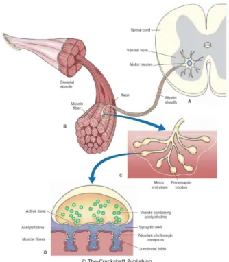
1.4 Description of the PNS and its communication with the muscular system. (A) Cell body of an α-motoneuron. (B) and (C) Myelinated axon inner-vating skeletal fibers. (D) The synaptic description with its vesicles and

ACh. . . 11

1.5 Variety of muscle architecture in the human body. . . 13

1.6 Macroscopic structure of skeletal muscle. . . 13

1.7 Microscopic structure of a skeletal muscle fiber. . . 14

1.8 Anatomic structure of a muscle myofibril. . . 15

1.9 Histochemical appearance of different types of fiber in the Brachialis muscle 15 1.10 The AP of a fiber membrane when a nerve firing arrives. At rest, the tension is at -70 mV. When the pulse arrives, a depolarization occurs rapidly followed by a repolarization of the membrane. This repolarization falls below the voltage at rest, at this time a phenomenon of hyperpolarization intervenes to return potential to the rest tension. (image de c Pearson Prentice Hall, Inc 2005) . . . 17

1.11 The different stages of muscle fiber contraction cycle . . . 18

1.12 General shape of a fiber twitch. . . 19

1.13 Different response of the twitch according to the stimulation time. . . 19

1.14 Example of MU recruitment pattern exhibiting the firing discharge of ev-ery 10th _{MU (Top). The corresponding simulated sEMG signal detected} by bipolar surface electrode according to the recruitment pattern (Mid-dle). The corresponding simulated force according to the same recruitment pattern (Bottom) . . . 20

1.15 Example of an 8×8 HD surface electrode grid placed on the Biceps Brachii muscle (Refa 136, TMSI, Netherlands) . . . 22

1.16 Different rate coding strategies. MU firing rate increases linearly (L) and non-linearly (R) according to the force level increase . . . 25

1.17 Example of the discharge instants (vertical strokes) of every 10th MU in a pool of 120 MUs . . . 25

1.18 Muscle fiber current source density distribution represented by a spatio-temporal function . . . 27

1.19 Volume conductor configuration with adipose layer tissue and finite length of the muscle . . . 27 1.20 Planar volume conductor configuration with skin, adipose tissues and

mus-cle. d is the skin thickness. h1 corresponds to the adipose tissue thickness

and y0 is the depth of the fiber within the muscle . . . 28

1.21 Radial view of the bi-pinnate muscle. The muscle fibers have two orienta-tions defined by angles θ± . . . 29 1.22 Finite element model of the limb with muscle, adipose and skin tissues . . 29 1.23 Rheological Hill model of the skeletal muscle . . . 30 1.24 Force-velocity relationship of a tetanized muscle . . . 31 1.25 Sliding filaments representation. A represents the actin site, M the myosin

site and X the distance between the actin site and the equilibrium site O. . 31 1.26 Dependence of the rate functions f and g according to x. Formation of

linking A and M sites is described by f (reaction 2). Breaking the bridge is described by g (reaction 3) . . . 32 1.27 Muscle model El Makssoud . . . 33 1.28 Calcium definition after an electrical stimulus . . . 34 1.29 Mechanical model including masses and dampers inspired from the Hill–Maxwell

model . . . 34 1.30 Twitch shape according to the MU type . . . 36 1.31 Geometry of the tibialis anterior muscle and the fiber distribution, where

the fibers indicate the local membrane potential in color . . . 37 1.32 Scheme presenting the scheme for generating the electro-mechanical

out-comes of the skeletal muscle during contraction (red box). A MU recruit-ment pattern is defined describing the firing times of each MU composing the muscle (blue box). Then, the mechanical model represented at the MU scale simulated the muscle force as well as its deformation (purple box). This deformation (ε) is considered in the electrical model where the limb is described as a multilayered cylinder. Once the muscle updated according to the deformation, the electrical model will compute the electrical activity of the muscle as the sum of the MUAPs at the skin surface (green box). Finally, the sEMG signals are simulated through a numerical integration of the values on the electrical surface under the electrode definition area. . 40 2.1 Muscle’s electrical activity model scheme computation. . . 44 2.2 (L) Muscle geometry in cylindrical coordinates. (R) Longitudinal

cross-section of the cylinder. R is the radial position of the fiber, ρa, ρb and ρc

are the muscle, fat and skin radius, respectively. . . 45 2.3 Model’s calculus scheme to compute one SFAP. Recruitment represents the

discharge times of the MU in time (t). A Fourier transform (F ) is applied for computing in frequency domain. Source depicted the intracellular ac-tion potential along the longitudinal direcac-tion of the fiber in time when a discharge time is triggered (z, t). A 2D Fourier transform (F2) is applied on it. Transfer function presents the volume conductor transfer function computed according to the composition of the volume conductor in spatial frequency domain (kθ, kz). Electrical activity over the skin surface is finally

computed with a 3D inverse Fourier transform (F−3) and potential map is obtained in the spatio-temporal domain (θ, z, t). . . . 46

concentric-ring electrode shapes. . . 57 2.8 Model implementation block diagram describing the dependencies between

modules. . . 59 2.9 Examples of simulated MUAP and SFAP recorded with 2 different electrode

shapes at different angular and longitudinal positions for a muscle with three layers (muscle, adipose and skin tissues). . . 62 2.10 Defined areas with both electrode definitions. . . 63 2.11 Detection volume for a 1mm electrode radius placed at (θ, z) = (0, 0); color

scale indicates the corresponding amplitude ratio range. . . 64 2.12 Large scale simulation. First contraction represents a high plateau (80 %

MVC) held for 2.5 s of simulation; second contraction describes a ramp on 2 s kept for 1 s (from 0 to 80 % MVC); Last contraction illustrates a low plateau (40 % MVC) helds for 2.5 s. . . . 67 2.13 Two different isobarycenters computed for the MU macro electrical source

model based on the fibers position within the corresponding MU. . . 73 2.14 Example of σM U values according to MU type and MU depth computed by

the described optimization algorithm (optimal) and equation (2.53) (Gaus-sian). Grey boxes define the MU physiological position according to its type (see Table 2.13). Areas in white mean that the MU cannot be physiolog-ically placed at this position for a Biceps Brachii muscle. Even though, simulations were computed on all the possible radial position to study the global trend. . . 76 2.15 Electric time representation of a MU on one position of the spatial electrical

map according to the MU type. In red the signal computed with the fiber electrical source model. In blue the signal computed with the filtered MU electrical source model. In green the signal computed with the MU electrical source model without filtering. . . 78 2.16 sEMG signal observed on a time window (100 ms) and generated at 70%

MVC with the two electrical source models recorded on the same electrode. 80 2.17 Anatomy composed of 300 MUs generated with unconstrained uniform

dis-tribution. . . 85 2.18 Anatomy composed of 300 MUs generated with constrained uniform

dis-tribution. . . 86 2.19 Fiber density by both algorithms and fibers histograms in ρ and θ axis.

Each case is about 0.1681 mm2_{. . . . 88}

2.20 Normalized experimental and simulated RMS values map on the 64 elec-trodes at 70% MVC. . . 88

3.1 Model block diagram. On the left there is the input of the model corre-sponding to the recruitment pattern describing the discharge instant of the recruited MUs. On the right the mechanical model scheme, determining the contribution of each MUs then, processes at the muscle scale in or-der to determine the muscle force (Fc), the muscle stiffness (kc) and its

deformation (εc). . . 94

3.2 Example of simulated voluntary MU recruitment at 30% of the Maximum Voluntary Contraction (MVC) for a muscle composed of 100 MUs with the following MUs distribution type: 33% type I, 33% type IIa, 17% type IIx and 17% type IIb. . . 95 3.3 Example of elicited recruitment where 32.4% of the muscle fibers are

re-cruited for the same muscle as in Fig. 3.2. . . 96 3.4 Calcium dynamic of MU according to its type. The neural AP reaches the

MUs at 0.5s. . . 97 3.5 Muscle activation states α, β and γ according to a voluntary contraction

at 50% MVC. . . 98 3.6 Mechanical rheological model of the muscle, including masses and dampers

with N parallel contractile elements representing the MU . . . . 99 3.7 Fusion frequency evaluation for M1. . . 103

3.8 Fusion frequency evaluation for M2. . . 103

3.9 MU force response to the stimulation frequency according to its type. . . . 104 3.10 Fusion frequency for M2 with twitch model. . . 105

3.11 MU force response to the stimulation frequency according to its type using the twitch model. . . 106 3.12 Normalized generated force in experimental conditions following the

pro-tocol presented above compares to simulated force from the proposed me-chanical muscle model . . . 107 3.13 Cumulative plot representing the force contribution for each muscle

com-posing the quadriceps muscle presented above at the stimulation intensity 1.6mA (corresponding to the fourth stimulation). In blue the VL force contribution, in green the VM force contribution, in red the VI force con-tribution and in cyan the RF force concon-tribution. . . 109 3.14 Force profiles for voluntary contractions from 10 to 100% MVC using the

defined twitch model and the proposed muscle mechanical model. . . 110 3.15 Mean and std computed from both models from 10 to 100% MVC. . . 110 4.1 A 8×8 electrode grid representation with the studied grid parameters. . . . 119 4.2 8×8 electrode grid placed on the surface of the muscle skin. Blue electrode

shows the monopolar arrangement (64 signals). Green electrodes shows the bipolar arrangement with corresponding weight on the electrode (56 sig-nals). Red electrodes sh ows the laplacian arrangement with corresponding weight on the electrode (36 signals). . . 119 4.3 Elementary Effect (EE) computation diagram. X_i1and X_i2are two different

values of the parameter Xi. X

(1)

∼i and X (2)

∼i are two different parameter sets

excluding parameter Xi. EE(Xi(j)) is the Elementary Effect of the tested

parameter X_i(j) value with the jth value of the parameter set. X_i(1)X(1)_∼i corresponds to one set of parameter, X_i(2)X(1)_∼i is equivalent to the same set of parameter with a different value of the parameter Xi. . . 121

4.7 Parameters ranking according to the features for laplacian arrangement on the grid. . . 128 4.8 The cylindrical limb model and HD-sEMG grid. . . 134 4.9 The three ultrasound images of the BB muscle taken for the extraction of

morphological parameters for one of the subjects. . . 136 4.10 The profiles of recruitment threshold with respect to the MUS for the LRS

and HRS. . . 138 4.11 Schematic diagram presenting the configurations of parameters used for the

different simulations where Sim defines the different morphological values defined in Table 4.13. . . 138 4.12 The HD-sEMG/force relations for the five anatomies relative to different

morphological parameters. . . 141 4.13 The HD-sEMG/force relations for the five anatomies relative to anatomical

and neural parameters (see Table 4.12) with the points indicated on the curves are the inflection points). . . 142 4.14 The variation of the evaluation values with respect to the fitting type. . . . 143 4.15 P3, P2 and P1 coefficients variation according to adipose tissue thickness

value for the five anatomies. . . 145 4.16 P3, P2 and P1 coefficients variation according to skin tissue thickness value

for the five anatomies. . . 145 4.17 P3, P2 and P1 coefficients variation according to the different MU type

distributions for the five anatomies. . . 146 4.18 P3, P2 and P1 coefficients variation according to the different spatial

re-cruitment strategies (LRS vs HRS) and firing rates ( linear vs nonlinear) for the five anatomies. . . 147 4.19 Computation scheme of the deformable model. Formerly, both

mechan-ical and electrmechan-ical models performed the simulations without interacting together (opaque red lines). Currently, the deformable model simulation is performed first and communicate the corresponding muscle deformation according to the MU recruitment pattern. This deformation will be consid-ered to shorten the cylindrical muscle volume under isovolumic assumption (plain red lines). . . 150 4.20 Determination of the muscle shortening during the isometric contraction. . 151 4.21 Illustration of the anatomical changes in the of the muscle between the non

deformed model and the deformed. . . 152 4.22 Geometrical muscle shortening (bottom) and muscle swelling (top)

accord-ing to four contraction levels: 10, 30, 70, 100% MVC. In red the muscle and in blue the representative tendons. . . 155

4.23 Muscle shortening and swelling relationship according to contraction levels. The red dots exhibits the values of the corresponding effect for the given activation. In red the linear relationship. . . 155 4.24 Stress-strain curve. Red dots are the values computed for each contraction

level. Blue line is the linear regression function computed according the to red dots. . . 156 4.25 sEMG signal on a frame of 100ms recorded from the same electrode from

two simulations where the deformation is considered (green) and isn’t (blue).157 4.26 Mean ± std (%) NRMSE computed for the 5 anatomies over the 64 signals

according to the muscle contraction level. . . 158 4.27 Mean ± std NRMSE (mean and std) computed between the amplitude

statistics from the non deformable model and the deformable according to contraction level for the five anatomies. . . 159

Yet, movement is crucial for survival and human life, thus it is imperative to understand all its aspects that can determine the functions and detect anomalies of the musculoskele-tal and neuromuscular systems [3]. Accordingly, the neuromuscular and musculoskelemusculoskele-tal systems can be evaluated along with the diagnosis and management of both neurological and orthopedic diseases through estimation and qualification of this mechanical response which is the force [4]. However, as mentioned earlier, the muscle activation have another response that is correlated to the mechanical one; the electrical activity. This electrical response is called the Electromyogram (EMG) and can be measured in a non invasive manner at the skin surface using surface electrodes [2].

These two phenomena occuring during the contraction of the muscle are the outcomes of complex microscopic interactions. During muscular pathologies one or several of these interactions are disrupted inducing serious consequences on the contractile responses. Considering the complex underlying interactions arising during the muscle contraction these disruptions are hardly diagnosed. For these reasons, bioreliable modeling of the skeletal muscle during contraction is one of the leading challenges in biomechanics and motor control. Bioreliable models can accurately describe the mechanisms controling the muscle activation. Moreover, major interest in such models is the possibility to know all the variables involved during the phenomenon. During experimental protocols studying the muscle contraction, some properties of the muscle cannot be known and thus, may be different among the subjects. These different properties can lead to misinterpret the results of the study. In order to reduce this error due to inter-variability of the muscle composition the number of subjects for this study must be important leading to expen-sive and long study. Using such a model can reduce this inter-variability since all the parameters physiologically representing the skeletal muscle are controlled by the user.

Understanding the muscle contraction and how these phenomena are created, is funda-mental in many areas such as the study of joints and body motion. Moreover this possible new knowledge can help practitioners with diagnosis or development of new treatments. In this thesis we will propose three models describing, the electrical activity of the muscle, the mechanical activity of the muscle and a deformable electro-mechanical activity of the muscle during isometric, isotonic and anisotonic non fatiguing contractions. Since the beginning of the 21st _{century, computational power significantly increased leading to the}

possibility to perform large and precise simulations or complex data processing using a classical workstation. Following this drift, use of high-level programming language by the scientific community emerges. Stimulating by the scientific community, a large ecosystem of generic methods in several research fields (image and signal processing, multi-domain dynamic systems dynamic, multi-channel processing, linear algebra computation, etc.) is developed and accessible. For this purpose, the proposed models are developed in Python programming language, providing access to several scientific libraries that allow an opti-mized programming that will minimize the computation time of the models. Based on all of the above, this manuscript is organized as follow:

• Chapter 1: in this chapter, we will introduce the main notions concerning the neuro-muscular system and motion genesis, essentially the skeletal muscle properties and architecture, the Motor Unit (MU) and the fiber types. Wherein, we describe also the mechanisms of muscle contraction and sEMG signal generations by detailing the generation and propagation of Fiber Action Potential (FAP), the description of MU Action Potential (MUAP), the MU recruitment and firing and enumerating the different types of contractions and the relations between the discharge frequency and the generated force. Afterwards, in the next section, we introduce the HD-sEMG technique as a innovative recording procedure that have many applications and advantages and can improve sEMG based force estimation. In the second sec-tion, we propose a state of the art of the electrical, mechanical and neural models of the skeletal muscle that exist in the literature. Finally, we finish this chapter by positioning the proposed thesis work in the face of the current skeletal muscle modeling and indicating the objectives and innovation of the thesis;

• Chapter 2: in this chapter, we will propose a fast modeling of the electrical activity of the skeletal muscle. This model describes the electrical muscle activity from the firing moments of the motoneuron, to the generation, propagation and extinction of the induced intracellular potential along muscle fibers. The muscle is considered as a section inside a multilayered cylinder representing the limb. This electrical activity is described as a 3D spatio-temporal map over the skin surface. Recording of the electrode at the skin surface is defined with numerical integration under the area of the electrode. Representing the muscle electrical activity as a 3D map allows a decoupling between the physical phenomenon and the recording system. Thus, any type of electrode or electrode grid can be defined over the same simulation of the electrical activity. Concerning the model implementation, parallel computing was considered in this model in order to significantly speedup the computation. Yet, simulating realist muscle electrical activity during contraction implies to compute all the fiber electrical sources leading to the determination of hundreds of thousands sources. Even if parallel computing was used to reduce the model computation time, realist simulation lasts several hours. For this purpose, we propose to simulate the electrical sources at the MU scale. The proposed electrical source is MU specific based on the fiber composing it. Use of such a model significantly reduces the computation time of the model allowing to perform infeasible studies before such as inverse problems or global sensitivity analysis.

• Chapter 3: in this chapter, we will propose a mechanical model of the skeletal mus-cle. This model describes the generated force, the muscle stiffness as well as the muscle deformation. On the contrary of most of the mechanical models, the muscle

parameter.

• Chapter 4: in this chapter, we will present the different possible applications of the proposed models and exhibit preliminar study using the first deformable model that is able to compute both electrical and mechanical activity of the muscle ac-counting for the muscle deformation during isometric contractions. First a global sensitivity analysis is proposed where the sensitivity of the statistics computed over the HD-sEMG signals is assessed according to the variation of the recording system parameters. Second, in collaboration with another PhD work, we propose a sim-ulation study of the sEMG/force relationship. The electrical model was used and personalized with experimental measurements and focused literature. This study was performed for the Biceps Brachii muscle. Finally, a deformable model during isometric contractions combining both electrical and mechanical models is presented. This model considered in a first place the muscle deformation during the contrac-tion, then this deformation is used to update the cylindrical representation of the limb.

1.2.1 Motion genesis . . . 8 1.3 The neuro-muscular system . . . . 9 1.3.1 The peripheral neural system . . . 9 Anatomy . . . 9 Neural control of the muscular system . . . 10 1.3.2 Skeletal muscle . . . 12 Macroscopic anatomy . . . 12 Microscopic anatomy . . . 12 Fiber types . . . 15 1.3.3 Muscle contraction . . . 16 Electrical phenomenon . . . 16 Mechanical phenomenon . . . 17 1.4 Surface electromyography . . . . 20 1.4.1 Electrode configurations and spatial filtering . . . 21 1.4.2 High Density sEMG (HD-sEMG) technique . . . 22 1.5 Modeling of the neuromuscular system . . . . 23 1.5.1 MU recruitment scheme models . . . 23 1.5.2 Electrical models . . . 25 1.5.3 Mechanical models . . . 30 1.5.4 Multi-physic models . . . 35 1.5.5 Summary . . . 37 1.6 Objectives of the thesis . . . . 38

1.1

Introduction

Since the early human life, man has shown unceasing interest in the organs responsible for mobility in his own body first and those of animals after. This extreme curiosity is due to the fact that movement is considered as the capital sign of animal life; "Il moto è cause d’ogni vita" Leonardo Da Vinci, "the motion is the principle of all life". Actually, part of the first ever scientific experiments were conducted on muscles to study its functions. A lot of philosophers and scientists from Leonardo Da Vinci, Galvani to Etienne-Jules Marey, whose findings constructed the beginning of neurophysiology and muscle contraction dynamics studies, showed immense interest in the neuro-musculo-skeletal system. This complex system can be decomposed into two subsystems: the neuro-muscular system and the musculo-skeletal system. The neuro-muscular system interprets the neural coding from the Peripheral Nervous System (PNS) into contraction of the muscle fibers and thus, into muscle force. On the other hand, the musculo-skeletal system transforms this muscle force into motion through the multiple joints of the body.

Figure 1.1: Illustration of the neuro-musculo-skeletal system of the Biceps Brachii. (L) The musculo-skeletal system with the muscle attached to the bones through the tendons. (R) The neuro-muscular system with the muscle connected to the CNS that innervates the motor unit motoneurons.

Actually, these complex systems perfectly interact in order to provide the specific muscle contraction needed for a specific motion. In the neuro-muscular system, the mus-cle contraction is driven by the PNS which is controlled by the Central Nervous System (CNS). The muscle contraction can be characterized from two phenomena, which arise only during the muscle contraction [2]. One perceptible phenomenon is the production of the muscle force and its deformation. Nonetheless, the other physical phenomenon invis-ible to the eyes occurs in parallel to the force production. This phenomenon corresponds to the depolarization of the muscle fibers when the PNS activates the muscle and thus is an electrical phenomenon. This electrical activity can be recorded through surface elec-trode placed over the skin [2]. This recorded signal is named the surface ElectroMyoGram (sEMG). Understanding the muscle contraction and how these phenomena are created, is fundamental in many areas such as the study of joints and body motion. Moreover this possible new knowledge can help practitioners with diagnosis or development of new treatments.

for a deeper understanding of its functioning. Very accurate models can be developed to the cost of the computation time [6]. Thus, some simplifying assumptions have to be set in order to find a compromise without greatly altering the physiological processes meaning. At the current stage, we don’t know any fast model simulating the mechan-ical and the electrmechan-ical phenomena with their interactions. Accordingly, the majority of the proposed models [7, 8, 9, 10, 11, 12, 13, 14] are only modeling one phenomenon of the muscle contraction or aren’t able to realistically represent a skeletal muscle with its physiological properties because of the complexity of such a model. Thus, in this work we propose to develop a new model describing the voluntary isometric muscle contraction as the mechanical outcomes and the electrical activity produced from the transcription of a specific neural coding provided by the PNS. Furthermore, this model should be able to compute a simulation in a reasonable computation time.

In this chapter, we propose to introduce the notions of the neuro-musculo-skeletal system (sections 1.2) and more particularly the neuro-muscular system (section 1.3) de-composed into the PNS (see section 1.3.1) and the muscular system (see section 1.3.2). Then, after introducing the recording technique of HD-sEMG (section 1.4), we will detail the existing models (section 1.5) of the neural coding provided by the PNS (see section 1.5.1), and the electrical and the mechanical activities induced (see sections 1.5.2 and 1.5.3) as well as models dealing with all this phenomena together and their interactions (see section 1.5.4). Finally, we will conclude this chapter by presenting the problem and the objectives of this thesis (section 1.6).

1.2

The neuro-musculo-skeletal system

This section aims at presenting the essential concepts of the neuro-musculo-skeletal sys-tem. Description of its anatomy, as well as its functions in the human body are presented. These notions are required in order to understand the intricate mechanisms involved in the contraction of the skeletal muscles [2, 15]. As introduced, the neuro-musculo-skeletal complex system can be divided into two complex sub-systems: the neuro-muscular sys-tem and the musculo-skeletal syssys-tem. The neuro-muscular syssys-tem is responsible for the translation of the neural command in order to contract the muscle and generate force as well as electrical activity. While the musculo-skeletal is in charge for transmitting this muscle force to the bones in order to generate a motion.

Commonly, all the voluntary movements involved in the human body are the result of a command or firing of the nervous system. The nervous system in humans and all vertebrates consist of the CNS that includes the brain and the spinal cord; And of the PNS composed of the sensory (afferent) and motor (efferent) nerves innervating the organs [15].

The neural command is generated at the level of the CNS and then transmitted to the motor actors of the human body through the PNS. In the case of movement generation, the targeted organs are the skeletal muscles that are commanded to generate specific motion of the body. The signal is sent to the muscle by activating several motor neurons each supplying a set of muscle fibers (see Fig. 1.2).

Figure 1.2: Two motoneurons from the spinal cord innervating different fibers within the muscle.

The muscle activation and its phenomena are therefore the results of this anatomical ensemble, commonly defined as the neuro-muscular system. When a skeletal muscle is activated, it will produce force as well as electrical activity proportional to the intensity of the neural firings. This force is the result of a chain of chemical reaction occurring at the level of each skeletal fiber after each nerve firing (see section 1.3.1). To generate the movement, the force produced by the muscle must be transmitted to its connected tendons. Then, these tendons are shortened or elongated in order to apply a stress to the connected bones, which then produce a movement of a particular joint. All these systems interacting together are defined by the scientific community as the neuro-musculo-skeletal system (see Fig. 1.1).

1.2.1

Motion genesis

The motion production is feasible because of the four essential characteristics of the skeletal muscles:

• Excitability: is the capability of the muscle tissue to contract when stimulated by a voluntary or involuntary neural command;

• Contractility: is the ability of the muscle tissue to respond to a stimulus by developing a tension;

• Extensibility: refers to the ability of the muscle tissue to be stretched or increased in length;

induce effort on the tendons and thus generate the movement of the corresponding bones. We categorize the muscle contraction into four classes:

• Isotonic contractions (see Fig. 1.3) corresponding to constant force generate by the muscle while the muscle length changes [16]. This type of contraction can be either concentric (shortening) or eccentric (lengthening);

• Anisotonic contractions corresponding to non constant force generation with possi-ble change in muscle length. As isotonic contraction, it can be either concentric or eccentric;

• Isometric contractions (see Fig. 1.3) corresponding to constant muscle length with possible variation of the produced force [16]. This contraction doesn’t imply the movement of the joint;

• Anisometric contractions (see Fig.1.3 ) corresponding to non constant muscle length during contraction with possible variation of the generated force [17]. Thus, the contraction can be concentric or eccentric.

Considering the complexity of the muscle contraction nature and with the specified underlying processes interacting for each kind of contraction, we decided to focus on the modeling of the skeletal muscle during voluntary, isometric and non fatiguing contractions.

1.3

The neuro-muscular system

The skeletal muscles are the effectors of the neural system and are muscles that are controlled voluntarily. Considering the complex structures, unknown properties and in-teractions occurring in the CNS, we only focused this work on the transmitting signals propagate by the PNS to the muscles.

1.3.1

The peripheral neural system

Anatomy

Transmission of the neural signal in the PNS is realized through a neural action potential produces by an α-motoneuron (or somatic motor neuron) placed in the spinal cord and propagates along its axon surrounded by a thick myelin sheath [15]. Each α-motoneuron innervates several fibers composing the targeting muscle. A muscle fiber can only be innervated by one α-motoneuron. This set of fibers innervated by the same α-motoneuron is called a motor unit (MU) (see Fig. 1.4). Thus, we consider that the MU is the smallest

Figure 1.3: Different types of muscle contraction.

functional entity of the muscle contraction [2]. It generates force as well as electrical activity [2].

The axon of the α-motoneuron ends in a synapse, which is an area of communication between the fiber and the motoneuron called the neuromuscular junction (NMJ) (see Fig. 1.4). Usually, the NMJ is located around the middle of the muscle fibers. This position allows a quasi-simultaneous contraction of the whole muscular fiber. There is no direct contact between the synapse and the muscle fiber, the communication between these two cells is made through chemical processes. At the end of the axon, there are synaptic vesicles containing thousands of acetylcholine (ACh) molecules (see Fig. 1.4). These ACh molecules are neurotransmitters that communicate with the fiber. The region of the fiber facing the axonal termination is called the motor end-plate. Each motor end-plate consists of several millions of ACh receivers. When a nerve firing arrives at the axonal termination it causes a contraction of the fiber following several chemical phenomena. If a new nerve firing arrives at the NMJ, all this chemical processing chain is repeated.

Neural control of the muscular system

When a muscle is voluntary contracted, the chemical and physical phenomena are mod-ulated by the CNS through the supra-spinal centers with two principal mechanisms: the spatial recruitment (number and localization of recruited MUs) and the MU rate coding (firing rate modulation). Thus, force and electrical activity intensity increase according

Figure 1.4: Description of the PNS and its communication with the muscular system. (A) Cell body of an α-motoneuron. (B) and (C) Myelinated axon innervating skeletal fibers. (D) The synaptic description with its vesicles and ACh.

to the rise of the number of recruited MUs and the increase of their corresponding firing rate.

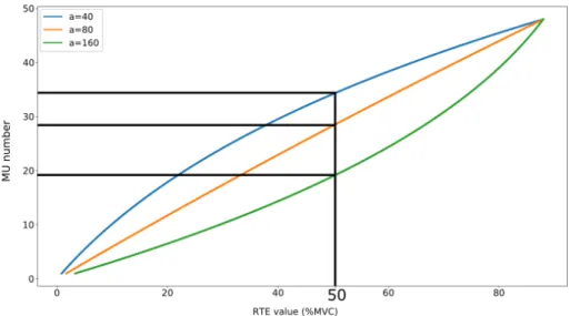
The spatial recruitment of the MUs is modulated by the intensity of contraction and follow a rule called the "size principle" defined by Henneman and al. [18, 19]. The "size principle" assessed that during isometric contraction the recruitment of MUs is done through increasing the motoneuron size and thus, the MU size. Thus, MUs are recruited from the MU innervated by the smallest diameter motoneuron to the MU innervated by the highest diameter. Each MU is excited according to the goal of the contraction level, if the goal is below its intensity threshold, the MU is not recruited for this contraction. It has been assessed that the MU recruitment law describing the evolution of the MUs threshold according to contraction level is exponential [20]. Depending on the muscle characteristics, all the MUs are recruited for a contraction level varying between 60 and 90% of the Maximal Voluntary Contraction (MVC) [21]. Beyond this threshold, only increasing the MU firing rate can increase the generated force.

In complement to the MUs spatial recruitment, the CNS also controls the MU rate coding. When a MU is recruited, the motoneuron discharges follow random point pro-cesses at a minimal frequency that increases according to the increase of the contraction level following a specific rise [20]. In the literature, we found studies defining different type of rate coding strategies [20, 22, 23, 21]. These strategies can be linear or non linear with defined minimal and maximal discharge frequencies according to the muscle char-acteristics [23, 21]. The minimal frequency varies between 3 to 10 Hz and the maximal frequency can vary from 7 to 150 Hz [2]. The MU firing regularity can be assessed by computing the Coefficient of Variation (CoV) determined on the Inter Spike Intervals (ISI), corresponding to the elapsed time between two successive firings, which is supposed

to respect a Gaussian distribution [20].

Moreover, according to [5] during natural movements, the MU recruitment pattern varies and doesn’t hold to the size principle. Size principle recruitment ensures that the slowest, most fatigue resistant MUs are recruited first for any given task. In contrary, the faster, very fatiguing MUs are therefore reserved for infrequent, high intensity tasks such as jumping. Studies on humans have shown that auditory and visual feedback can alter recruitment orders [24]. It has been suggested that MUs, within an individual muscle, may form groups that can be independently activated to fulfill specific functional roles [25]. These pools of MUs have been termed "task groups" and have showed to be selectively recruited for different kinematic conditions within a motor task such as a stride or a grasping movement [26]. It is, therefore, likely that recruitment strategies other than those predicted by the size principle may be used during gait.

Considering the specific focus upon the muscular contraction physical phenomena, we decided to use a MU recruitment pattern based on the size principle that correctly describe the MU recruitment pattern during isometric contractions [20].

1.3.2

Skeletal muscle

Macroscopic anatomy

The skeletal muscles are attached to bones by the tendons, they are in charge to produce the body motion, to maintain the posture, to produce heat and to protect the inner organs and the body. In the human body, the skeletal muscles have a variety of shapes depending on its fiber orientations and on whether the tendon junction is aligned with the tendon (fusiform muscle) or is at an angle (pennated muscle). In the case of pennated muscles, the muscle fibers are connected to the aponeurosis of the muscle [27]. Thus, we can classify the skeletal muscles according to their forms as illustrated in Fig 1.5.

Considering the complex shapes describing the skeletal muscles and thus, specific interactions acting, we had to orientate the model to only one shape description as a first modeling effort. We decided to start to describe the fusiform muscles, such as the Biceps Brachii.

The skeletal muscles of the human body are surrounded by connective tissue, which protects the muscles. The outermost of these connective tissues is called the hypodermis, located just below the skin. In addition to protecting the muscles, its role is also to regulate the heat loss generated by the muscles as well as to store the triglyceride surplus of the human body. Below this layer is a set of connective tissues, called fascia or aponeurosis (see Figure 1.6), continuously surrounding the muscle and some sub-parts.

These fascia are present in all the muscle up to the tendon to form what is defined as the myotendinous junction. The tendon then extends to the bone to form what is called the osteo-tendinous junction.

Microscopic anatomy

The most important component in the skeletal muscle is the muscle fiber which includes several hundred nuclei. The muscle fiber diameter varies from 10 µm to 100 µm according to the considered muscle. Similarly, its length differs depending on the muscle and varies between 10 and 30 cm in a healthy adult human body. Like all cells in the human body, the muscle fibers are surrounded by a plasma membrane called the sarcolemma. Com-bined with the sarcolemma, thousands of tunnel-shaped transverses tubules connect

Figure 1.5: Variety of muscle architecture in the human body.

Figure 1.6: Macroscopic structure of skeletal muscle.

the center of the muscle fiber with the outside. Inside the sarcolemma is the sarcoplasm, corresponding to the cytoplasm of the fiber. Similar to the cytoplasm, the sarcoplasm mainly holds glycogen, used for the synthesis of adenosine triphosphate (ATP) which acts

as energitical supply for the fiber [15]. In addition, myoglobin protein is also found in sar-coplasm. This protein only exists in the muscles of vertebrates. It stores oxygen molecules for the formation of ATP by the mitochondria when needed. Inside the sarcoplasm there are also numerous cylindrical subunits extending all along the muscle. These subunits are called myofibrils (muscle fibrils) (see Figure 1.7). These myofibrils are the smallest contractile units in the muscle, with a diameter of about 2µm. Around each fiber, myofib-rils are fluid-filled membrane bags called the sarcosplasmic reticulum (SR). When the muscle is at rest, the SR stores a certain amount of calcium ions (Ca2+_{). Then, during}

muscle contraction following a neural command from the CNS, the SR will release the Ca2+ _{stored in the fiber in order to realize the muscle contraction (see section 1.3.3).}

Figure 1.7: Microscopic structure of a skeletal muscle fiber.

Each myofibril consists of several small structures placed in series called sarcomeres. The sarcomere is an arrangement of several proteins defining three different filaments (see Figure 1.8):

• The thick filaments composed of myosin with a diameter of 16 nm and a length of 1-2 µm;

• The thin filament consisting of actin with a diameter of 8 nm and a length of 1-2 µm;

• The elastic filaments composed of titine.

To each thick filament is associated two thin filaments. Moreover, at the end of each thick filament is embedded an elastic filament going up to the Z disk. The Z disk is the zone that separates the sarcomeres within the myofibril. The thin and thick filaments overlap over a certain length depending on whether the muscle is relaxed, stretched or contracted. Thus each sarcomere can be decomposed into several visible bands using an electronic microscope. There is the A Band extending along the thick filament. In this band, there are two zones of superposition with the thin filaments placed at the ends. The area where there is no superposition of thin filaments is called the H band. In the middle of this H band, there is a line formed of proteins supporting the thick filaments, this support is called the M line. Finally, we define the I bands which contain the parts of the thin filaments that does not overlap and the thin filament up to the thick filament of the neighboring sarcomere (see Figure 1.7).

Figure 1.8: Anatomic structure of a muscle myofibril.

Fiber types

As stated in section 1.3.1, a MU is the set of fibers innervated by the same α-motoneuron. Thus, all of the fibers composing a MU possess the same biochemical, histochemical and contractile properties. The identification of the type of MU through its physiological properties is still a challenge today. Most studies attempt to quantify the amount of fibers according to their type by a histochemical study from a cross section of the muscle [28, 29, 30] (see Figure 1.9).

Figure 1.9: Histochemical appearance of different types of fiber in the Brachialis muscle [28].

Despite the difficulty of classification, the type of the MU is determined according to the properties of its fibers. According to published studies, fibers can be categorized into two main groups, type I fibers and type II fibers.

the fibers generating the least force. They appear dark red in the histochemical study (see Fig. 1.9) because they contain a large amount of myoglobin and blood capillaries. These fibers synthesize Adenosine TriPhosphate (ATP) mainly by the aerobic respiration of cells because they are also composed of large mitochondria. These fibers are considered to be slow because hydrolysis by the ATPase enzymes is slower than in type II fibers. Type I fibers slowly produce low force but are highly resistant to muscle fatigue and are therefore capable of providing prolonged activity and maintain it for several hours. These fibers are mainly present in the muscles responsible for maintaining the posture;

• Type II fibers (or fast fibers) have a larger diameter than type I but have less myoglobin. Therefore, they have a clearer appearance in the histochemical study (see Fig. 1.9). In addition, the release of calcium by the SR takes place more rapidly as well as the hydrolysis of the ATPase enzymes. Within fast fibers, we can also differentiate three types:

1. Type IIA fibers (or fast resistant fiber). They are similar in their composition to slow fibers and are more resistant to fatigue than other fast fibers;

2. Type IIB fibers (or fatigable fast fibers). These fibers are the closest to the definition of fast fiber, they produce a lot of force very quickly but are very sensitive to muscle fatigue;

3. The fibers of type IIC (or IIX, or intermediate fiber). These fibers are called intermediate fibers because they are in their composition and characteristics in between the fibers of type IIA and IIB.

The set of fiber types and their characteristics are summarized in Table 1.2. Table 1.1: Summary of the different types of fibers and their characteristics.

Type I Type IIA Type IIC Type IIB

Diameter Small Medium Medium Large

Myoglobin A lot A lot Moderate Little

Mitochondria A lot A lot Moderate Little

Histochemistry Dark red Red rose Light red White Contraction vilocity Slow Fast Fast Very fast

Fatigue resistance High Medium Medium Low

Generated force Low Medium Medium High

Recrutment order 1st 2nd 3rd 4th

1.3.3

Muscle contraction

Electrical phenomenon

When a neural Action Potential (AP) arrives to the NMJ, a depolarization of the fiber membrane arises. Then, an AP, called the Fiber AP (FAP), generated by this depolar-ization varies rapidly between -70 mV and 30 mV approximately as depicted in Fig.1.10 [31]. This FAP propagates along the fiber length in the two directions with a velocity that lies between 2 and 6 m.s−1 and an intensity of ∼ 100 mV.