Blink and it's done: Interactive queries on very large data

Blink and it's done: Interactive queries on very large data

The MIT Faculty has made this article openly available.

Please share

how this access benefits you. Your story matters.

Citation

Sameer Agarwal, Anand P. Iyer, Aurojit Panda, Samuel Madden,

Barzan Mozafari, and Ion Stoica. 2012. Blink and it's done:

interactive queries on very large data. Proc. VLDB Endow. 5, 12

(August 2012), 1902-1905.

As Published

http://dx.doi.org/10.14778/2367502.2367533

Publisher

Association for Computing Machinery (ACM)

Version

Author's final manuscript

Citable link

http://hdl.handle.net/1721.1/90381

Terms of Use

Creative Commons Attribution-Noncommercial-Share Alike

Blink and It’s Done: Interactive Queries on Very Large Data

Sameer Agarwal

sameerag@cs.berkeley.edu

Aurojit Panda

apanda@cs.berkeley.edu

Barzan Mozafari

barzan@csail.mit.edu

Anand P. Iyer

api@cs.berkeley.edu

Samuel Madden

madden@csail.mit.edu

Ion Stoica

istoica@cs.berkeley.edu

ABSTRACT

In this demonstration, we present BlinkDB, a massively parallel, sampling-based approximate query processing framework for run-ning interactive queries on large volumes of data. The key obser-vation in BlinkDB is that one can make reasonable decisions in the absence of perfect answers. BlinkDB extends the Hive/HDFS stack and can handle the same set of SPJA (selection, projection, join and aggregate) queries as supported by these systems. BlinkDB provides real-time answers along with statistical error guarantees, and can scale to petabytes of data and thousands of machines in a fault-tolerant manner. Our experiments using the TPC-H bench-mark and on an anonymized real-world video content distribution workload from Conviva Inc. show that BlinkDB can execute a wide range of queries up to 150× faster than Hive on MapReduce and 10 − 150× faster than Shark (Hive on Spark) over tens of terabytes of data stored across 100 machines, all with an error of 2 − 10%.

1.

INTRODUCTION

Companies increasingly derive value from analyzing large vol-umes of collected data. There are cases where analysts benefit from the ability to run short exploratory queries on this data. Examples of such exploratory queries include root-cause analysis and prob-lem diagnosis on logs (such as identifying the cause of long start-up times on a video streaming website), and queries analyzing the ef-fectiveness of an ad campaign in real time. For many such queries, timeliness is more important than perfect accuracy, queries are ad-hoc (i.e., they are not known in advance), and involve processing large volumes of data.

Achieving small, bounded response times for queries on large volumes of data remains a challenge because of limited disk band-widths, inability to fit many of these datasets in memory, network communication overhead during large data shuffles, and straggling processes. For instance, just scanning and processing a few ter-abytes of data spread across hundreds of machines may take tens of minutes. This is often accompanied by unpredictable delays due to stragglers or network congestion during large data shuffles. Such delays impact an analyst’s ability to carry out exploratory analysis on data.

In this demonstration, we introduce BlinkDB, a massively par-allel approximate-query processing framework optimized for inter-active answers on large volumes of data. BlinkDB supports SPJA-style SQL queries. Aggregation queries in BlinkDB can be an-notated with either error or maximum execution time constraints. As an example, consider a table Sessions, storing the web sessions of users browsing a media website, with five columns: SessionID, Genre, OS (running on the user’s device), City, and URL (of the website visited by the user). The following query in BlinkDB will return the frequency of sessions looking at media in the “western” Genrefor each OS to within a relative error of ±10% with 95% confidence.

SELECT COUNT(*) FROM Sessions

WHERE Genre = ’western’ GROUP BY OS

ERROR 0.1 CONFIDENCE 95%

Similarly, given the query below, BlinkDB returns an approximate count within 5 seconds along with the estimated relative error at the 95% confidence level.

SELECT COUNT(*), ERROR AT 95% CONFIDENCE FROM Sessions

WHERE Genre = ’western’ GROUP BY OS

WITHIN 5 SECONDS

BlinkDB accomplishes this by pre-computing and maintaining a carefully-chosen set of samples from the data, and executing queries on an appropriate sample to meet the error and time con-straints of a query. To handle queries over relatively infrequent sub-groups, BlinkDB maintains a set of uniform samples as well as several sets of biased samples, each stratified over a subset of columns.

Maintaining stratified samples over all subsets of columns re-quires an exponential amount of storage, and is hence impractical. On the other hand, restricting stratified samples to only those sub-sets of columns that have appeared in past queries limit applica-bility for ad-hoc queries. Therefore, we rely on an optimization framework to determine the set of columns on which to stratify, where the optimization formulation takes into account the data dis-tribution, past queries, storage constraints and several other system-related factors. Using these inputs, BlinkDB chooses a set of sam-ples which would help answer subsequent queries, while limiting additional storage used to a user configurable quantity. The sam-ples themselves are both multi-dimensional (i.e., biased over dif-ferent columns), and multi-resolution. The latter means that we maintain samples of a variety of sizes, enabling BlinkDB to effi-ciently answer queries with varying accuracy (or time) constraints,

while minimizing response time (or error). More details about the optimization problem formulation can be found in [4].

For backward compatibility, BlinkDB seamlessly integrates with the HIVE/Hadoop/HDFS [1] stack. BlinkDB can also run on Shark (Hive on Spark) [6], a framework that is backward compatible with Hive, both at the storage and language layers, and uses Spark [10] to reliably cache datasets in memory. As a result, a BlinkDB query that runs on samples stored in memory can take seconds rather than minutes. BlinkDB is open source1and several on-line service com-panies have already expressed interest in using it.

In this demo, we will show BlinkDB running on 100 Amazon EC2 nodes, providing interactive query performance over a 10 TB dataset of browser sessions from an Internet company (similar to the Sessions table above.) We will show a collection of queries focused on identifying problems in these log files. We will run BlinkDB as well as unmodified Hive and Shark and show that our system can provide bounded, approximate answers in a fraction of the time of the other systems. We will also allow attendees to issue their own queries to explore the data and BlinkDB’s performance.

2.

SYSTEM OVERVIEW

In this section, we describe the settings and assumptions in which BlinkDB is designed to operate, and provide an overview of its design and key components.

2.1

Setting and Assumptions

BlinkDB is designed to operate like a data warehouse, with one large “fact” table. This table may need to be joined with other “di-mension”tables using foreign-keys. In practice, dimension tables are significantly smaller and usually fit in the aggregate memory of the cluster. BlinkDB only creates stratified samples for the “fact” table and for the join-columns of larger dimension tables.

Furthermore, since our workload is targeted at ad-hoc queries, rather than assuming that exact queries are known a priori, we as-sume that query templates (i.e., the set of columns used in WHERE and GROUP-BY clauses) remain fairly stable over time. We make use of this assumption when choosing which samples to create. This assumption has been empirically observed in a variety of real-world production workloads [3, 5] and is also true of the query trace we use for our primary evaluation (a 2-year query trace from Con-viva Inc). We do not assume any prior knowledge of the specific values or predicates used in these clauses.

Finally, in this demonstration, we focus on a small set of ag-gregation operators: COUNT, SUM, MEAN, MEDIAN/QUANTILE. However, we support closed-form error estimates for any combina-tion of these basic aggregates as well as any algebraic funccombina-tion that is mean-like and asymptotically normal, as described in [11].

2.2

Architecture

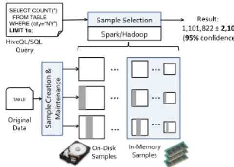
Fig. 1 shows the overall architecture of BlinkDB, which extends Hive [1] and Shark [6]. Shark is backwards compatible with Hive, and runs on Spark, a cluster computing framework that can cache inputs and intermediate data in memory. BlinkDB adds two major components: (1) a component to create and maintain samples, (2) a component for predicting the query response time and accuracy and selecting a sample that best satisfies given constraints.

2.2.1

Sample Creation and Maintenance

This component is responsible for creating and maintaining a set of uniform and stratified samples. We use uniform samples over the entire dataset to handle queries on columns with relatively uniform 1 http://blinkdb.cs.berkeley.edu Sample&Selection& TABLE& … … … … … … In)Memory& Samples& On)Disk& Samples& Original&& Data& Spark/Hadoop& & SELECT COUNT(*)! FROM TABLE! WHERE (city=“NY”)! LIMIT 1s;! HiveQL/SQL& Query& Result:) 1,101,822)±)2,105&& (95%)confidence)) Sa m pl e& Cre at io n& & & Main ten an ce&

Figure 1: BlinkDB architecture.

distributions, and stratified samples (on one or more columns) to handle queries on columns with less uniform distributions.

Samples are created, and updated based on statistics collected from the underlying data (e.g., histograms) and historical query templates. BlinkDB creates, and maintains a set of uniform sam-ples, and multiple sets of stratified samples. Sets of columns on which stratified samples should be built are decided using an opti-mization framework [4], which picks sets of column(s) that (i) are most useful for evaluating query templates in the workload, and (ii) exhibit the greatest skew, i.e., have distributions where rare values are likely to be excluded in a uniform sample. The set of samples are updated both with the arrival of new data, and when the work-load changes.

2.2.2

Run-time Sample Selection

To execute a query, we first select an optimal set of sample(s) that meet its accuracy or response time constraints. Such sample(s) are chosen using a combination of pre-computed statistics and by dynamically running the query on smaller samples to estimate the query’s selectivity and complexity. This estimate helps the query optimizer pick an execution plan as well as the “best” sample(s) to run the query on– i.e., one(s) that can satisfy the user’s error or response time constraints.

2.3

An Example

To illustrate how BlinkDB operates, consider the example, shown in Figure 2. The table consists of five columns: SessionID, Genre, OS, City, and URL.

Sess. Genre OS City URL

Query Templates

(City)

(OS, URL)

TABLE Family of random samples Family of stratified samples on {City} Family of stratified samples on {OS,URL} … … … City Genre Genre AND City URL OS AND URL 30% 25% 18% 15% 12%

Figure 2: An example showing the samples for a table with five columns, and a given query workload.

Figure 2 shows a set of query templates and their relative fre-quencies. Given these templates and a storage budget, BlinkDB creates several samples based on the query templates and statistics about the data. These samples are organized in sample families, where each family contains multiple samples of different granu-larities. In our example, BlinkDB decides to create two sample families of stratified samples: one on City, and another one on (OS, URL).

For every query, BlinkDB selects an appropriate sample family and an appropriate sample resolution to answer the query. In gen-eral, the column(s) in the WHERE/GROUP BY clause(s) of a query may not exactly match any of the existing stratified samples. To get around this problem, BlinkDB runs the query on the smallest resolutions of available sample families, and uses these results to select the appropriate sample.

3.

PERFORMANCE

This section briefly discusses BlinkDB’s performance across a variety of parameters. A more detailed comparison can be found in [4]. All our experiments are based on a 17 TB anonymized real-world video content distribution workload trace from Conviva Inc [2]. This data is partitioned across 100 EC2 large instances2 and our queries are based on a small subset of their original query trace. The entire data consists of around 5.5 billion rows in a sin-gle large fact table with 104 columns (such as, customer ID, city, media URL etc.)

1 10 100 1000 10000 100000 1e+06 2.5TB 7.5TB Qu ery R esp onse T ime (se con ds)

Input Data Size (TB) Hive on Hadoop Hive on Spark (without caching) Hive on Spark (with caching) BlinkDB (1% relative error)

Figure 3: A comparison of response times (in log scale) in-curred by Hive (on Hadoop), Shark (Hive on Spark) – both with and without full input data caching, and BlinkDB, on sim-ple aggregation.

3.1

To Sample or Not to Sample?

We compared the performance of BlinkDB versus frameworks that execute queries on the full-size datasets. In this experiment, we ran on two subsets of the raw data– of size 7.5 TB and 2.5 TB re-spectively, spread across 100 machines. Please note that these two subsets are picked in order to demonstrate some key aspects of the interaction between data-parallel frameworks and modern clusters with high-memory servers. While the smaller 2.5 TB dataset can be be completely cached in memory, datasets larger than 6 TB in size have to be (at least partially) spilled to disk. To demonstrate the significance of sampling even for the simplest analytical queries, we ran a simple query that computed average user session times with a filtering predicate on the date column (dt) and a GROUP BY on the city column. We compared the response time of the full (accurate) execution of this query on Hive [1] on Hadoop MapRe-duce, Hive on Spark (called Shark [6]) – both with and without in-put caching, against its (approximate) execution on BlinkDB with a 1% error bound for each GROUP BY key at 95% confidence and report the results in Fig. 3. Note that the Y axis is in log scale. In all cases, BlinkDB significantly outperforms its counterparts (by a factor of 10 − 150×), because it is able to read far less data to com-pute an answer. For both data sizes, BlinkDB returned the answers in a few seconds as compared to thousands of seconds for others. In the 2.5 TB run, Shark’s caching capabilities considerably help in 2_{Amazon EC2 extra large nodes have 8 CPU cores (2.66 GHz),} 68.4 GB of RAM, with an instance-attached disk of 800 GB.

0 5 10 15 20 1 20 40 60 80 100

Query Latency (seconds)

Cluster Size (# nodes) Selective + Cached Selective + No-Cache Bulk + Cache Bulk + No-Cache

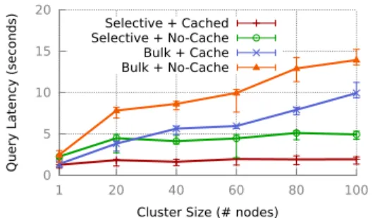
Figure 4: Query latency across 2 different query workloads (with cached and non-cached samples) as a function of cluster size

bringing the query runtime down to about 112 seconds. However, with 7.5 TB data size, a considerable portion of data is spilled to disk and the overall query is considerably affected due to outliers.

3.2

Scaling Up

In order to evaluate the scalability properties of BlinkDB as a function of cluster size, we created 2 different sets of query work-load suites consisting of 40 unique Conviva-like queries each. The first set (marked as selective) consists of highly selective queries– i.e.,those queries which only operate on a small fraction of input data. These queries occur frequently in production workloads and consist of one or more highly selective WHERE clauses. The second set (marked as bulk) consists of those queries which are intended to crunch huge amounts of data. While the former set’s input is generally striped across a small number of machines, the latter set of queries generally runs on data stored on a large number of ma-chines thereby incurring a relatively higher communication cost. Fig. 4 plots the query latency for each of these workloads suites as a function of cluster size. Each query operates on 100n GB of data (where n is the cluster size). So for a 10 node cluster, each query operates on 1 TB of data and for a 100 node cluster, each query in turn operates on around 10 TB of input data. Further, for each workload suite, we evaluate the query latency for the case when the required samples are completely cached in RAM or when they are stored entirely on disk. Since in any realistic scenario, any sam-ple may partially lie in both the disk and the memory, these results indicate the min/max latency bounds for any query.

4.

DEMONSTRATION DETAILS

BlinkDB demo will feature an end-to-end implementation of the system running on 100 Amazon EC2 machines. We will demon-strate BlinkDB’s effectiveness in successfully supporting a range of ad-hoc exploratory queries to perform root-cause analysis in a real-world scenario.

4.1

Setup Details

Our demo setup would consist of an open source implementation of BlinkDB scaling to a cluster of 100 Amazon EC2 machines. To demonstrate a real-world root-cause analysis scenario, we will pre-store approximately 10 TBs of anonymized traces of video sessions in a de-normalized fact table.

In order to effectively demonstrate the system, our demo will feature an interactive ajax-based web console as shown in Fig. 5. Users can leverage this console to rapidly query across a range of parameters and visualize any particular slice of data. In addition, we would provide a 100 node Apache Hive cluster running in par-allel for comparison.

SELECT AVG(time) FROM data

WHERE city=‘Kensington’ GROUP BY isp

WITHIN 2 SECONDS

SELECT AVG(time) FROM data

WHERE city=‘Kensington’ GROUP BY content WITHIN 2 SECONDS SELECT AVG(time) FROM data GROUP BY city WITHIN 1 SECONDS

Figure 5: A possible root-cause analysis scenario for detecting the cause of latency spikes in Kensington.

4.2

Demonstration Scenario

Our demonstration scenario places the attendees in the shoes of a Quality Assurance Engineer at CalFlix Inc., a popular (and imagi-nary) video content distribution website experiencing video quality issues. A certain fraction of their users have reported considerably long start-up times and high levels of buffering, which affect their customer retention rate and ad revenues.

Diagnosing this problem needs to be done quickly to avoid lost revenue. Unfortunately, causes might be many and varied. For example, an ISP or edge cache in a certain geographic region may be overloaded, a new software release may be buggy on a certain OS, or a particular piece of content may be corrupt. Diagnosing such problems requires slicing and dicing the data across tens of dimensions to find the particular attributes (e.g., client OS, browser, firmware, device, geo location, ISP, CDN, content etc.) that best characterize the users experiencing the problem.

As part of the demo, the attendees would be able to interactively use the web console to monitor a variety of metrics over the un-derlying data. While the top level dashboard would feature a set of aggregate statistics over the entire data, the interactive web inter-face will allow the users to compute such statistics across a specific set of dimensions and attribute values.

4.2.1

Data Characteristics

Our 10 TB workload trace would comprise of a de-normalized table of video session events. This table will consist of 100+ indi-vidual columns (e.g., session ID, session starting and ending times, content ID, OS version, ISPs, and CDNs), and it will be stored in HDFS across 100 machines. Each tuple in the table will correspond to a video session event, such as video start/stop playing, buffering, switching the bitrate, showing an ad, etc. The table will contain billions of such tuples.

4.2.2

Root-cause Analysis Scenarios

In order to demonstrate a few root-cause analysis scenarios, we would inject a number of synthetic faults in this event stream as described below:

1. Latency Spikes: In this scenario, ISP ‘XYZ’’s users in ‘Kensington, CA’experience a latency spike while watching ‘Star Wars Episode I: The Phantom Menace’ due to high contention on the edge cache.

2. Buggy Video Player: In this scenario, ‘Firefox 11.0’ users experience high-buffering times due to a buggy beta release of ‘ZPlayer’, an open-source video player.

3. Corrupted Content: In this scenario, a particular copy of a content in a CDN’s server is corrupted affecting a number of users accessing that content.

Diagnosing all these faults would involve ad-hoc analysis by in-teractivelygrouping or filtering the event table across a number of dimensions (such as ISPs, City, Content IDs, Browser IDs etc). We expect that the users would be able to detect the root-cause in all of these scenarios in a matter of minutes, hence demonstrating the effectiveness of BlinkDB in supporting interactive query analysis over very large data.

5.

RELATED WORK

Approximate Query Processing (AQP) for decision support in relational databases has been studied extensively. Such work has either focused on sampling based approaches on which we build, or on the use of other data structures; both are described below.

There is a rich history of research into the use of both random and stratified sampling for providing approximate query responses in databases. A recent example, is SciBORQ [8, 9], a data-analytics framework for scientific workloads. SciBORQ uses special struc-tures, called impressions, which are biased samples with tuples se-lected based on their distance from past query results. In contrast to BlinkDB, SciBORQ does not support error constraints, and does not provides guarantees on the error margins for results.

There has also been a great deal of work on “synopses” for answering specific types of queries (e.g., wavelets, histograms, sketches, etc.)3. Similarly materialized views and data cubes can be constructed to answer specific queries types efficiently. While offering fast responses, these techniques require specialized struc-tures to be built for every operator, or in some cases for every type of query and are hence impractical when processing arbitrary queries. Furthermore, these techniques are orthogonal to our work, and BlinkDB could be modified to use any of these techniques for better accuracy with certain types of queries, while resorting to samples for others.

Acknowledgements

This research is supported in part by gifts from Qualcomm, Google, SAP, Amazon Web Services, Blue Goji, Cloudera, Ericsson, Gen-eral Electric, Hewlett Packard, Huawei, IBM, Intel, MarkLogic, Microsoft, NEC Labs, NetApp, Oracle, Quanta, Splunk, VMware and by DARPA (contract #FA8650-11-C-7136).

6.

REFERENCES

[1] Apache Hive Project. http://hive.apache.org/. [2] Conviva Inc. http://www.conviva.com/.

[3] S. Agarwal, S. Kandula, N. Bruno, M.-C. Wu, I. Stoica, and J. Zhou. Re-optimizing Data Parallel Computing. In NSDI, 2012.

[4] S. Agarwal, A. Panda, B. Mozafari, S. Madden, and I. Stoica. BlinkDB: Queries with Bounded Errors and Bounded Response Times on Very Large Data. Technical Report, http://arxiv.org/abs/1203.5485, 2012.

[5] N. Bruno, S. Agarwal, S. Kandula, B. Shi, M.-C. Wu, and J. Zhou. Recurring Job Optimization in Scope. In SIGMOD, 2012.

[6] C. Engle, A. Lupher, R. Xin, M. Zaharia, M. Franklin, S. Shenker, and I. Stoica. Shark: Fast Data Analysis Using Coarse-grained Distributed Memory. In SIGMOD, 2012.

[7] M. Garofalakis and P. Gibbons. Approximate Query Processing: Taming the Terabytes. In VLDB, 2001. Tutorial.

[8] M. L. Kersten, S. Idreos, S. Manegold, and E. Liarou. The Researcher’s Guide to the Data Deluge: Querying a Scientific Database in Just a Few Seconds. PVLDB, 4(12), 2011.

[9] L. Sidirourgos, M. L. Kersten, and P. A. Boncz. SciBORQ: Scientific data management with Bounds On Runtime and Quality. In CIDR’11, pages 296–301, 2011.

[10] M. Zaharia et al. Resilient Distributed Datasets: A Fault-Tolerant Abstraction for In-Memory Cluster Computing. In NSDI, 2012.

[11] K. Zeng, B. Mozafari, S. Gao, and C. Zaniolo. Uncertainty Propagation in Complex Query Networks on Data Streams. Technical report, UCLA, 2011. 3