Autonomous cooperation of heterogeneous platforms for sea-based search tasks

(1)

Autonomous Cooperation of Heterogeneous

Platforms for Sea-based Search Tasks

by

Andrew J. Shafer

Submitted to the Department of Electrical Engineering and Computer

Science

in partial fulfillment of the requirements for the degree of

Master of Engineering in Electrical Engineering and Computer Science

at the

MASSACHUSETTS INSTITUTE OF TECHNOLOGY

June 2008

c

Massachusetts Institute of Technology 2008. All rights reserved.

Author . . . .

Department of Electrical Engineering and Computer Science

May 23, 2008

Certified by . . . .

John J. Leonard

Professor

Thesis Co-Supervisor

Certified by . . . .

Michael R. Benjamin

Visiting Scientist

Thesis Co-Supervisor

Accepted by . . . .

Arthur C. Smith

Chairman, Department Committee on Graduate Theses

(2)

(3)

Autonomous Cooperation of Heterogeneous Platforms for

Sea-based Search Tasks

by

Andrew J. Shafer

Submitted to the Department of Electrical Engineering and Computer Science on May 23, 2008, in partial fulfillment of the

requirements for the degree of

Master of Engineering in Electrical Engineering and Computer Science

Abstract

Many current methods of search using autonomous marine vehicles do not adapt to changes in mission objectives or the environment. A cellular-decomposition-based framework for cooperative, adaptive search is proposed that allows multiple search platforms to adapt to changes in both mission objectives and environmental param-eters. Software modules for the autonomy framework MOOS-IvP are described that implement this framework. Simulated and experimental results show that it is feasi-ble to combine both pre-planned and adaptive behaviors to effectively search a target area.

Thesis Co-Supervisor: John J. Leonard Title: Professor

Thesis Co-Supervisor: Michael R. Benjamin Title: Visiting Scientist

(4)

(5)

Acknowledgments

I would like to thank Professor John Leonard and Dr. Michael Benjamin for taking me on as a UROP student and guiding my research. I also want to thank Professor Henrik Schmidt for providing financial support for my M.Eng.

The Office of Naval Research supported my participation in a research cruise to Dabob Bay, WA where I learned more about marine vehicle operations. I am also indebted to the researchers at NSWC–Panama City, FL for teaching me the basics of mine warfare and mine countermeasures. Special thanks go to Rafael Rodriguez for his “MCM 101” presentation and Gerald Dobeck for his talk about CAD/CAC.

Joe Curcio taught me many things about the kayaks and real-world engineering trade-offs. Kevin Cockrell was invaluable as a person to bounce ideas off. Toby Schneider knew all of the little tricks for conducting successful water operations.

Finally, I want to thank all of my family and friends for their support throughout the years. Without them I never would have thought it possible to graduate.

(6)

(7)

List of Figures

1-1 Operator-led search for mine-like objects . . . 18

1-2 SeeByte’s onboard CAD/CAC module . . . 18

1-3 Bluefin’s 21-inch AUV . . . 20

1-4 The SCOUT autonomous kayak . . . 21

1-5 The MOOS architecture . . . 22

1-6 The IvP Helm, pHelmIvP . . . 23

1-7 An objective function for a waypoint behavior . . . 23

2-1 Planning goal for mine countermeasures . . . 27

2-2 Lateral range curve . . . 28

2-3 A-B sensor model . . . 29

2-4 Corrections to P for MCM operations . . . 29

2-5 Squence showing the updated clearance of a cell. . . 31

3-1 Data flow diagram for the toolchain . . . 36

3-2 Search areas and search grids . . . 38

3-3 Communication paths for grid updates . . . 39

3-4 Multiple objective function setup . . . 42

3-5 Multiple objective functions in pIvPHelm . . . 43

4-1 Kayak searching behind an AUV . . . 52

4-2 Kayak searching behind an AUV without slew-rate limiting . . . 53

4-3 Effects of the environment on lawnmower behaviors . . . 56

(12)

4-5 Different sensor module mission. . . 64

4-6 Different sensor module mission–fast lead . . . 66

C-1 . . . 83

C-2 . . . 84

C-3 . . . 85

(13)

List of Tables

2.1 Basic signal-detection theory terminology . . . 32

4.1 Scoring metrics used in simulation/experimental evaluation . . . 48

4.2 Summary of simulations and experiments . . . 49

4.3 Sim./exp. results for mission 4.1 . . . 52

4.7 Sim./exp. results for mission 4.5.1 . . . 64

(14)

(15)

Chapter 1 Introduction to Autonomous Mine

Countermeasures

1.1 Project Goals

The goal of this project is to design and implement a software system to enable multiple marine vehicles to search a given area. Specifically, tools are needed to 1) model sensor performance, 2) maintain and synchronize a map of the area, and 3) implement a search algorithm.

1.2 Limitations of Current Search Methods

Previous research in the searching domain has focused on “lawnmower” style patterns of mapping an area [4, 15, 26, 42–44]. However, this process deteriorates as more vehicles are added. If a vehicle is assigned to a portion of the overall area and then breaks down, the other vehicles must be manually reconfigured to scan that portion. Also, this process generally assumes the platforms are identical and does not take advantage of the capabilities that may be unique to each vehicle (e.g. one may have side-scan sonar, one forward-looking sonar, another optical or magnetic sensors, etc.). Finally, this process does not allow for cooperation with other objectives of the vehicle, such as collision avoidance or periodic surfacing.

(16)

Current search algorithms also generally assume a constant probability of detec-tion for the targets they seek. This assumpdetec-tion may not be realistic for real-world environments where the motion of the water and the composition of the sea-bottom can vary drastically.

Previous research in AUV behavior development has primarily focused on imple-menting behaviors for a single vehicle [10–12], such as a single AUV taking tempera-ture readings during ocean trials. With access to larger numbers of autonomous craft, research is now needed to explore possible ways for these vehicles to interact [6, 34], especially if the vehicles have different capabilities (such as an autonomous surface vehicle and an autonomous underwater vehicle, see [47]).

1.3 Background

1.3.1 A Brief Overview of Mine Countermeasures (MCM)

The ultimate goal of mine countermeasures (MCM) is to neutralize mines (called targets). There are two basic ways to go about this, minesweeping and mine hunt-ing. Minesweeping refers to the process of neutralizing all mines in an area without specifically locating them first. This might involve, for example, using a helicopter to tow a large ferrous sled through mined waters, hoping to activate the mines so that they no longer pose a threat to area shipping traffic. Mine hunting, on the other hand, involves locating, detecting, and classifying mines for later neutralization. This neutralization might be done by the mine hunting vehicle itself, or it might be done by Navy divers or specialized vehicles. (For a more thorough introduction, see [25].) Minesweeping is typically done after the conflict is over. Its objective is to clear an entire area to allow commercial and military shipping to safely move through the area. Mine hunting, however, might be done in hostile waters, such as clearing the waters near an enemy beach for an amphibious assault. This means that minehunters (either vessels or divers) often need to be discrete and difficult to detect.

(17)

mines, marking their locations, and setting explosive charges for later detonation. This process is very accurate with regards to the detected targets but is extremely time consuming, expensive, and also dangerous for covering large areas.

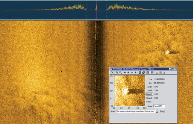
This process was improved with the invention of sonar which allowed single ships to map the seafloor. This sonar data was then processed into a graphical form that a trained operator would look at to mark the mine-like objects (see Figure 1-1). At this point it is beneficial to explain the terminology for mine hunting. Mine hunting involves two steps; the first step is detection. For the detection phase, an oil drum, a large rock, and a mine should all be “detected”. The second step is classification. Classification is determining which objects are mine-like and which are not. For this example, the oil drum and mine could both be considered mine-like. These two phases are defined as mine-hunting. (To complete the description of mine countermeasures: the third phase, identification, seperates mines (the targets) from non-mines (the clutter). The first three phases are sometimes referred to as DCI. The fourth phase, neutralization, eliminates the threat from the mines.) [36]

The maturing of autonomous underwater vehicles (AUVs, or unmanned undersea vehicles, UUVs) initially automated the data-collection phase of mine hunting. That is, AUVs were programmed to follow a lawnmower style path over a search region, record data, and then return home. The AUVs were retreived and the data was downloaded to a computer where trained operators would look at the images to detect and classify mine-like objects. This automated data collection allowed a large search area to be covered efficiently, but still required operators to look over hundreds of images to identify mine-like objects. This procedure is tiring and demanding on the human operators.

The next advancement in mine hunting detection and classification was using com-puter image processing to pre-screen the images, assisting the operator by pointing out obvious targets. The automated detection and classification of mine-like objects is called CAD/CAC (computer-aided detection/computer-aided classification). Recent advances in image processing, combined with space and energy efficient computers (see Figure 1-2), have now allowed CAD/CAC to be performed onboard the AUV.

(18)

Figure 1-1: MCM operators look for proud mine-like objects in side-scan sonar images. Detection and classification can be easy in simple terrains like this but increases in difficulty as the amount of clutter (such as rocks and other large debris) increase. Image courtesy Bluefin Robotics.

Figure 1-2: This small, power-efficient CAD/CAC module by SeeByte allows for the onboard detection and classification of mine-like objects on an AUV.

(19)

Currently, the only advantage that onboard CAD/CAC provides is that the AUV can communicate a “top-ten” list of targets while still searching, allowing vessels to begin identification and neutralization before the entire area has been scanned. The AUVs, however, do not use the information they have gained to alter their search patterns. A active area of research in this field is to try to close the loop and allow the AUV to autonomously make adjusts to its plan based on the information it is gathering.

1.3.2 Autonomous Underwater/Surface Vehicles (AUVs/ASV)

Autonomous underwater vehicles come in a variety of sizes, from 9-inch diameter man-portable units like Hydroid’s REMUS1 _{all the way up to Bluefin’s 21-inch diameter}

BPAUV2 _{(see Figure 1-3). The larger units are equipped with acoustic modems, more}

sophisticated sensors, larger batteries, and the capability of towing acoustic sensors. The smaller units are generally more energy efficient, but they often lack acoustic modems for underwater communication. All kinds of AUVs are capable of carrying some form of sonar for bottom sensing, including mine-like object detection.

Autonomous surface vehicles are now cheap and simple enough to operate that it is possible for a research group to have three to twelve of these vehicles for testing. The SCOUT platform (see Figure 1-4) of robotic kayaks cost around $30,000/unit, are equipped with GPS, a compass, a thruster capable of nearly four knots, and an off-the-shelf PC for autonomy. [18] Variants of the SCOUT have been fitted with such equipment as long-wave radios [34], acoustic modems [19] for communicating with underwater vehicles, and CTDs for taking water sound-velocity measurements. This inexpensive platform has allowed for the testing of some novel multi-vehicle experiments in collision avoidance. [10, 12]

1

http://www.hydroidinc.com/pdfs/remus100web.pdf 2

(20)

Figure 1-3: Bluefin’s 21-inch diameter AUV is capable of diving exceptionally deep for long periods of time to take readings near the ocean floor. Advanced autonomy soft-ware (see Section 1.3.3) makes the independent operation of these vehicles possible. Image courtesy Matt Grund.

(21)

Figure 1-4: The SCOUT platform of autonomous kayaks are a relatively inexpensive robotic platform. The low cost and ease-of-use make it possible for research groups to own and operate several of these vehicles. Image courtesy Mike Benjamin.

1.3.3 Autonomy Software

The autonomy software for this project is a suite of software referred to as “MOOS,” the Mission Oriented Operating Suite (by Paul Newman [31]), coupled with an interval-programming-based multi-objective optimization helm called pIvPHelm by Mike Benjamin [9]. The collective suite is referred to as MOOS-IvP.

MOOS is a platform-independent software suite that facilitates communication between processes that are typically written by different users. Each process gets information by talking only with the central MOOS database, MOOSDB (see Fig-ure 1-5). The independence of each process from every other process prevents prob-lems with one process from taking down the whole system. To share information, processes publish data to the MOOSDB in a (Name, Value) pair. Other processes that are interested in this data subscribe to the (Name) variable and are informed of updates to this variable by the MOOSDB. The modularity of this system en-forces firm, clear interfaces between processes that desire to communicate with one another. For instance, the GPS software might publish variables called GPS LAT and

(22)

in-Logger 2Hz 20Hz 5Hz 40Hz 4Hz 8Hz 5Hz 10Hz MicroModem Tracker pNav ThrustControl GPS MOOSBridge IvP Helm

MOOSDB

Figure 1-5: The Mission Oriented Operating Suite (MOOS) by Paul Newman is a middle-ware software suite that facilitates communication between different processes in a publish-subscribe architecture. Image courtesy Mike Benjamin.

ternal compass might publish COMPASS HEADING. The navigation software (e.g., pNav) would subscribe to these variables and publish NAV Xand NAV Y, its best estimate as

to the location of the vehicle. Other software could subscribe to this navigation data and publish a desired heading and speed, while rudder and thruster control software could subscribe to the desired heading and speed data and actually interface with those physical controls.

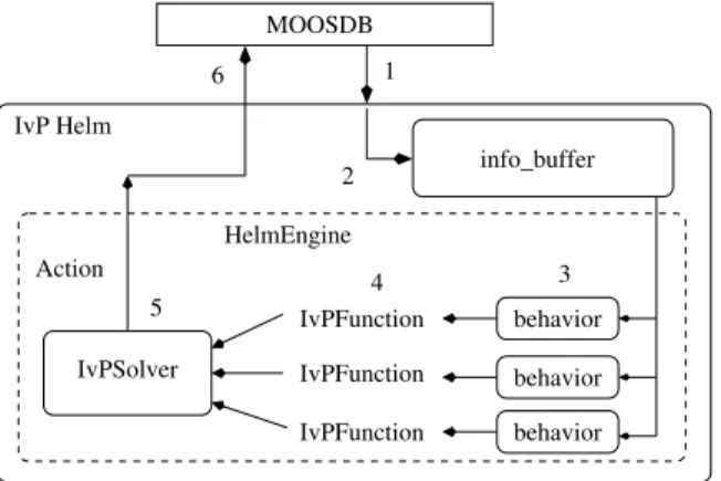
MOOS, as robot middleware, does not provide much in the way of vehicle au-tonomy. The MOOS software distribution does provide a simple helm process called pHelm. Multi-objective optimization between behaviors is implemented in another MOOS process called pHelmIvP a.k.a. the IvP Helm. [8] In the MOOS publish-subscribe architecture, pHelmIvP publish-subscribes to variables such asNAV X, NAV Y, NAV HEADING,NAV SPEED, and others (such as the position, heading, and speed of other vehicles) and typically publishesDESIRED HEADING and DESIRED SPEED.

pHelmIvP produces the desired heading and speed for a vehicle by efficiently weighing and optimizing the combination of objective functions produced by individ-ual behaviors (see Figure 1-6). As a simple example, suppose a waypoint behavior produces an objective function that desires a course that would take the vehicle to a desired waypoint at a specified speed (see Figure 1-7). Also suppose there is a behav-ior that desires to limit the rate of turn of a vehicle to prevent kinking a tow cable. In some architectures, the helm would choose one behavior over another to control

(23)

the vehicle. In our example this would either cause the vehicle never to reach the waypoint, or the vehicle to turn so sharp it kinks the cable. Other architectures would simply combine the single-decision output of each behavior. In our example this could violate the turn limit. pHelmIvP solves this multi-objective optimization problem by efficiently searching over the entire decision space (all discrete headings and speeds) and choosing the heading and speed that maximizes the combined objective funtions.

IvPSolver behavior behavior behavior MOOSDB 5 4 IvPFunction IvPFunction IvPFunction 3 HelmEngine Action 6 1 2 info_buffer IvP Helm

Figure 1-6: pHelmIvP uses the interval programming method to solve the competing objectives of different behaviors. Image courtesy Mike Benjamin.

90

180 270

135 0

Figure 1-7: In this visualization of an objective for a waypoint behavior, the behavior would like to procede to a point at heading 135 degrees, but it is willing to take courses that take it near the point too. Image courtesy Mike Benjamin.

1.3.4 A Note on Coverage

In many applications of multiple vehicle problems, the goal is to “cover” an area with some kind of sensor. This includes such applications as mine deployment and mine hunting, robotic automobile painting [15], automated cleaning robots [30], and others. It is important to distinguish the different types of coverage that can be achieved. [20]

(24)

There are three basic types of coverage:

1. Blanket or Field Coverage is a static way of arranging your search elements such that you minimize the probability of a target appearing undetected inside the search area.

2. Barrier Coverage is a static arrangement of search elements that attempts to minimize the probability that a target passes undetected through the barrier. 3. Sweep Coverage is a dynamic arrangement of search elements that moves

through the search area, attempting to both maximize the number of detections per time and to minimize the number of missed detections.

It is also important to recognize the capabilities of the targets when designing a coverage program. For static targets, any patterns that cover the entire area are essentially equivalent detection-wise. Moving targets, however, could conceivably do something like follow behind the searcher, preventing their detection even if the entire area is “covered” by the moving search elements. For adversarial moving targets like these, some form of moving barrier coverage is desired.

1.3.5 Relevance of Cooperative, Autonomous, Adaptive Search

The applications of this research are valuable for both military and civilian purposes. The Navy is currently funding research initiatives for cooperative search platforms that can search large (100-km by 100-km) areas. [32] There are also combined Navy and civilian efforts, such as PLUSNet, that are attempting to expand the communi-cation capabilities of underwater vehicles. [24, 40]

1.4 A Novel Approach to Adaptive Autonomous

Search

(25)

1. Mine hunting is the only task the vehicle is trying to complete, allowing the search algorithm to completely determine the actions of the vehicle.

2. The sensor’s detection ability is constant for all regions of the search area and does not depend on environmental conditions or vehicle state (these parameters are referred to as the sensor’s A and B values, see Section 2.1).

These two assumptions preclude using an adaptive algorithm for mine hunting. By violating these assumptions I propose a novel solution of decomposing the search area into smaller cells that allows for adaptive autonomous mine hunting. In particular, the algorithm is adaptive to changes in:

1. The mission, by allowing multiple objectives to be completed simultaneously, and

2. The environment, by adjusting the sensor’s A and B parameters.

1.5 Criteria for Success

Defining success for search tasks is not easy and various papers use different definitions of success. [39] The elements that comprise an “efficient” search algorithm greatly depend on the objectives of the searcher. For example, efficiency might be defined based on the time of search, the search platform’s cost or effectiveness, the number of missed and/or detected targets, or some other objective, such as finding a cleared path between two points.

That being said, success for this project will be defined as:

1. Creating a set of tools that enable a user to plan, simulate, and conduct a search operation over a specified area.

2. Conducting a series of simulations and experiments to show that these tools allow users to evaluation the effectiveness of their own search efforts.

(26)

1.6 Chapter Summary

In this chapter we have described the problem that current search algorithms face as being non-adaptive to real-world parameters such as the environment or mission objectives. We have also described mine countermeasures (MCM) in terms of detec-tion, classificadetec-tion, identificadetec-tion, and neutralization phases. Several real autonomous vehicles and their capabilities were examined and some of the autonomy software that runs on them was described. The thesis of this work is that because current search algorithms assume that mine hunting is the only vehicle task and that the sensor parameters are constant, those algorithms are unable to adapt to changing environ-mental and mission parameters. To remove those assumptions, we use a cellular-decomposition method to create a framework that allows environmental and mission adaptation.

The next section describes mine countermeasure theory and how it applies to the cellular decomposition.

(27)

Chapter 2 Theory

2.1 Mine Countermeasure Theory

Planning for mine countermeasures (MCM) operations takes on a probability-based framework that trades the risk of missing targets for the time spent to cover the search area. [21, 36] The current objective of this planning operation is to determine the number of search tracks, N , across the search area of channel width C to attain the desired clearance level P (average probability of neutralizing mines) (see Figure 2-1).

Figure 2-1: When planning for a mine countermeasures operation, the mission com-mander specifies a desired clearance level P , for the search area. The result of the planning is N , the number of search tracks to cover the entire channel width, C. Image courtesy Rafael Rodriguez.

(28)

de-pends on the relative locations of the searcher and target, the physical capabilities of the sensor, the physical characteristics of the target, and the environment. Because the probability of detection is very low for long distances between the searcher and target, it is possible to calculate the probability of detection for a target at a given lateral range (distance between a target the straight line trajectory of a searcher) by integrating the instantaneous probability of detection from −∞ to ∞. See Figure 2-2.

X P(X) 1.0 Imperfect Sensor X P(X)

Lateral Range Curve 1.0 Sensor Track Y Lateral Range X Target

a.

c.

X P(X) 1.0

Definite Range Law

b.

d.

Figure 2-2: In a., the sensor passes along a target at lateral range X. Integrat-ing the instantaneous detection probability (a function of X and sensor and target characteristics), we obtain a fictional b., the lateral range curve. This curve goes to 0 for large X and may not be symmetric, depending on the sensor configuration. Approximations for b. include c., which assumes that all targets within a fixed dis-tance are detected (cookie cutter), and d., which more accurately models the sensor’s performance (imperfect sensor). Image originally appears in [21].

For our purposes then, a sensor can be completely described by its nominal de-tection probability, B, and its nominal range (width), A. See Figure 2-3.

The mission commander for an MCM operation specifies a desired clearance level, P , which gives the probability that any particular mine has not been neutralized. For

(29)

X 1.0

P(X)

B

A

Figure 2-3: This model completely describes the sensor using its detection probabil-ity, B, and its range, A.

example, if the mission commander desires 96% clearance, that allows a 4% chance each mine has not been neutralized. In a field of 100 mines, it would be acceptable for four of them not to be neutralized.

With a perfect sensor (B = 1), the clearance level is just equal to the portion of the search area covered by the sensor (see Equation 2.1). For an imperfect sensor, the probability of missing any particular mine is inversely proportional to the number of times the entire area has been scanned.

P =    max(N ∗ A/C, 1) B = 1 1 − (1 − B)N ∗A/C B < 1 (2.1)

Further complicating clearance operations is that the probability of identification Pid < 1, the probability of neutralization Pn < 1, and there are some mines that

cannot be detected, µ. (See Figure 2-4) If the commander desires an overall clearance

D&C ID Neut. Detectable P

P’

Figure 2-4: Modifications need to be made to P to account for limits in Pid, Pn, and

µ. That is to say, if the commander desires 90% clearance and the product of Pid,

Pn, and 1 − µ is 97%, we can set the desired clearance level of our algorithm, P0 to

(30)

level of P , we can correct for these factors by increasing the coverage to

P0 = P/(Pid∗ Pn∗ (1 − µ)) (2.2)

Because we can correct for these factors by increasing P , we will ignore any compli-cations caused by these factors. In the case where P > (Pid∗ Pn∗ (1 − µ)), no number

of paths can satisfy the desired clearance level and a later minesweeping effort will have to be conducted.

2.2 Applications to Small Cells

The previous discussion applies to a large search area where it makes sense to talk about the number of paths that cover the search area. It is possible to apply this reasoning to small cells, which is at the heart of what we are trying to do.

Recall that the clearance level, P , is an average of 1−(the probability that an undetected target is present). Also recall that B is the probability that the sensor will detect a given target as it passes by the target. Importantly, it is assumed that detection events are independent for each target and for each pass of the sensor over the target. However, this assumption might not hold for some targets or environ-ments. For example, some targets have a strong directionality which makes them easily detectable from one direction but not from another. Applying this to a small cell, every time a cell comes into view and then leaves, we must update the clearance level of that cell. Assuming detection independence, the equation for updating a cell that has been sensed is in Equation 2.3.

new prob. missed = (prob. prev. missed) ∗ (prob. missed this time) 1 − Pnew = (1 − Pold)(1 − B)

Pnew = 1 − (1 − Pold)(1 − B) (2.3)

(31)

over a cell multiple times.

(a) (b) (c)

(d) (e) (f)

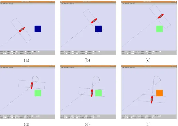
Figure 2-5: In this figure, a sensor is passed over a single cell. As the sensor enters the cell (b), nothing is changed. When the sensor has completely passed the center of the cell (c), its clearance is updated according to Equation 2.3. Here, the cell has changed from 0 clearance (blue), to .5 clearance (teal). On the second pass, (d)-(f), the cell is updated from .5 to .75 (orange); which is two passes of a .5 sensor. These updates are communicated to other searchers to adjust their own internal grids.

The average clearance for a group of cells is the average of each cell’s clearance weighted by its relative area. For equal-sized cells, this is equivalent to summing the clearances and dividing by the number of cells.

Average Clearance P =

PN i=1Pi

N

2.3 Signal Detection Scoring Metrics

The scoring metric used to evaluate a potential search algorithm greatly influences the design of that algorithm. For instance, with a metric that greatly punishes missing targets and only lightly penalizes incorrectly declaring a target, the algorithm may

(32)

decide to declare many of the objects it sees as targets. In addition to the standard signal detection theory scoring (see Table 2.3), the score might be affected by factors such as the time of search (penalizing long search times), the clearance level, the number of search vessels used, amount of energy expended, or the completion of certain objectives, such as finding a lane [33] from one side of the area to the other.

While not explored in this research, it would be beneficial to try to create a scoring metric that uses classic signal detection theory but that also incorporates each cell’s clearance level, P , when assigning points. For example, if a cell has a high clearance level, meaning that not many targets should be missed there, the penalty for misses would be increased.

Table 2.1: Basic signal detection theory terminology. Here, there are two states for each cell, either there are targets present or there are no targets present. There are also two possible outputs of the search effort, declaring a target present or not present.

Target Present Target Not-Present Declare Target Hit False Positive Declare No Target Miss Correct Rejection

To simplify the calculation of scores, we will use classic signal detection scoring. We will hold the other possible scoring variables (such as time or clearance level) constant to compare search algorithms. The actual scoring tool/metric is discussed in Appendix B.3.

2.4 Chapter Summary

In this chapter we have given an overview of the current state of mine countermeasure theory, including the current goal of operations planning of calculating N , the number of paths to use when covering a channel of width C. The clearance level, P , is a measure of how likely it is that a target has not been neutralized. This clearance level can be calculated for an entire search area (which is currently done), or it can be applied to a cellular decomposition of the search area (this research). Finally, the

(33)

scoring metric used to evaluate a search algorithm greatly influences the design of that algorithm. For this research, we use classic signal detection theory while holding other variables (such as time or clearance level) constant.

In the next chapter we describe the software modules that implement this cellular decomposition framework and the search algorithms.

(34)

(35)

Chapter 3 Software Framework and Modules

The principle development work for this project is the creation of three software modules: pSensorSim, pArtifactMapper, and bhv SearchArtifact. These software modules form a chain that starts with simulated targets and ends with desired heading and speed commands for the vehicle. pSensorSim loads the artifacts to simulate and publishes the artifacts that it detects. pArtifactMapper subscribes to these artifact updates and forms a clearance map of the area of interest. The search behavior then subscribes to this clearance map and makes decisions about where the vehicle should go next. See Figure 3-1 for a diagram of the relationship. Any of the modules can be replaced with components that follow the same interface. For example, the sensor model could be replaced with the actual sensor hardware, and the search behavior could be replaced with any other search algorithm. Configuration information for all of the software is in Appendix B.

3.1 pSensorSim

pSensorSim is a MOOS process that simulates the output of a fictional sensor given a “threat laydown,” which is a list of targets to simulate.

The algorithm for sensing is shown in Algorithm 1. The basic process is to main-tain a list of artifacts that can currently be “seen” by the sensor and store it. On the next iteration, for each new artifact, pick a random number [0, 1). If the random

(36)

pArtifactMapper

bhv_SearchArtifact pSensorSim

artificial data mock sensor output

sensor data

map of artifact field

heading, speed objective function

Figure 3-1: This diagram displays the flow of data between the three parts of the search toolchain. pSensorSim models a simple sensor and outputs the artifacts that it detects. pArtifactMapper remembers this output and also keeps track of which cells the vehicle has covered. This artifact map is used by the search behavior (bhv SearchArtifact) to produce an objective function for the helm to solve.

number is less than B (the sensor detection capability), emit the artifact as a detected artifact for processing by other modules. Now store the list of all seen artifacts for the next iteration.

Another essential function of pSensorSim is to simulate variations in the sensor’s A and B values. Recall that A is the effective width of the sensor while B is the probability that the sensor will detect any given target. pSensorSim uses a simple two-value sensor B parameter that changes the sensor’s normal value to a reduced value for a short period of time. For example, the sensor might have a B value of .8 for 60 seconds and then drop to .25 for 10 seconds before repeating the cycle. There is plenty of room for further work in modeling a sensor’s B value given the state of the vehicle and the bottom environment. See Chapter 5.2.

3.2 pArtifactMapper

pArtifactMapper’s role is to maintain two data structures: 1) a list of all the detected artifacts, and 2) a clearance level associated with each cell of the search grid.

(37)

input : threat laydown output: detected artifacts load(threat laydown);

locArtifacts ← Detect(currx, curry, currhdg); while true do

newArtifacts ← Detect(currx, curry, currhdg);

foreach artifact in newArtifacts and not in locArtifacts do x ← Rand([0, 1)); if x < B then Publish(artifact); end end locArtifacts ← newArtifacts;

/* Publish the sensor values so pArtifactMapper can adjust its

internal values */

Publish(Sensor A); Publish(Sensor B); end

Algorithm 1: Algorithm for pSensorSim. See Section 3.1 for a full description. First, some terminology. The search area is the physical region of interest, defined by a convex polygon. The convex polygon requirement is not a function of anything that pArtifactMapper can perform, but rather because the search behavior, which shares the map, currently only functions with convex polygons. This requirement could be relaxed with a reworked behavior.

3.2.1 Discretization Method

The search area polygon is completely tiled with equal-sized, square elements, forming a search grid. The total area of the search grid fully includes the area of the search area. See Figure 3-2. The size of the cells is specified by the user. For most of this work we have been using 5-m squares. This number seems to be small enough that it is within the error bounds of a sensor (approximately 8-m [41]), but large enough that the number of cells is manageble.

Other constraints might limit the maximum number of cells that can be described. For instance, if an AUV allocates 10-bits to describe the cell index number, the number of cells is limited to 1024 (210), regardless of an optimal size for the cell.

(38)

(a) A search area defined by a convex polygon. (b) The search grid that completely covers the search area.

Figure 3-2: The search area, defined by a convex polygon (a), can be broken into discrete, equal-sized, square elements that completely cover the area (b)

Also, square cells might not be the best shape for the elements. Some discretiza-tion methods use hexagonal cells because of their close-packing ability and because it removes ambiguity as to which cells are considered neighbors. [42]

3.2.2 Grid Updates

When pArtifactMapper receives a detected artifact notice from pSensorSim, it stores the artifact in the cell location that corresponds to the artifact’s X and Y values.

Using the theory developed in Section 2.2, for all cells that have entered the sensor’s effective area and then left (i.e., those cells have been scanned), those cells have their clearances updated.

Pnew = 1 − (1 − Pold)(1 − B)

Pnew = Pold+ B(1 − Pold)

(39)

as a grid update. Grid updates take the form of index, prev clearance, new clearance. The previous clearance is included in the update in case platforms want to try to reconstruct a sequence of grid updates. To communicate these updates to other vehi-cles, other MOOS processes deliver the message in whatever form is appropriate. For communication over TCP/IP channels, pMOOSBridge forms a connection to both MOOSDBs and pushes updates in one direction. Underwater, acoustic modems are used to communicate data at slow rates. Figure 3-3 shows how one community might be passing these updates.

pHelmIvP MOOSDB Kayak 2 pSensorSim pArtifactMapper MOOSDB Kayak 1 pSensorSim pHelmIvP pArtifactMapper pMOOSBridge3 pArtifactMapper pSensorSim pMOOSBridge1 pMOOSBridge2 MOOSDB AUV 1 pHelmIvP pAComms pAComms GRID_UPDATE_LOCAL GRID_UPDATE_LOCAL GRID_UPDATE_LOCAL Wi−Fi Links GRID_UPDATE GRID_UPDATE GRID_UPDATE Acoustic Modem

Figure 3-3: This diagram displays one possible way for grid updates (and other MOOS variables) to be communicated between vehicles. For the two surface vehicles with Wi-Fi connections, pMOOSBridge maintains a TCP/IP connection to both databases and is able to publish updates from one MOOSDB to another. In this example, one of the kayaks is outfitted with an acoustic modem to communicate with the AUV underwater. A different set of MOOS processes would be responsible for formatting the updates and ensuring delivery (summarized as pAComms). Our simulations and experiments were conducted with kayaks equipped with Wi-Fi so pMOOSBridge was used to communicate between vehicles.

(40)

input : detected artifacts, Sensor A, Sensor B, grid configuration output: clearance map

P ← 0;

locCells ← SeeCells(currx, curry, currhdg, Sensor A); while true do

if detectedartifact then cell.add(artifact); end

newCells ← SeeCells(currx, curry, currhdg, Sensor A); foreach cell in locCells and not in newCells do

Pold← cell.Clearance();

Pnew← 1 − (1 − Pold)(1 − Sensor B);

cell.Clearance() ← Pnew;

Publish (index, Pold, Pnew);

end

locCells ← newCells; end

Algorithm 2: Algorithm for pArtifactMapper. See Section 3.2 for a full de-scription.

3.3 Search Behaviors

The search algorithm is arguably the most important component of an adaptive search platform. For example, certain sensors, such as side-scan sonar, require the vehicle to travel in a fairly straight line in order to get good data. Other sensors, such as magnetic field gradiometers, have little dependency on turn rate. A search algorithm that tries to turn frequently would result in poor data from the side-scan sonar but would not affect the magnetic field gradiometer. Conveniently, in this framework the search algorithm is also the most replaceable component.

Because of the prevalance of side-scan sonar for mine hunting tasks, we will assume that turns are to be avoided to minimize lost data collection opportunities.

Our example will utilize two vehicles, one that mimics an AUV and performs a simple lawnmower behavior (bhv Lawnmower), and a second vehicle that mimics a surface craft (ASC). This scenario is plausible because when an ASC and AUV opperate in cooperation, both vehicles benefit. The AUV gets accurate location updates from the ASC without wasting time and energy to surface, while the surface

(41)

craft is able to act as a relay for reliable, fast, efficient communications with the AUV. Our vision for how these vehicles would cooperate is to have the AUV perform a standard lawnmower pattern over the search area while the ASC tries to perform two objectives. First, it needs to stay close to the AUV for reliable communications and location updates. Second, because it knows something about the patches that the AUV is “missing,” or cells that still have low clearance levels, the ASC can try to go out of its way to cover those cells.

pHelmIvP’s interval programming architecture allows us to easily find a solution for these competing objectives. See Figures 3-4 and 3-5 for an example.

3.3.1 bhv SearchArtifact

bhv SearchArtifact is a simple greedy algorithm that chooses the desired heading and speed based on which choice gives the most delta in coverage.

We start with what the delta for an individual cell is:

∆P = 1 − ((1 − P )(1 − B)) − P = 1 − (1 − P − B − P B) − P = B − BP

∆P = B(1 − P ) (3.1)

Intuitively, this makes sense, because ∆P is just the effect of passing a B-grade sensor over an area that has a (1 − P ) probability of having something undetected in that cell.

Now for any given speed and heading, we can calculate which cells will be covered within a time horizon. We then add the ∆P values for each cell in that set to get the utility of travelling in that heading at that speed.

(42)

Figure 3-4: This is an example setup that demonstrates how multiple objectives can be satisfied simultaneously by the interval programming method of pHelmIvP. The satellite underlay is from the MIT Sailing Pavilion (the structure in the upper left). The faint, light-blue dots are artifacts published by pSensorSim in the threat laydown. Lines in the image are the boundaries between cells of the search grid. The color of each cell represents its clearance level, dark blue is 0 clearance, dark red is nearly 100% clearance. The dark blue trails behind the vehicles represents the path that vehicle has travelled. The yellow vehicle (near the bottom) is running a lawnmower behavior. The red vehicle (near the middle) is running both a search behavior and a cut range behavior to the other vehicle. See Figure 3-5 for the objective functions in play.

(43)

(a) bhv SearchArtifact (b) bhv CutRange (c) Collective Function

Figure 3-5: In this figure, two behaviors are active in the setup of Figure 3-4. The plots represent objective functions produced by each behavior. The plots are de-fined over heading and speed with higher speeds further out radially from the center. Colors represent the utility with red representing high utility and blue lower. (a) is bhv SearchArtifact. It is expressing desired headings and speeds that cover the unexplored cells. (b) is a Cut Range behavior that is expressing desired headings and speeds that take the vehicle closer to the target vehicle. The influence of this behavior (weight) increases with increasing distance, making it more important when the vehicle is far from the target. (c) is the weighted sum of the other two functions. The helm efficiently finds the peak of this collective function. In this case, the desired behavior is to travel at top speed (1.0 m/s) at heading 156.0 (0 is due North, 90 is due East, etc.).

(44)

input : grid configuration, grid updates

output: heading, speed objective function for pIvPHelm decision

/* Reduce decision space from n cells to smaller range */ locCells ← Cells within TopSpeed ∗ TimeHorizon;

/* Compute one-time costs for each cell */ foreach cell in locCells do

Compute(∆P , range, cell heading ) end

/* Pre-compute which cells are intersected at each heading */ foreach Heading do

foreach cell in locCells do

if cell is within coverage at TopSpeed then HdgVector.add(cell)

end end end

/* Compute utility for each Heading and Speed */ foreach Heading and Speed do

Util ← 0;

foreach cell in HdgVector do

if cell is within coverage at Speed then Util += ∆P

end end

return Util end

/* Scale range so the maximum is 100 and the minimum is 0 */ ScaleUtilities(0, 100 );

return Utilities;

Algorithm 3: Algorithm for bhv SearchArtifact. See Section 3.3.1 for a full description.

(45)

3.3.2 The bhv Lawnmower Behavior

The bhv Lawnmower behavior is a component of the IvP helm that implements the lawnmower pattern generation algorithm described in Appendix B.1. It is basically a waypoint following behavior that takes as inputs the parameters of the pattern (search area, path radius, path heading, etc.) instead of a list of waypoints.

3.4 Auxillary Tools

pLawnmower is a helper utility that can generate lawnmower patterns for other MOOS processes that would like to use them. It takes as input a polygon to gen-erate the lawnmower pattern in and some parameters such as the starting point, initial heading and turn direction, and path radius. The algorithm is described in Appendix B.1.

The artifact field generator (artfieldgen) takes a polygon and number of targets and generates a uniform random distribution of targets within the polygon. We use this to create our threat laydowns prior to mission execution. The algorithm is described in Appendix B.2.

scoreartfield takes in a file dump from pArtifactMapper (containing clearances and detected artifacts), a threat laydown or actual target location list, and a scoring metric (points for each hit, miss, false alarm, and correct rejection) and outputs the score. The scoring utility using classic signal detection theory and is described in Appendix B.3.

3.5 Chapter Summary

In this chapter we have described the three major tools produced in this work: pSen-sorSim, pArtifactMapper, and bhv SearchArtifact. pSensorSim simulates a fictional sensor by publishing the artifacts that it detects. pArtifactMapper subscribes to this data and creates a clearance map of the search grid. bhv SearchArtifact subscribes to this map and produces a desired heading and speed for the vehicle that greedily

(46)

tries to explore low-clearance cells in the search grid.

In the next chapter we will test the functionality of these tools by simulating some multi-vehicle scenarios and experimentally validating them.

(47)

Chapter 4 Simulated and Experimental

Mission Validation

For our experimental vehicles we used three kayaks of the SCOUT platform [18]. The kayaks are equipped with Garmin 5 Hz GPS sensors for location information. Because these particular vehicles lacked compasses, the heading data was taken from the GPS unit which uses an unknown but probably difference between the last two measurements algorithm for computing the heading. This turned out to be a big dis-advantage because the GPS heading data only becomes reliable at speeds greater than approximately 1 m/s. The effects of noisy heading data are described in section 4.1. For all of the missions below, the scoring metrics in Table 4.1 were used. Because our sensor does not produce actual false alarms,1 _{the overall score for an algorithm is}

directly proportional to the average clearance level. We also used a constant threat-laydown of 30 uniform-randomly placed targets in a polygon of 15,100 m2_.

In all, seven mission simulations and nine experimental missions were analyzed. We divided the missions into five scenarios. The results are summarized in Table 4.2. Detailed analysis for each mission type is presented in the sections.

1_{The false alarms listed in the mission results are from situations where a target exactly on the} boundary between two cells is considered to be “in” both cells by pSensorSim but only in one of the cells by the scoring utility.

(48)

Table 4.1: The scoring metrics used for evaluating the performance of the algorithms are listed here. Misses are heavily penalized (reflecting a high cost of not knowing about targets) while false alarms are mildly penalized (reflecting the relative ease of re-evaluating targets).

HitPoint: 10 MissPoint: -1000 FalseAlarmPoint: -10 CorrRejPoint: 10

(49)

Table 4.2: Summary of Simulations and Experiments: This table summarizes the re-sults gathered from both simulated and experimental testing of different parameters for cooperative, autonomous searching. In the time column, faster is better. Simu-lations were typically faster because the vehicles have a more difficult time turning on the water. In the score column, higher is better. Because our scoring metric gave -1000 points for each missed target, missing a few targets quickly put some scores into negative values. The first four scenarios all used the same vehicle and sensor parameters. In the two missions of the fifth scenario, one sensor was made to be wider and the other sensor was made more accurate.

Scenario, Page No.; Summary Time [Min:Sec]

Score 4.1, pg. 51; A fast-moving search kayak follows a

slow-moving AUV. Both vehicles have a 20-m, .5 B sensor with drops to .25 B for 10 seconds out of 30. We discover that slew-rate limiting does not function properly during experiments because of the noisy heading data.

Sim: 16:42 Exp: 21:20

Sim: -1090 Exp: -1820

4.2, pg. 53; We repeat scenario 4.1 but we turn off the slew-rate limit. This allows us to collect data, but experiments overstate the ability of the sen-sor by over-scanning cells because of noisy heading data.

Sim: 16:11 Exp: 22:00

Sim: 1940 Exp: 3960

4.3, pg. 55; We remove adaptivity from the vehicles by having both perform lawnmower patterns over the search grid. This holds time constant to allow us to compare clearance levels.

Sim: 17:11 Exp: 24:00

Sim: -2060 Exp: 3980

4.4, pg. 59; We again remove adaptivity from the vehicles but this time each vehicle runs a pattern over half of the search area.

Sim: 11:00 Exp1: 14:00 Exp2: 12:00 Sim: -2100 Exp1: -2100 Exp2: -6120 4.5.1, pg. 63; The lead AUV performs a lawnmower

pattern with a 40-m wide, .5 B sensor while the kayak follows behind with a 20-m wide .8 B sensor.

Sim: 10:48 Exp1: 12:52 Exp2: 12:45 Sim: 1980 Exp1: 3010 Exp2: 930 4.5.2, pg. 65; We reverse the previous experiment

and have the kayak lead with a wide sensor while the slower AUV follows with the more accurate sensor. Experiment 1 used a 10-m swath for the lawnmower pattern while Experiment 2 used a 20-m swath. Sim1: 14:09 Exp1: 16:52 Sim2: 7:37 Exp2: 10:07 Sim1: 970 Exp1: 5980 Sim2: -2100 Exp2: -40

(50)

(51)

4.1 Scenario 1: An AUV with a Kayak Tender

In this scenario we model an AUV being followed by an ASC tender (in this case, an autonomous kayak). As described in Section 3.3, this scenario is plausible because it allows the kayak to provide reliable, fast communications between mission control and the AUV.

Both vehicles have 20-m wide, .5 B sensors with drops to .25 B for 10 seconds every 30 seconds. Importantly, the slew-rate limit feature of pSensorSim and pArti-factMapper is set at 10 degrees/sec. The sensor and mapper return no results when the vehicle is turning beyond this limit. Slew-rate is defined as the difference in head-ing data points divided by the time difference between those two points. For noisy data collected at a fairly fast rate (5 Hz GPS sensor), the noise quickly overwhelms the slew-rate.

Vehicle 1, the AUV, travels at 1.0-m/s and is setup to perform a lawnmower pattern with a 10-m radius (half the sensor width).

Vehicle 2, the kayak, travels at 1.5-m/s and runs both bhv SearchArtifact and bhv CutRange to the AUV.

Figure 4-1 shows the results of both a simulated run (a) and the experimental run (b).

As can be seen in the figure, noisy heading data cause the vehicle to believe that it was turning much more than it actually was. The sensor and mapper both interpreted this as turning too fast and did not provide regular data.

The results of these missions are presented in Table 4.3. Notice especially how in simulation the clearance was a reasonable 78%, but that in the actual water mission the performance was a miserable 18.7%. This result shows the importance of trying to experimentally validate results that have been shown in simulation.

(52)

(a) (b)

Figure 4-1: In this figure, the sensor and artifact mapper are configured with a slew-rate limiter that prevents them from outputting data when the vehicle is turning faster than 10 degrees/sec. In simulation (a), this works fine. In the experiment on the water (b), however, the noise in the heading data causes no data to be returned. For the rest of the missions we were forced to turn off the slew-rate limit. This also means that the rest of the missions over-state the clearance of cells that pop in and out of the sensor range because of heading noise. See mission 4.2.

Table 4.3: Simulation and experimental results for mission 4.1 Simulation Experiment Score: -1090 -1820 Time: 16:42 21:20 Ave. Clearance: 77.9% 18.7% Actual Clearance: 70.0% 13.0% Hits: 21 4 Misses: 7 24 False Alarms: 4 1 Correct Rejs: 574 577

(53)

4.2 Scenario 2: An AUV with a Kayak Tender, No

Slew-Rate Limit

In this scenario we repeat the parameters from scenario 4.1 but with the slew-rate limit turned off. The vehicle now scans cells more easily, especially while turning or when the noisy heading reading causes cells to “pop” in and out of view of the sensor. This cell “popping” occurs because when the slew-rate is multiplied by the half-width of the sensor, the distance that the tip of the sensor moves can be significant. This moving edge can quickly cover and uncover a cell, causing pArtifactMapper to update the clearance of that cell multiple times. This effect could be corrected by cleaning the heading data or using some other metric to determine when a cell has been cleared.

Figure 4-2 shows the effect of turning slew-rate limiting off for both the simulated mission and the experiment. Table 4.4 summarizes the results.

(a) (b)

Figure 4-2: In this figure, the sensor and artifact mapper are configured without the slew-rate limiter. (a) shows the simulation results while (b) shows the experimental results.

Comparing the results for mission 4.1 and 4.2 in Tables 4.3 and 4.4, we see that the effect of turning off the slew-rate limit is minimal for simulations (77.9% vs. 76.7%) but significant for experiments (18.7% vs. 87.1%).

(54)

Table 4.4: Simulation and experimental results for mission 4.2 Simulation Experiment Score: 1940 3960 Time: 16:11 22:00 Ave. Clearance: 76.7% 87.1% Actual Clearance: 80.0% 86.6% Hits: 24 26 Misses: 4 2 False Alarms: 4 4 Correct Rejs: 574 574

(55)

4.3 Scenario 3: Two Vehicles with Full Lawnmower

Patterns

In this mission the two vehicles do not do any adaptation to the search grid. Each vehicle runs a lawnmower pattern, one with paths at 90 degrees, one with paths at 0 degrees. This allows us to hold time constant to see how the clearance level differs from adaptive missions.

The results are summarized in Table 4.5.

Table 4.5: Simulation and experimental results for mission 4.3 Simulation Experiment Score: -2060 3980 Time: 17:11 24:00 Ave. Clearance: 70.7% 84.6% Actual Clearance: 66.7% 86.6% Hits: 20 26 Misses: 8 2 False Alarms: 2 3 Correct Rejs: 576 575

Figure 4-3 is a plot of the actual vehicle paths overlaid on the lawnmower patterns that the vehicles tried to run. During the experiment there was a moderate wind blowing from the east to the west. This is most noticible on HUNTER1’s north-south trackline, where the vehicle is blown to the west. HUNTER2’s attempts to travel east into the wind show some buffeting but its downwind runs are stable. This unexpected result shows the importance of accurate navigation data during search tasks and the importance of being able to adapt to changing environmental conditions. That is, after determining that the wind (or current) was coming from a particular direction, the vehicle could change its behavior to minimize negative consequences.

We can compare the results for mission 4.2 and 4.3 in Tables 4.4 and 4.5 to see what gain there is in using an adaptive behavior over just regular lawnmower. In simulation, the adaptive mission produced a clearance of 76.7% in approximately

(56)

Figure 4-3: This plot shows the actual vehicle paths for mission 4.3 overlaid on the lawnmower patterns that the vehicles tried to run. During the experiment there was a moderate wind blowing from the east to the west. This is most notici-ble on HUNTER1’s north-south trackline, where the vehicle is blown to the west. HUNTER2’s eastern tracklines show that the wind did affect it head-on, but its western tracklines are fairly straight.

(57)

16:11. The pure lawnmower mission produced a clearance of 70.7% in approximately 17:11. Similarly, on the water the adaptive behavior cleared 87.1% in approximately 22:00 while the pure lawnmower cleared 84.6% in approximately 24:00. In both cases we experience an incremental gain in both time and the average clearance.

(58)

(59)

4.4 Scenario 4: Two Vehicles Partitioning the Search

Area

In the previous mission we held time constant by having both vehicles cover the entire search grid. In this mission we reduced the time of search by splitting the search grid in approximately half and having one vehicle lawnmower over each portion. When each vehicle finished its half, it returned to the dock. Each vehicle had a 20-m wide sensor with .5 B, dropping to .25 for 10 seconds every 30. Collision avoidance was also turned on.

The results are summarized in Table 4.6. Ideally, each cell in the grid would be covered once by a pass of a sensor. This would give us an expected clearance of .5 ∗ 20/30 + .25 ∗ 10/30 = .41667. The 50% coverage in simulation is probably caused by overlap from the two vehicles near the center of the search grid and from when the vehicles turn at the end points. The even higher coverage in the experiments is caused by the noisy heading data over-scanning cells near the periphery of the sensor.

Table 4.6: Simulation and experimental results for mission 4.4. Experiment 1 and 2 are two different runs of the exact same mission profile. The cause of the much lower score for run 2 is unknown. The average clearance is reasonably close to that of run 1, but the actual clearance is much lower. Because of the small target set (30 mines) and the heavy penalty for missing targets (-1000 points), small deviations from the mean are heavily represented in the score. These two runs could represent relative extremes from a mean.

Simulation Experiment 1 Experiment 2 Score: -2100 -2100 -6120 Time: 11:00 14:00 12:00 Ave. Clearance: 50.0% 61.5% 57.6% Actual Clearance: 66.7% 66.7% 53.3% Hits: 20 20 16 Misses: 8 8 12 False Alarms: 4 4 3 Correct Rejs: 574 574 575

(60)

(61)

(a)

(b)

Figure 4-4: One common approach to using multiple vehicles in search applications is to divide the search area into nearly equal sized partitions and to assign one vehicle to each partition. To cover the search area, the two vehicles will run lawnmower patterns as in (a). The simulation results of the search effort are shown in (b). As described in Figure 3-4, dark blue represents 0 clearance, light blue .25, teal .5, and dark red 1.00.

(62)

(63)

4.5 Scenario 5: Simulating Different Sensors

Part of the adaptability aspect of this thesis is to provide for cooperation when the vehicles have different sensors. We now give one of the vehicles a 40-m wide, .5 B sensor (again with 10/30 second drops to .25), but we give the second vehicle a narrower, more accurate sensor–20-m wide, .8 B with 10/30 seconds drops to .6.

In the first trials, we give the wide sensor to the slower AUV and have it perform the lawnmower pattern. In the second example we give the faster kayak the wide sensor and have it perform the lawnmower patterns.

4.5.1 The AUV Leading with a Wide Sensor

In this mission the AUV has a 40-m wide, .5 B sensor (10/30 second drops to .25 B). It performs a lawnmower pattern with radius 20-m (half the sensor width, so single coverage on the search area) over the search area at 1.0 m/s. The kayak performs the cut range and artifact search behaviors with a 20-m wide, .8 B sensor (10/30 drops to .6 B).

The results are summarized in Table 4.7. We first notice that the difference be-tween experiment 1 and experiment 2 are minor for the average clearance and time (the slight difference in actual clearance is probably a statistical anomaly). This means that adding collision avoidance to the vehicles did not impact mission perfor-mance but in real applications could prevent the loss of vehicles from collisions.

(64)

Table 4.7: Simulation and experimental results for mission 4.5.1. Experiment 1 was conducted with collision avoidance on for both vehicles. Experiment 2 turned off the lead vehicle’s collision avoidance so that it would not be disturbed by the chase vehicle.

Simulation Experiment 1 Experiment 2 Score: 1980 3010 930 Time: 10:48 12:52 12:45 Ave. Clearance: 81.0% 82.7% 85.8% Actual Clearance: 80.0% 83.3% 76.7% Hits: 24 25 23 Misses: 4 3 5 False Alarms: 2 1 4 Correct Rejs: 576 577 574

Figure 4-5: The clearance map produced during the simulation run of mission 4.5.1. Dark blue represents 0 clearance, light blue .25 clearance, teal .5 clearance, and dark red nearly 1.0 clearance. The satellite underlay is of the MIT Sailing Pavilion (white buildings at upper left). The tiny blue dots represents targets in the threat laydown. The two vehicles are at the completion of their run in the upper right corner. The dark blue path behind each vehicle is that vehicle’s path. If a mission commander was given this clearance map, he or she would know which areas have been heavily cleared (dark red) and which have not (dark blue). The commander would also have a map of the detected targets to avoid or identify and neutralize.

(65)

4.5.2 The Kayak Leading with a Wide Sensor

In this mission we give the kayak the wide sensor and make it the lead vehicle that performs a lawnmower pattern. The AUV has a narrower, more accurate sensor. This conceivable configuration could result from a single mine hunting surface craft that might be responsible for one or several AUVs. The AUVs would have to both stay near the surface ship for tending while simultaneously exploring interesting/less-covered areas.

The results for this mission are in Table 4.8. In Experiment 1, we used a lawn-mower radius of only 10-m, for a path-to-path distance of 20-m, half of the lead sensor width. This means that the lead sensor covered every part of the search area twice, which is why the clearance level is so high and the time is 70% longer than Experiment 2. Experiment 2 used a radius of 20-m as was used in mission 4.5.1. Comparing the two missions, we see that with the faster lead vehicle we get the anticipated decrease in search time but we also see a decrease in coverage. In simulation we increase the coverage by 11% but increase the time by 41%. Experimentally we see a 4% increase in coverage (compared to the previous experiment 1) for a 27% increase in time.

Figure 4-6 shows that the AUV spent much of its time trying to catch up to the lead vehicle. That is, the cut range behavior had significant influence on the vehicle. Further work needs to be done to see how to balance the cut range behavior and bhv SearchArtifact in this scenario.

(66)

(a)

(b)

Figure 4-6: When the lead vehicle can travel faster than the following vehicle (mis-sion 4.5.2), the follower spends much of its time playing catch-up, (a). In this image the actual vehicle paths are in dark blue. The waypoints for the lead vehicle are represented by the grey line. The final clearance map for simulation 1 is pictured in (b). Notice that the gap of least coverage in the bottom-center of the image occurred where the chasing vehicle was trying to catch up to the lawnmowing vehicle. In the clearance map, dark red is heavily cleared areas while dark blue, light blue, teal, yellow, and orange represent increasing levels of clearance.

(67)

Table 4.8: Simulation and experimental results for mission 4.5.2. In this mission the faster kayak is leading with the wide sensor. Experiment 1 used a 10-m swath radius (one-quarter of the sensor width, double coverage). Experiment 2 used a 20-m swath radius for single coverage.

Simulation 1 Experiment 1 Simulation 2 Experiment 2 Score: 970 5980 -2100 -40 Time: 14:09 16:52 7:37 10:07 Ave. Clearance: 85.9% 95.8% 69.3% 78.6% Actual Clearance: 76.7% 100.0% 66.7% 76.7% Hits: 23 28 20 22 Misses: 5 0 8 6 False Alarms: 2 4 4 2 Correct Rejs: 576 574 574 576

(68)

(69)

Chapter 5 Conclusions and Recommendations

for Further Work

5.1 Conclusions

This project set out to investigate the feasibility of using autonomous marine vehicles to cooperatively search a given area. To that effect, it has been shown that coop-erative search is possible, even when it can be difficult to evaluate how effective the cooperation has been. Evaluation of cooperative search algorithms has always been difficult because of the number of objectives users might wish to optimize. Time of search, energy used, number of vehicles, number of targets detected, lane-finding, and others are all reasonable ways of scoring a search algorithm.

The simple greedy search behavior described here seems to function well when it cooperates with some other behavior that guides it towards exploring the whole search area, such as following a lawnmower-based lead vehicle. However, when a vehicle is in the middle of an unexplored grid and attempts to just run the search behavior, the vehicle tends to just drive around in circles because every direction seems equally good. This algorithm assumes that the targets have some kind of uniform distribution and that the utility in clearing any one cell is the same as any other cell. This means that the average clearance (based on the cells) is usually close to the actual clearance (based on the total targets found). This assumption is often used in MCM planning

(70)

because it simplifies some calculations used for analytic solutions. A more intelligent behavior could be written that attempts to find the patterns that naturally exist in deployed mine fields, such as lines or clusters of mines. Being able to exploit these features should vastly decrease search time, allowing the vehicle to finish early or spend more time scanning difficult areas.

Our sensor model also assumes that the B value of the sensor is uniform along its fixed width, A. We assumed constant B along the sensor width because we have no model that suggests another distribution. We believe that by modelling random sensor dropouts we can begin to get an understanding of how a non-uniform B might affect the search, but more research into sensors is needed.

Our experimental research was quite hampered by the noisy heading data that forced us to turn off the slew-rate limiting in pSensorSim and pArtifactMapper. This feature was designed to penalize rapid turns and by shutting it off our simulations and experiments overstate the clearance level at the end of the search. A new differential-GPS unit installed on one of the kayaks should return more accurate heading data and perhaps allow us to turn the slew-rate limiter back on.

To make the problem more realistic we would like to have data about the perfor-mance of mine sensors under various conditions of vehicle/sea-state, sea-bottom state, and mine type. Unsurprisingly, unclassified research data of this type is difficult to come by. With this data we could modify pSensorSim to look at the vehicle state (rate of roll, rate of pitch, etc.), the sea-bottom state (sandy, rocky, extremely rocky, etc.) and the mine type (moored, surface, buried, etc.) to determine a more accurate probability of detection.

Another major issue with CAD/CAC is the prevalence of false positives. Our sensor does not emit false positives but it could be set to do so by adding fake targets to the threat laydown. We did not evaluate the effect of false positives on our performance.

Our experimental operations were limited to ranges of about 200-m at the MIT Sailing Pavilion because of Wi-Fi connectivity. Actual search areas can be dozens to hundreds of kilometers on a side. The performance of the greedy behavior probably

Autonomous cooperation of heterogeneous platforms for sea-based search tasks

Autonomous Cooperation of Heterogeneous

Platforms for Sea-based Search Tasks

by

Andrew J. Shafer

Submitted to the Department of Electrical Engineering and Computer

Science

in partial fulfillment of the requirements for the degree of

Master of Engineering in Electrical Engineering and Computer Science

at the

MASSACHUSETTS INSTITUTE OF TECHNOLOGY

June 2008

c

Massachusetts Institute of Technology 2008. All rights reserved.

Author . . . .

Department of Electrical Engineering and Computer Science

May 23, 2008

Certified by . . . .

John J. Leonard

Professor

Thesis Co-Supervisor

Certified by . . . .

Michael R. Benjamin

Visiting Scientist

Thesis Co-Supervisor

Accepted by . . . .

Arthur C. Smith

Chairman, Department Committee on Graduate Theses

Autonomous Cooperation of Heterogeneous Platforms for

Sea-based Search Tasks

by

Andrew J. Shafer

Abstract

Acknowledgments

Contents

List of Figures

List of Tables

Chapter 1

Introduction to Autonomous Mine

Countermeasures

1.1

Project Goals

1.2

Limitations of Current Search Methods

1.3

Background

1.3.1

A Brief Overview of Mine Countermeasures (MCM)

1.3.2

Autonomous Underwater/Surface Vehicles (AUVs/ASV)

1.3.3

Autonomy Software

MOOSDB

1.3.4

A Note on Coverage

1.3.5

Relevance of Cooperative, Autonomous, Adaptive Search

1.4

A Novel Approach to Adaptive Autonomous

Search

1.5

Criteria for Success

1.6

Chapter Summary

Chapter 2

Theory

2.1

Mine Countermeasure Theory

a.

c.

b.

d.

B

A

2.2

Applications to Small Cells

2.3

Signal Detection Scoring Metrics

2.4

Chapter Summary