BigDansing
The MIT Faculty has made this article openly available.
Please share
how this access benefits you. Your story matters.
Citation
Khayyat, Zuhair, et al. "BigDansing: A System for Big Data
Cleansing. Proceedings of the 2015 ACM SIGMOD International
Conference on Management of Data, SIGMOD '15, 31 May - June 4,
2105, Melbourne, Australia, ACM Press, 2015, pp. 1215–30.
As Published
http://dx.doi.org/10.1145/2723372.2747646
Publisher
Association for Computing Machinery
Version
Author's final manuscript
Citable link
http://hdl.handle.net/1721.1/112981
Terms of Use
Creative Commons Attribution-Noncommercial-Share Alike
BigDansing
: A System for Big Data Cleansing
Zuhair Khayyat
†∗Ihab F. Ilyas
‡∗Alekh Jindal
]Samuel Madden
]Mourad Ouzzani
§Paolo Papotti
§Jorge-Arnulfo Quiané-Ruiz
§Nan Tang
§Si Yin
§ §Qatar Computing Research Institute
]CSAIL, MIT
†
King Abdullah University of Science and Technology (KAUST)
‡University of Waterloo
[email protected] [email protected] {alekh,madden}@csail.mit.edu
{mouzzani,ppapotti,jquianeruiz,ntang,siyin}@qf.org.qa
ABSTRACT
Data cleansing approaches have usually focused on detect-ing and fixdetect-ing errors with little attention to scaldetect-ing to big
datasets. This presents a serious impediment since data
cleansing often involves costly computations such as enu-merating pairs of tuples, handling inequality joins, and deal-ing with user-defined functions. In this paper, we present BigDansing, a Big Data Cleansing system to tackle ef-ficiency, scalability, and ease-of-use issues in data cleans-ing. The system can run on top of most common general purpose data processing platforms, ranging from DBMSs to MapReduce-like frameworks. A user-friendly program-ming interface allows users to express data quality rules both declaratively and procedurally, with no requirement of being aware of the underlying distributed platform. BigDansing takes these rules into a series of transformations that enable distributed computations and several optimizations, such as shared scans and specialized joins operators. Experimental results on both synthetic and real datasets show that Big-Dansing outperforms existing baseline systems up to more than two orders of magnitude without sacrificing the quality provided by the repair algorithms.
1.
INTRODUCTION
Data quality is a major concern in terms of its scale as more than 25% of critical data in the world’s top compa-nies is flawed [31]. In fact, cleansing dirty data is a critical challenge that has been studied for decades [10]. However, data cleansing is hard, since data errors arise in different forms, such as typos, duplicates, non compliance with busi-ness rules, outdated data, and missing values.
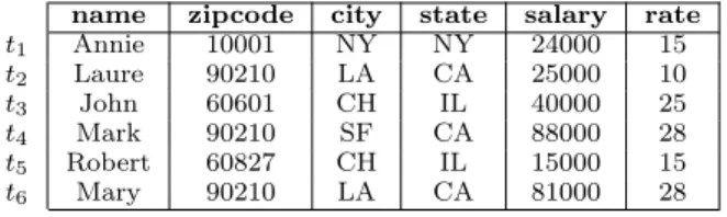
Example 1: Table 1 shows a sample tax data D in which each record represents an individual’s information. Suppose that the following three data quality rules need to hold on D: (r1) a zipcode uniquely determines a city; (r2) given two distinct individuals, the one earning a lower salary should have a lower tax rate; and (r3) two tuples refer to the same ∗
Partially done while at QCRI.
Permission to make digital or hard copies of all or part of this work for personal or classroom use is granted without fee provided that copies are not made or distributed for profit or commercial advantage and that copies bear this notice and the full citation on the first page. Copyrights for components of this work owned by others than ACM must be honored. Abstracting with credit is permitted. To copy otherwise, or republish, to post on servers or to redistribute to lists, requires prior specific permission and/or a fee. Request permissions from [email protected].
Copyright 20XX ACM X-XXXXX-XX-X/XX/XX ...$15.00.
name zipcode city state salary rate
t1 Annie 10001 NY NY 24000 15 t2 Laure 90210 LA CA 25000 10 t3 John 60601 CH IL 40000 25 t4 Mark 90210 SF CA 88000 28 t5 Robert 60827 CH IL 15000 15 t6 Mary 90210 LA CA 81000 28
Table 1: Dataset D with tax data records individual if they have similar names, and their cities are inside the same county. We define these rules as follows: (r1) φF : D(zipcode → city)
(r2) φD: ∀t1, t2∈ D, ¬(t1.rate > t2.rate ∧ t1.salary < t2.salary) (r3) φU: ∀t1, t2∈ D, ¬(simF(t1.name, t2.name)∧
getCounty(t1.city) = getCounty(t2.city))
φF, φD, and φU can respectively be expressed as a
func-tional dependency (FD), a denial constraint (DC), and a
user-defined function (UDF) by using a procedural language.
φU requires an ad-hoc similarity function and access to a
mapping table to get the county information. Tuples t2 and
t4form an error w.r.t. φF, so do t4and t6, because they have
the same zipcode but different city values. Tuples t1 and t2
violate φD, because t1 has a lower salary than t2 but pays
a higher tax; so do t2 and t5. Rule φU does not have data
errors, i.e., no duplicates in D w.r.t. φU. 2
Cleansing the above dataset typically consists of three steps: (1) specifying quality rules; (2) detecting data rors w.r.t. the specified rules; and (3) repairing detected er-rors. Generally speaking, after step (1), the data cleansing process iteratively runs steps (2) and (3) until obtaining an instance of the data (a.k.a. a repair) that satisfies the spec-ified rules. These three steps have been extensively studied in single-node settings [6, 7, 11, 16–18, 23, 34]. However, the main focus has been on how to more effectively detect and repair errors, without addressing the issue of scalability.
Dealing with large datasets faces two main issues. First, none of the existing systems can scale to large datasets for the rules in the example. One main reason is that detecting
errors, e.g., with φF and φD, or duplicates, e.g., with φU, is
a combinatorial problem that quickly becomes very expen-sive with large sizes. More specifically, if |D| is the number of tuples in a dataset D and n is the number of tuples a given rule is defined on (e.g., n = 2 for the above rules), the time
complexity of detecting errors is O(|D|n). This high
com-plexity leads to intractable computations over large datasets, limiting the applicability of data cleansing systems. For in-stance, memory-based approaches [6, 7] report performance numbers up to 100K tuples while a disk-based approach [17] reports numbers up to 1M records only. Apart from the scale problem, implementing such rules in a distributed
process-ing platform requires expertise both in the understandprocess-ing of the quality rules and in the tuning of their implementation over this platform. Some research efforts have targeted the usability of a data cleansing system (e.g., NADEEF [7]), but at the expense of performance and scalability.
Therefore, designing a distributed data cleansing system to deal with big data faces two main challenges:
(1) Scalability. Quality rules are varied and complex: they might compare multiple tuples, use similarity comparisons,
or contain inequality comparisons. Detecting errors in a
distributed setting may lead to shuffling large amounts of data through the network, with negative effects on the
per-formance. Moreover, existing repair algorithms were not
designed for distributed settings. For example, they often represent detected errors as a graph, where each node rep-resents a data value and an edge indicates a data error. De-vising algorithms on such a graph in distributed settings is not well addressed in the literature.
(2) Abstraction. In addition to supporting traditional
qual-ity rules (e.g., φF and φD), users also need the flexibility
to define rules using procedural programs (UDFs), such as
φU. However, effective parallelization is hard to achieve with
UDFs, since they are handled as black boxes. To enable scal-ability, finer granular constructs for specifying the rules are needed. An abstraction for this specification is challenging as it would normally come at the expense of generality of rule specification.
To address these challenges, we present BigDansing, a Big Data Cleansing system that is easy-to-use and highly scalable. It provides a rule specification abstraction that consists of five operators that allow users to specify data flows for error detection, which was not possible before. The internal rewriting of the rules enables effective optimiza-tions. In summary, we make the following contributions: (1) BigDansing abstracts the rule specification process into a logical plan composed of five operators, which it opti-mizes for efficient execution. Users focus on the logic of their rules, rather than on the details of efficiently implementing them on top of a parallel data processing platform. More importantly, this abstraction allows to detect errors and find possible fixes w.r.t. a large variety of rules that cannot be expressed in declarative languages (Section 3).
(2) BigDansing abstraction enables a number of optimiza-tions. We present techniques to translate a logical plan into an optimized physical plan, including: (i) removing data redundancy in input rules and reducing the number of oper-ator calls; (ii) specialized operoper-ators to speed up the cleansing process; and (iii) a new join algorithm, based on partitioning and sorting data, to efficiently perform distributed inequal-ity self joins (which are common in qualinequal-ity rules);
(3) We present two approaches to implement existing re-pair algorithms in distributed settings. First, we show how to run a centralized data repair algorithm in parallel, with-out changing the algorithm (Section 5.1). Second, we design a distributed version of the seminal equivalence class algo-rithm [5] (Section 5.2).
(4) We use both real-world and synthetic datasets to exten-sively validate our system. BigDansing outperforms base-line systems by up to more than two orders of magnitude. The results also show that BigDansing is more scalable than baseline systems without sacrificing the quality pro-vided by the repair algorithms (Section 6).
2.
FUNDAMENTALS AND AN OVERVIEW
We discuss the data cleansing semantics expressed by Big-Dansing and then give an overview of the system.
2.1
Data Cleansing Semantics
In BigDansing, the input data is defined as a set of data units, where each data unit is the smallest unit of input datasets. Each unit can have multiple associated elements that are identified by model-specific functions. For exam-ple, tuples are the data units for the relational model and attributes identify their elements, while triples are the data units for RDF data (see Appendix C). BigDansing provides a set of parsers for producing such data units and elements from input datasets.
BigDansing adopts UDFs as the basis to define quality rules. Each rule has two fundamental abstract functions,
namely Detect and GenFix. Detect takes one or multiple
data units as input and outputs a violation, i.e., elements in the input units that together are considered as erroneous w.r.t. the rule:
Detect(data units) → violation
GenFix takes a violation as input and computes alternative, possible updates to resolve this violation:
GenFix(violation) → possible fixes
The language of the possible fixes is determined by the
capabilities of the repair algorithm. With the supported
algorithms, a possible fix in BigDansing is an expression of the form x op y, where x is an element, op is in {=, 6=, <, >, ≥ , ≤}, and y is either an element or a constant. In addition, BigDansing has new functions to enable distributed and scalable execution of the entire cleansing process. We defer the details to Section 3.
Consider Example 1, the Detect function of φF takes two
tuples (i.e., two data units) as input and identifies a vio-lation whenever the same zipcode value appears in the two
tuples but with a different city. Thus, t2(90210, LA) and
t4(90210, SF ) are a violation. The GenFix function could
enforce either t2[city] and t4[city] to be the same, or at least
one element between t2[zipcode] and t4[zipcode] to be
differ-ent from 90210. Rule φUis more general as it requires special
processing. Detect takes two tuples as input and outputs a violation whenever it finds similar name values and obtains the same county values from a mapping table. GenFix could propose to assign the same values to both tuples so that one of them is removed in set semantics.
By using a UDF-based approach, we can support a large variety of traditional quality rules with a parser that
auto-matically implements the abstract functions, e.g.,CFDs[11]
and DCs [6], but also more procedural rules that are
pro-vided by the user. These latter rules can implement any de-tection and repair method expressible with procedural code, such as Java, as long as they implement the signatures of the two above functions, as demonstrated in systems such as NADEEF [7]. Note that one known limitation of UDF-based systems is that, when treating UDFs as black-boxes, it is hard to do static analysis, such as consistency and im-plication, for the given rules.
BigDansing targets the following data cleansing problem: given a dirty data D and a set of rules Σ, compute a repair
which is an updated instance D0 such that there are no
Figure 1: BigDansing architecture
Among the many possible solutions to the cleans-ing problem, it is common to define a notion of
min-imality based on the cost of a repair. A popular
cost function [5] for relational data is the following: P
t∈D,t0∈D
r,A∈ARdisA(D(t[A]), D(t
0
[A])), where t0is the fix
for a specific tuple t and disA(D(t[A]), D(t0[A])) is a distance
between their values for attribute A (an exact match returns 0). This models the intuition that the higher is the sum of the distances between the original values and their fixes, the more expensive is the repair. Computing such minimum
re-pairs is NP-hard, even with FDs only [5, 23]. Thus, data
repair algorithms are mostly heuristics (see Section 5).
2.2
Architecture
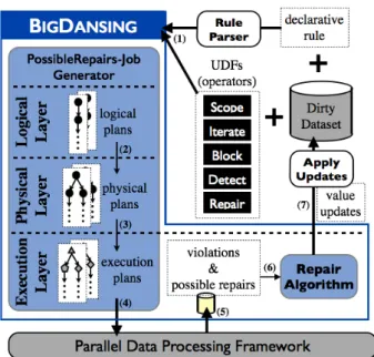
We architected BigDansing as illustrated in Figure 1. BigDansing receives a data quality rule together with a dirty dataset from users (1) and outputs a clean dataset (7). BigDansing consists of two main components: the RuleEngine and the RepairAlgorithm.
The RuleEngine receives a quality rule either in a UDF-based form (a BigDansing job) or in a declarative form (a declarative rule). A job (i.e., a script) defines users opera-tions as well as the sequence in which users want to run their operations (see Appendix A). A declarative rule is written
using traditional integrity constraints such asFDsandDCs.
In the latter case, the RuleEngine automatically translates the declarative rule into a job to be executed on a parallel data processing framework. This job outputs the set of vio-lations and possible fixes for each violation. The RuleEngine has three layers: the logical, physical, and execution layers. This architecture allows BigDansing to (i) support a large variety of data quality rules by abstracting the rule speci-fication process, (ii) achieve high efficiency when cleansing datasets by performing a number of physical optimizations, and (iii) scale to big datasets by fully leveraging the scala-bility of existing parallel data processing frameworks. No-tice that, unlike a DBMS, the RuleEngine also has an exe-cution abstraction, which allows BigDansing to run on top of general purpose data processing frameworks ranging from MapReduce-like systems to databases.
(1) Logical layer. A major goal of BigDansing is to allow users to express a variety of data quality rules in a simple way. This means that users should only care about the logic of their quality rules, without worrying about how to make the code distributed. To this end, BigDansing provides five logical operators, namely Scope, Block, Iterate, Detect, and GenFix, to express a data quality rule: Scope defines the rel-evant data for the rule; Block defines the group of data units among which a violation may occur; Iterate enumerates the candidate violations; Detect determines whether a candidate violation is indeed a violation; and GenFix generates a set of possible fixes for each violation. Users define these logi-cal operators, as well as the sequence in which BigDansing has to run them, in their jobs. Alternatively, users provide a declarative rule and BigDansing translates it into a job having these five logical operators. Notice that a job repre-sents the logical plan of a given input quality rule.
(2) Physical layer. In this layer, BigDansing receives a logical plan and transforms it into an optimized physical plan of physical operators. Like in DBMSs, a physical plan specifies how a logical plan is implemented. For example, Block could be implemented by either hash-based or range-based methods. A physical operator in BigDansing also contains extra information, such as the input dataset and the degree of parallelism. Overall, BigDansing processes a log-ical plan through two main optimization steps, namely the plan consolidation and the data access optimization, through the use of specialized join and data access operators. (3) Execution layer. In this layer, BigDansing determines how a physical plan will be actually executed on the under-lying parallel data processing framework. It transforms a physical plan into an execution plan which consists of a set of system-dependent operations, e.g., a Spark or MapReduce job. BigDansing runs the generated execution plan on the underlying system. Then, it collects all the violations and possible fixes produced by this execution. As a result, users get the benefits of parallel data processing frameworks by just providing few lines of code for the logical operators.
Once BigDansing has collected the set of violations and possible fixes, it proceeds to repair (cleanse) the input dirty dataset. At this point, the repair process is independent from the number of rules and their semantics, as the repair algorithm considers only the set of violations and their pos-sible fixes. The way the final fixes are chosen among all the possible ones strongly depends on the repair algorithm itself. Instead of proposing a new repair algorithm, we present in Section 5 two different approaches to implement existing algorithms in a distributed setting. Correctness and termi-nation properties of the original algorithms are preserved in our extensions. Alternatively, expert users can plug in their own repair algorithms. In the algorithms that we extend, each repair step greedily eliminates violations with possi-ble fixes while minimizing the cost function in Section 2.1. An iterative process, i.e., detection and repair, terminates if there are no more violations or there are only violations with no corresponding possible fixes. The repair step may introduce new violations on previously fixed data units and a new step may decide to again update these units. To en-sure termination, the algorithm put a special variable on such units after a fixed number of iterations (which is a user defined parameter), thus eliminating the possibility of future violations on the same data.
3.
RULE SPECIFICATION
BigDansing abstraction consists of five logical opera-tors: Scope, Block, Iterate, Detect, and GenFix, which are powerful enough to express a large spectrum of cleansing tasks. While Detect and GenFix are the two general oper-ators that model the data cleansing process, Scope, Block, and Iterate enable the efficient and scalable execution of that process. Generally speaking, Scope reduces the amount of data that has to be treated, Block reduces the search space for the candidate violation generation, and Iterate efficiently traverses the reduced search space to generate all candidate violations. It is worth noting that these five operators do not model the repair process itself (i.e., a repair algorithm). The system translates these operators along with a, generated or user-provided, BigDansing job into a logical plan.
3.1
Logical Operators
As mentioned earlier, BigDansing defines the input data through data units U s on which the logical operators oper-ate. While such a fine-granular model might seem to incur a high cost as BigDansing calls an operator for each U , it in fact allows to apply an operator in a highly parallel fashion. In the following, we define the five operators provided by BigDansing and illustrate them in Figure 2 using the
dataset and ruleFDφF (zipcode → city) of Example 1.
No-tice that the following listings are automatically generated by the system for declarative rules. Users can either modify this code or provide their own for the UDFs case.
(1) Scope removes irrelevant data units from a dataset. For each data unit U , Scope outputs a set of filtered data units, which can be an empty set.
Scope(U ) → listhU0i
Notice that Scope outputs a list of U s as it allows data units to be replicated. This operator is important as it allows BigDansing to focus only on data units that are relevant to a given rule. For instance, in Figure 2, Scope projects on attributes zipcode and city. Listing 4 (Appendix B) shows
the lines of code for Scope in rule φF.
(2) Block groups data units sharing the same blocking key. For each data unit U , Block outputs a blocking key.
Block(U ) → key
The Block operator is crucial for BigDansing’s scalability as it narrows down the number of data units on which a vi-olation might occur. For example, in Figure 2, Block groups tuples on attribute zipcode, resulting in three blocks, with each block having a distinct zipcode. Violations might occur inside these blocks only and not across blocks. See Listing 5 (Appendix B) for the single line of code required by this
operator fro rule φF.
(3) Iterate defines how to combine data units U s to gener-ate candidgener-ate violations. This operator takes as input a list of lists of data units U s (because it might take the output of several previous operators) and outputs a single U , a pair of U s, or a list of U s.
Iterate(listhlisthU ii) → U0 | hUi, Uji | listhU
00 i This operator allows to avoid the quadratic complexity for generating candidate violations. For instance, in Figure 2, Iterate passes each unique combination of two tuples inside each block, producing four pairs only (instead of 13 pairs):
(1) Scope (zipcode, city) (2) Block (zipcode) (3) Iterate (t3, t5) (t2, t4) (t2, t6) (t4, t6) (4) Detect (t2, t4) (t4, t6) zipcode city 10001 NY 90210 LA 60601 CH 90210 SF t1 t2 t3 t4 t5 60601 CH t6 90210 LA zipcode city 10001 NY 90210 SF 90210 LA t1 t4 60601 CH t3 t2 t5 60601 CH B1 B2 B3 LA 90210 t6 (5) GenFix t2[city] = t4[city]; t6[city] = t4[city]
Figure 2: Logical operators execution for ruleFDφF
(t3, t5) from B1, (t2, t4), (t2, t6), and (t4, t6) from B3.
List-ing 6 (Appendix B) shows the code required by this Iterate
operator for rule φF.
(4) Detect takes a single U , a pair-U , or a list o U s, as input and outputs a list of violations, possibly empty.
Detect(U | hUi, Uji | listhU0i) → {listhviolationi}
Considering three types of inputs for Detect allows us to achieve better parallelization by distinguishing between dif-ferent granularities of the input. For example, having 1K U s as input, rather than a single list of U s, would allow us to run 1K parallel instances of Detect (instead of a single Detect instance). In Figure 2, Detect outputs two violations,
v1 = (t2, t4) and v2= (t6, t4), as they have different values
for city; and it requires the lines of code in Listing 1. public ArrayList <Violation> detect(TuplePair in ) {
1 ArrayList <Violation> lst =newArrayList<Violation>(); 2 if (! in . getLeft () . getCellValue (1) . equals (
in . getRight() . getCellValue (1))) {
3 Violation v =newViolation(”zipcode => City”); 4 v.addTuple(in. getLeft () ) ;
5 v.addTuple(in. getRight() ) ;
6 lst . add(v); }
7 return lst ; }
Listing 1: Code example for the Detect operator. (5) GenFix computes a set of possible fixes for a given violation.
GenFix(violation) → {listhPossibleFixesi}
For instance, assuming that only right-hand side values can be modified, GenFix produces one possible repair for each
detected violation (Figure 2): t2[city] = t4[city] and t6[city] =
t4[city]. Listing 2 shows the code for this GenFix.
public ArrayList <Fix> GenFix(Violation v) { 1 ArrayList <Fix> result =newArrayList<Fix>(); 2 Tuple t1 = v.getLeft () ;
3 Tuple t2 = v.getRight() ;
4 Cell c1 =newCell(t1.getID() ,”City ”, t1 . getCellValue (1)) ; 5 Cell c2 =newCell(t2.getID() ,”City ”, t2 . getCellValue (1)) ; 6 result . add(newFix(c1,”=”,c2)) ;
7 return result ; }
Listing 2: Code example for the GenFix operator. Additionally, to better specify the data flow among the different operators, we introduce a label to stamp a data item and track how it is being processed.
In contrast to DBMS operators, BigDansing’s operators are UDFs, which allow users to plug in any logic. As a result, we are not restricted to a specific data model. However, for ease of explanations all of our examples assume relational
Detect Iterate Block Scope Rule Logical plan Found Not found Not found Found GenFix Not found Found Not found
Figure 3: Planner execution flow
data. We report an RDF data cleansing example in Ap-pendix C. We also report in ApAp-pendix D the code required to write the same rule in a distributed environment, such as Spark. The proposed templates for the operators allow users to get distributed detection without any expertise on Spark, only by providing from 3 to 16 lines of Java code. The benefit of the abstraction should be apparent at this point: (i) ease-of-use for non-expert users and (ii) better scalability thanks to its abstraction.
3.2
The Planning Process
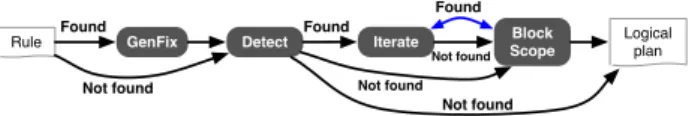
The logical layer of BigDansing takes as input a set of labeled logical operators together with a job and outputs a logical plan. The system starts by validating whether the provided job is correct by checking that all referenced logi-cal operators are defined and at least one Detect is specified.
Recall that for declarative rules, such as CFDs and DCs,
users do not need to provide any job, as BigDansing auto-matically generates a job along with the logical operators.
After validating the provided job, BigDansing generates a logical plan (Figure 3) that: (i) must have at least one
input dataset Di; (ii) may have one or more Scope
opera-tors; (iii) may have one Block operator or more linked to an Iterate operator; (iv) must have at least one Detect operator to possibly produce a set of violations; and (v) may have one GenFix operator for each Detect operator to generate possible fixes for each violation.
BigDansing looks for a corresponding Iterate operator for each Detect. If Iterate is not specified, BigDansing gener-ates one according to the input required by the Detect op-erator. Then, it looks for Block and Scope operators that match the input label of the Detect operator. If an Iterate operator is specified, BigDansing identifies all Block oper-ators whose input label match the input label of the Iterate. Then, it uses the input labels of the Iterate operator to find other possible Iterate operators in reverse order. Each new detected Iterate operator is added to the plan with the Block operators related to its input labels. Once it has processed all Iterate operators, it finally looks for Scope operators.
In case the Scope or Block operators are missing, Big-Dansing pushes the input dataset to the next operator in the logical plan. If no GenFix operator is provided, the out-put of the Detect operator is written to disk. For example, assume the logical plan in Figure 4, which is generated by BigDansing when a user provides the job in Appendix A. We observe that dataset D1 is sent directly to a Scope and a Block operator. Similarly, dataset D2 is sent directly to an Iterate operator. We also observe that one can also iterate over the output of previous Iterate operators (e.g., over
out-put DM). This flexibility allows users to express complex
data quality rules, such as in the form of “bushy” plans as shown in Appendix E.
4.
BUILDING PHYSICAL PLANS
When translating a logical plan, BigDansing exploits two main opportunities to derive an optimized physical plan: (i) static analysis of the logical plan and (ii) alternative translations for each logical operator. Since quality rules
Scope Block D1 S Block S T Iterate S T Iterate D2 M W Detect V GenFix V
Figure 4: Example of a logical plan
may involve joins over ordering comparisons, we also intro-duce an efficient algorithm for these cases. We discuss these aspects in this section. In addition, we discuss data storage and access issues in Appendix F.
4.1
Physical Operators
There are two kinds of physical operators: wrappers and
enhancers. A wrapper simply invokes a logical operator.
Enhancers replace wrappers to take advantage of different optimization opportunities.
A wrapper invokes a logical operator together with the cor-responding physical details, e.g., input dataset and schema details (if available). For clarity, we discard such physical details in all the definitions below. In contrast to the logical layer, BigDansing invokes a physical operator for a set D of data units, rather than for a single unit. This enables the processing of multiple units in a single function call. For each logical operator, we define a corresponding wrapper. (1) PScope applies a user-defined selection and projection
over a set of data units D and outputs a dataset D0⊂ D.
PScope(D) → {D0}
(2) PBlock takes a dataset D as input and outputs a list of key-value pairs defined by users.
PBlock(D) → maphkey, listhU ii
(3) PIterate takes a list of lists of U s as input and outputs their cross product or a user-defined combination.
PIterate(listhlisthU ii) → listhU i | listhPairhU ii (4) PDetect receives either a list of data units U s or a list of data unit pairs U -pairs and produces a list of violations.
PDetect(listhU i | listhPairhU ii) → listhV iolationi (5) PGenFix receives a list of violations as input and out-puts a list of a set of possible fixes, where each set of fixes belongs to a different input violation.
PGenFix(listhV iolationi) → listh{P ossibleF ixes}i With declarative rules, the operations over a dataset are known, which enables algorithmic opportunities to improve performance. Notice that one could also discover such oper-ations with code analysis over the UDFs [20]. However, we leave this extension to future work. BigDansing exploits such optimization opportunities via three new enhancers op-erators: CoBlock, UCrossProduct, and OCJoin. CoBlock is a physical operator that allows to group multiple datasets by a given key. UCrossProduct and OCJoin are basically two additional different implementations for the PIterate opera-tor. We further explain these three enhancers operators in the next section.
Algorithm 1: Logical plan consolidation input : LogicalPlan lp
output: LogicalPlan clp
1 PlanBuilder lpb = new PlanBuilder();
2 for logical operator lopi ∈ lp do
3 lopj ← findMatchingLO(lopi, lp);
4 DS1 ← getSourceDS(lopi);
5 DS2 ← getSourceDS(lopj);
6 if DS1 == DS2 then
7 lopc ← getLabelsFuncs(lopi, lopj);
8 lopc.setInput(DS1, DS2); 9 lpb.add(lopc); 10 lp.remove(lopi, lopj); 11 if lpb.hasConsolidatedOps then 12 lpb.add(lp.getOperators()); 13 return lpb.generateConsolidatedLP(); 14 else 15 return lp;
4.2
From Logical to Physical Plan
As we mentioned earlier, optimizing a logical plan is per-formed by static analysis (plan consolidation) and by plug-ging enhancers (operators translation) whenever possible.
Plan Consolidation. Whenever logical operators use a
different label for the same dataset, BigDansing translates them into distinct physical operators. BigDansing has to create multiple copies of the same dataset, which it might broadcast to multiple nodes. Thus, both the memory foot-print at compute nodes and the network traffic are increased. To address this problem, BigDansing consolidates redun-dant logical operators into a single logical operator. Hence, by applying the same logical operator several times on the same set of data units using shared scans, BigDansing is able to increase data locality and reduce I/O overhead.
Algorithm 1 details the consolidation process for an input
logical plan lp. For each operator lopi, the algorithm looks
for a matching operator lopj (Lines 2-3). If lopj has the
same input dataset as lopi, BigDansing consolidates them
into lopc(Lines 4-6). The newly consolidated operator lopc
takes the labels, functions, and datasets from lopiand lopj
(Lines 7-8). Next, BigDansing adds lopcinto a logical plan
builder lpb and removes lopi and lopj from lp (Lines 9-10).
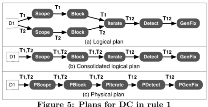
At last, if any operator was consolidated, it adds the non-consolidated operators to lpb and returns the non-consolidated logical plan (Lines 11-13). Otherwise, it returns lp (Line 15). Let us now illustrate the consolidation process with an example. Consider a DC on the TPC-H database stating that if a customer and a supplier have the same name and phone they must be in the same city. Formally,
DC : ∀t1, t2 ∈ D1, ¬(t1.c name = t2.s name∧
t1.c phone = t2.s phone ∧ t1.c city 6= t2.s city)
(1) For this DC, BigDansing generates the logical plan in Fig-ure 5(a) with operators Scope and Block applied twice over the same input dataset. It then consolidates redundant log-ical operators into a single one (Figure 5(b)) thereby reduc-ing the overhead of readreduc-ing an input dataset multiple times. The logical plan consolidation is only applied when it does not affect the original labeling of the operators.
Operators Translation. Once a logical plan have been consolidated, BigDansing translates the consolidated
logi-Scope Block D1 T1 Iterate Detect Scope T2 Block T1 T1 T2 T 2 T12
(a) Logical plan
Scope Block
D1 IterateT12 Detect
T1,T2
(b) Consolidated logical plan
PScope PBlock D1 PIterate PDetect T12 (c) Physical plan T1,T2 T1,T2 T1,T2 T1,T2 T1,T2 GenFix T12 GenFix T12 PGenFix T12
Figure 5: Plans for DC in rule 1
cal plan into a physical plan. It maps each logical operator to its corresponding wrapper, which in turn maps to one or more physical operators. For example, it produces the phys-ical plan in Figure 5(c) for the consolidated logphys-ical plan in Figure 5(b). For enhancers, BigDansing exploits some par-ticular information from the data cleansing process. Below, we detail these three enhancers operators as well as in which cases they are used by our system.
• CoBlock takes multiple input datasets D and applies a group-by on a given key. This would limit the comparisons required by the rule to only blocks with the same key from the different datasets. An example is shown in Figure 16 (Appendix E). Similar to the CoGroup defined in [28], in the output of CoBlock, all keys from both inputs are collected into bags. The output of this operator is a map from a key value to the list of data units sharing that key value. We formally define this operator as:
CoBlock (D) → maphkey, listhlisthU iii
If two non-consolidated Block operators’ outputs go to the same Iterate and then to a single PDetect, BigDansing translates them into a single CoBlock. Using CoBlock al-lows us to reduce the number of candidate violations for the Detect. This is because Iterate generates candidates only inside and not across CoBlocks (see Figure 6).
• UCrossProduct receives a single input dataset D and ap-plies a self cross product over it. This operation is usually performed in cleansing processes that would output the same violations irrespective of the order of the input of Detect. UCrossProduct avoids redundant comparisons, reducing the
number of comparisons from n2 to n×(n−1)
2 , with n being
the number of units U s in the input. For example, the out-put of the logical operator Iterate in Figure 2 is the result of UCrossProduct within each block; there are four pairs in-stead of thirteen, since the operator avoids three compar-isons for the elements in block B1 and six for the ones in B3 of Figure 2. Formally:
UCrossProduct(D) → listhPairhU ii
If, for a single dataset, the declarative rules contain only symmetric comparisons, e.g., = and 6=, then the order in which the tuples are passed to PDetect (or to the next logical operator if any) does not matter. In this case, BigDansing uses UCrossProduct to avoid materializing many unnecessary pairs of data units, such as for the Iterate operator in Fig-ure 2. It also uses UCrossProduct when: (i) users do not provide a matching Block operator for the Iterate operator; or (ii) users do not provide any Iterate or Block operator. • OCJoins performs a self join on one or more ordering com-parisons (i.e., <, >, ≥, ≤). This is a very common operation
Scope1 Block1 D1 T1 Iterate Detect Scope2 T2 Block2 T1 T1 T2 T 2 T12
(a) Logical plan with non-consolidated Block operators
(b) Physical plan GenFix T12 PScope1 D1 T 1 PIterate PDetect PScope2 T2 CoBlock T1 T2 T12 PGenFix T12 T12 D2 D2
Figure 6: Example plans with CoBlock in rules such as DCs. Thus, BigDansing provides OCJoin, which is an efficient operator to deal with join ordering com-parisons. It takes input dataset D and applies a number of join conditions, returning a list of joining U -pairs. We for-mally define this operator as follows:
OCJoin(D) → listhPairhU ii
Every time BigDansing recognizes joins conditions defined
with ordering comparisons in PDetect, e.g., φD, it
trans-lates Iterate into a OCJoin implementation. Then, it passes OCJoin output to a PDetect operator (or to the next logi-cal operator if any). We discuss this operator in detail in Section 4.3.
We report details for the transformation of the physical operators to two distributed platforms in Appendix G.
4.3
Fast Joins with Ordering Comparisons
Existing systems handle joins over ordering comparisons using a cross product and a post-selection predicate, leading to poor performance. BigDansing provides an efficient ad-hoc join operator, referred to as OCJoin, to handle these cases. The main goal of OCJoin is to increase the ability to process joins over ordering comparisons in parallel and to reduce its complexity by reducing the algorithm’s search space. In a nutshell, OCJoin first range partitions a set of data units and sorts each of the resulting partitions in order to validate the inequality join conditions in a distributed fashion. OCJoin works in four main phases: partitioning, sorting, pruning, and joining (see Algorithm 2).
Partitioning. OCJoin first selects the attribute, P artAtt,
on which to partition the input D (line 1). We assume
that all join conditions have the same output cardinality. This can be improved using cardinality estimation tech-niques [9,27], but it is beyond the scope of the paper. OCJoin chooses the first attribute involved in the first condition.
For instance, consider again φD (Example 1), OCJoin sets
P artAtt to rate attribute. Then, OCJoin partitions the input dataset D into nbP arts range partitions based on P artAtt
(line 2). As part of this partitioning, OCJoin distributes
the resulting partitions across all available computing nodes. Notice that OCJoin runs the range partitioning in parallel. Next, OCJoin forks a parallel process for each range partition
kito run the three remaining phases (lines 3-14).
Sorting. For each partition, OCJoin creates as many sorting lists (Sorts) as inequality conditions are in a rule (lines
4-5). For example, OCJoin creates two sorted lists for φD:
one sorted on rate and the other sorted on salary. Each
list contains the attribute values on which the sort order is and the tuple identifiers. Note that OCJoin only performs a local sorting in this phase and hence it does not require any data transfer across nodes. Since multiple copies of a
Algorithm 2: OCJoin
input : Dataset D, Condition conds[ ], Integer nbParts output: List TupleshTuplei
// Partitioning Phase
1 PartAtt ← getPrimaryAtt(conds[].getAttribute());
2 K ← RangePartition(D, PartAtt, nbParts);
3 for each ki∈ K do
4 for each cj∈ conds[ ] do // Sorting
5 Sorts[j] ← sort(ki, cj.getAttribute());
6 for each kl∈ {ki+1...k|K|} do
7 if overlap(ki, kl, PartAtt) then // Pruning
8 tuples = ∅;
9 for each cj∈ conds[ ] do // Joining
10 tuples ← join(ki, kl, Sorts[j], tuples);
11 if tuples == ∅ then
12 break;
13 if tuples != ∅ then
14 Tuples.add(tuples);
partition may exist in multiple computing nodes, we apply sorting before pruning and joining phases to ensure that each partition is sorted at most once.
Pruning. Once all partitions ki∈ K are internally sorted,
OCJoin can start joining each of these partitions based on the inequality join conditions. However, this would require transferring large amounts of data from one node to
an-other. To circumvent such an overhead, OCJoin inspects
the min and max values of each partition to avoid joining partitions that do not overlap in their min and max range (the pruning phase, line 7). Non-overlapping partitions do not produce any join result. If the selectivity values for the different inequality conditions are known, OCJoin can order the different joins accordingly.
Joining. OCJoin finally proceeds to join the overlapping partitions and outputs the join results (lines 9-14). For this, it applies a distributed sort merge join over the sorted lists, where some partitions are broadcast to other machines while keeping the rest locally. Through pruning, OCJoin tells the underlying distributed processing platform which partitions to join. It is up to that platform to select the best approach to minimize the number of broadcast partitions.
5.
DISTRIBUTED REPAIR ALGORITHMS
Most of the existing repair techniques [5–7, 11, 17, 23, 34] are centralized. We present two approaches to implement a repair algorithm in BigDansing. First, we show how our system can run a centralized data repair algorithm in par-allel, without changing the algorithm. In other words, Big-Dansing treats that algorithm as a black box (Section 5.1). Second, we design a distributed version of the widely used equivalence class algorithm [5, 7, 11, 17] (Section 5.2).
5.1
Scaling Data Repair as a Black Box
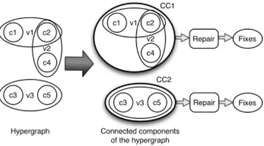
Overall, we divide a repair task into independent smaller repair tasks. For this, we represent the violation graph as a hypergraph containing the violations and their possible fixes. The nodes represent the elements and each hyperedge covers a set of elements that together violate a rule, along with possible repairs. We then divide the hypergraph into smaller independent subgraphs, i.e., connected components,
v3 v3 v1 c1 v2 c2 c4 c3 c5 v1 c1 v2 c2 c4 c3 c5 CC1 CC2 Fixes Fixes
Hypergraph Connected components of the hypergraph
Repair
Repair
Figure 7: Data repair as a black box. and we pass each connected component to an independent data repair instance.
Connected components. Given an input set of violations, form at least one rule, BigDansing first creates their hyper-graph representation of such possible fixes in a distributed manner. It then uses GraphX [37] to find all connected com-ponents in the hypergraph. GraphX, in turn, uses the Bulk Synchronous Parallel (BSP) graph processing model [25] to process the hypergraph in parallel. As a result, BigDans-ing gets a connected component ID for each hyperedge. It then groups hyperedges by the connected component ID. Figure 7 shows an example of connected components in a hypergraph containing three violations v1, v2, and v3. Note that violations v1 and v2 can be caused by different rules. Violations v1 and v2 are grouped in a single connected com-ponent CC1, because they share element c2. In contrast, v3 is assigned to a different connected component CC2, because it does not share any element with v1 or v2.
Independent data repair instance. Once all connected components are computed, BigDansing assigns each of them to an independent data repair instance and runs such repair instances in a distributed manner (right-side of Fig-ure 7). When all data repair instances generate the required fixes, BigDansing updates the input dataset and pass it again to the RuleEngine to detect potential violations in-troduced by the RepairAlgorithm. The number of iterations required to fix all violations depends on the input rules, the dataset, and the repair algorithm.
Dealing with big connected components. If a
con-nected component does not fit in memory, BigDansing uses a k-way multilevel hypergraph partitioning algorithm [22] to divide it into k equal parts and run them on distinct ma-chines. Unfortunately, naively performing this process can lead to inconsistencies and contradictory choices in the re-pair. Moreover, it can fix the same violation independently in two machines, thus introducing unnecessary changes to the repair. We illustrate this problem with an example. Example 2: Consider a relational schema D with 3 attributes
A, B, C and 2FDsA → B and C → B. Given the instance
[t1](a1, b1, c1), [t2](a1, b2, c1), all data values are in
viola-tion: t1.A, t1.B, t2.A, t2.B for the first FD and t1.B, t1.C,
t2.B, t2.C for the second one. Assuming the compute nodes
have enough memory only for five values, we need to solve the violations by executing two instances of the algorithm on two different nodes. Regardless of the selected tuple, sup-pose the first compute node repairs a value on attribute A, and the second one a value on attribute C. When we put the two repairs together and check their consistency, the updated instance is a valid solution, but the repair is not minimal because a single update on attribute B would have
solved both violations. However, if the first node fixes t1.B
by assigning value “b2” and the second one fixes t2.B with
“b1”, not only there are two changes, but the final instance
is also inconsistent. 2
We tackle the above problem by assigning the role of mas-ter to one machine and the role of slave to the rest. Every machine applies a repair in isolation, but we introduce an extra test in the union of the results. For the violations that are solved by the master, we mark its changes as immutable, which prevents us to change an element more than once. If a change proposed by a slave contradicts a possible repair that involve a master’s change, the slave repair is undone and a new iteration is triggered. As a result, the algorithm always reaches a fix point to produce a clean dataset, because an updated value cannot change in the following iterations.
BigDansing currently provides two repair algorithms us-ing this approach: the equivalence class algorithm and a general hypergraph-based algorithm [6, 23]. Users can also implement their own repair algorithm if it is compatible with BigDansing’s repair interface.
5.2
Scalable Equivalence Class Algorithm
The idea of the equivalence class based algorithm [5] is to first group all elements that should be equivalent together, and to then decide how to assign values to each group. An equivalence class consists of pairs of the form (t, A), where t is a data unit and A is an element. In a dataset D, each unit t and each element A in t have an associated equivalence class, denoted by eq(t, A). In a repair, a unique target value is assigned to each equivalence class E, denoted by targ(E). That is, for all (t, A) ∈ E, t[A] has the same value targ(E). The algorithm selects the target value for each equivalence class to obtain a repair with the minimum overall cost.
We extend the equivalence class algorithm to a distributed setting by modeling it as a distributed word counting al-gorithm based on map and reduce functions. However, in contrast to a standard word count algorithm, we use two map-reduce sequences. The first map function maps the vi-olations’ possible fixes for each connected component into key-value pairs of the form hhccID,valuei,counti. The key hccID,valuei is a composite key that contains the connected component ID and the element value for each possible fix. The value count represents the frequency of the element value, which we initialize to 1. The first reduce function counts the occurrences of the key-value pairs that share the same connected component ID and element value. It out-puts key-value pairs of the form hhccID,valuei,counti. Note that if an element exists in multiple fixes, we only count its value once. After this first map-reduce sequence, another map function takes the output of the reduce function to cre-ate new key-value pairs of the form hccID,hvalue,countii. The key is the connected component ID and the value is the frequency of each element value. The last reduce selects the element value with the highest frequency to be assigned to all the elements in the connected component ccID.
6.
EXPERIMENTAL STUDY
We evaluate BigDansing using both real and synthetic
datasets with various rules (Section 6.1). We consider a
variety of scenarios to evaluate the system and answer the following questions: (i) how well does it perform compared with baseline systems in a single node setting (Section 6.2)? (ii) how well does it scale to different dataset sizes compared to the state-of-the-art distributed systems (Section 6.3)? (iii) how well does it scale in terms of the number of nodes
Dataset Rows Dataset Rows
T axA1–T axA5 100K – 40M customer2 32M
T axB1–T axB3 100K – 3M NCVoter 9M
T P CH1–T P CH10 100K – 1907M HAI 166k
customer1 19M
Table 2: Statistics of the datasets
Identifier Rule
ϕ1 (FD): Zipcode → City
ϕ2 (DC): ∀t1, t2 ∈ T axB, ¬(t1.Salary > t2.Salary
∧t1.Rate < t2.Rate)
ϕ3 (FD): o custkey → c address
ϕ4 (UDF): Two rows in Customer are duplicates
ϕ5 (UDF): Two rows in NCVoter are duplicates
ϕ6 (FD): Zipcode → State
ϕ7 (FD): PhoneNumber → Zipcode
ϕ8 (FD): ProviderID → City, PhoneNumber
Table 3: Integrity constraints used for testing (Section 6.4)? (iv) how well does its abstraction support a variety of data cleansing tasks, e.g., for deduplication (Sec-tion 6.5)? and (v) how do its different techniques improve performance and what is its repair accuracy (Section 6.6)?
6.1
Setup
Table 2 summarizes the datasets and Table 3 shows the rules we use for our experiments.
(1) TaxA. Represents personal tax information in the US [11]. Each row contains a person’s name, contact in-formation, and tax information. For this dataset, we use
the FD rule ϕ1 in Table 3. We introduced errors by adding
random text to attributes City and State at a 10% rate. (2) TaxB. We generate TaxB by adding 10% numerical ran-dom errors on the Rate attribute of TaxA. Our goal is to validate the efficiency with rules that have inequality
condi-tions only, such asDCϕ2 in Table 3.
(3) TPCH. From the TPC-H benchmark data [2], we joined the lineitem and customer tables and applied 10% random
errors on the address. We use this dataset to testFDrule ϕ3.
(4) Customer. In our deduplication experiment, we use
TPC-H customer with 4.5 million rows to generate tables customer1 with 3x exact duplicates and customer2 with 5x exact duplicates. Then, we randomly select 20% of the total number of tuples, in both relations, and duplicate them with random edits on attributes name and phone.
(5) NCVoter. This is a real dataset that contains North Car-olina voter information. We added 20% random duplicate rows with random edits in name and phone attributes.
(6) Healthcare Associated Infections (HAI)
(http://www.hospitalcompare.hhs.gov). This real dataset
contains hospital information and statistics measurements for infections developed during treatment. We added 10%
random errors on the attributes covered by the FDs and
tested four combinations of rules (ϕ6 – ϕ8 from Table 3).
Each rule combination has its own dirty dataset.
To our knowledge, there exists only one full-fledged data cleansing system that can support all the rules in Table 3: (1) NADEEF [7]: An open-source single-node platform sup-porting both declarative and user defined quality rules. (2) PostgreSQL v9.3: Since declarative quality rules can be represented as SQL queries, we also compare to PostgreSQL
for violation detection. To maximize benefits from large
main memory, we configured it using pgtune [30].
0 500 1000 1500 2000 100K 1M 100K 200K 100K 1M R untime (Seconds) Number of rows BigDansing 14 30 165 NADEEF 36 160 951 19 121 31 Rule φ3 Rule φ2 Rule φ1
(a) Rules ϕ1, ϕ2, and ϕ3.
0 20 40 60 80 100 1% 5% 10% 50% Time (Seconds) Error percentage Violation detection Data repair (b) Rule ϕ1.
Figure 8: Data cleansing times.
The two declarative constraints, DC ϕ2 and FDϕ3 in
Ta-ble 3, are translated to SQL as shown below. ϕ2: SELECT a.Salary, b.Salary, a.Rate, b.Rate
FROM TaxB a JOIN TaxB b
WHERE a.Salary > b.Salary AND a.Rate < b.Rate;
ϕ3: SELECT a.o custkey, a.c address, b.c address FROM
TPCH a JOIN TPCH b ON a.custkey = b.custkey WHERE a.c address 6= b.c address;
We also consider two parallel data processing frameworks: (3) Shark 0.8.0 [38]: This is a scalable data processing en-gine for fast data analysis. We selected Shark due to its scalability advantage over existing distributed SQL engines. (4) Spark SQL v1.0.2:It is an experimental extension of Spark v1.0 that allows users run relational queries natively on Spark using SQL or HiveQL. We selected this system as, like BigDansing, it runs natively on top of Spark.
We ran our experiments in two different settings: (i) a single-node setting using a Dell Precision T7500 with two 64-bit quad-core Intel Xeon X5550 (8 physical cores and 16 CPU threads) and 58GB RAM and (ii) a multi-node setting using a compute cluster of 17 Shuttle SH55J2 machines (1 master with 16 workers) equipped with Intel i5 processors with 16GB RAM constructed as a star network.
6.2
Single-Node Experiments
For these experiments, we start comparing BigDansing with NADEEF in the execution times of the whole cleans-ing process (i.e., detection and repair). Figure 8(a) shows the performance of both systems using the TaxA and TPCH
datasets with 100K and 1M (200K for ϕ2) rows. We observe
that BigDansing is more than three orders of magnitude
faster than NADEEF in rules ϕ1 (1M) and ϕ2 (200K), and
ϕ3 (1M). In fact, NADEEF is only “competitive” in rule ϕ1
(100K), where BigDansing is only twice faster. The high superiority of BigDansing comes from two main reasons: (i) In contrast to NADEEF, it provides a finer granular ab-straction allowing users to specify rules more efficiently; and (ii) It performs rules with inequality conditions in an efficient way (using OCJoin). In addition, NADEEF issues thou-sands of SQL queries to the underlying DBMS. for detect-ing violations. We do not report results for larger datasets because NADEEF was not able to run the repair process for
more than 1M rows (300K for ϕ2).
We also observed that violation detection was dominating the entire data cleansing process. Thus, we ran an
exper-iment for rule ϕ1 in TaxA with 1M rows by varying the
error rate. Violation detection takes more than 90% of the time, regardless of the error rate (Figure 8(b)). In particu-lar, we observe that even for a very high error rate (50%), the violation detection phase still dominates the cleansing process. Notice that for more complex rules, such as rule
ampli-0 1000 2000 3000 4000 5000 6000 100,000 1,000,000 10,000,000 Runtime (Sec onds)
Dataset size (rows) BigDansing NADEEF PostgreSQL Spark SQL Shark 5 55 0.264 18 368 37 86 3183 4 2 8 47 80 4153
(a) TaxA data with ϕ1
0 2000 4000 6000 8000 10000 12000 14000 16000 100,000 200,000 300,000 Runtime (Sec onds)
Dataset size (rows) BigDansing NADEEF PostgreSQL Spark SQL Shark 10 833 30 62 4529 9336 2133 8780 3731 7982
(b) TaxB data with ϕ2
0 500 1000 1500 2000 100,000 1,000,000 10,000,000 Runtime (Sec onds)
Dataset size (rows) BigDansing NADEEF PostgreSQL Spark SQL Shark 6 34 10 140 423 2 29 377 5 7 8 47 44 562 (c) TPCH data with ϕ3
Figure 9: Single-node experiments with ϕ1, ϕ2, and ϕ1
0 5000 10000 15000 20000 10M 20M 40M T ime (Seconds)
Dataset size (rows) BigDansing-Spark BigDansing-Hadoop Spark SQL Shark 121 503 150 865 337 2302 159 313 662 3739 14113 126822
(a) TaxA data with ϕ1
0 20000 40000 60000 80000 100000 120000 1M 2M 3M T ime (Seconds)
Dataset size (rows) BigDansing-Spark Spark SQL Shark
1240 5319 7730
(b) TaxB data with ϕ2
0 40000 80000 120000 160000 200000 647M 959M 1271M1583M1907M T ime (Seconds)
Dataset size (rows) BigDansing-Spark BigDansing-Hadoop Spark SQL 712 24803 2307 52886 5113 8670 11880 92236 138932 196133 9263 17872 30195 46907 65115 (c) Large TPCH on ϕ3
Figure 10: Multi-nodes experiments with ϕ1, ϕ2 and ϕ3
fied. Therefore, to be able to extensively evaluate BigDans-ing, we continue our experiments focusing on the violation detection phase only, except if stated otherwise.
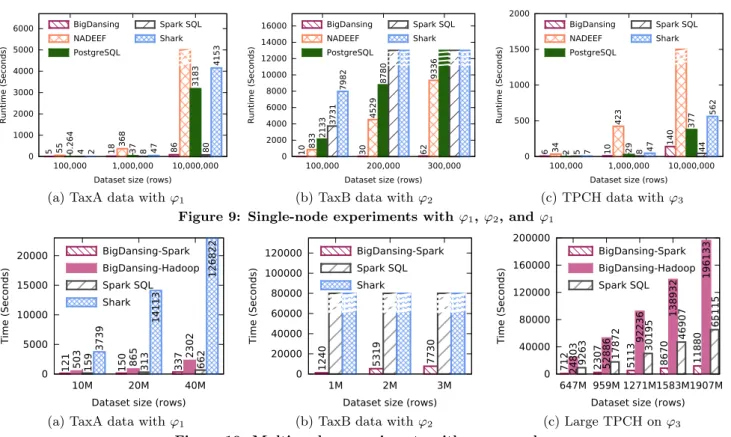
Figures 9(a), Figure 9(b), and 9(c) show the violation detection performance of all systems for TaxA, TaxB, and TPCH datasets. TaxA and TPCH datasets have 100K, 1M, and 10M rows and TaxB has 100K, 200K, and 300K rows.
With equality-based rules ϕ1and ϕ3, we observe that
Post-greSQL is always faster than all other systems on the small datasets (100K rows). However, once we increase the size by one order of magnitude (1M rows), we notice the advantage of BigDansing: it is at least twice faster than PostgreSQL and more than one order of magnitude faster than NADEEF. For the largest dataset (10M rows), BigDansing is almost
two orders of magnitude faster than PostgreSQL for theFD
in TaxA and one order of magnitude faster than PostgreSQL
for theDCin TaxA. For the FDin TPCH, BigDansing is
twice faster than PostgreSQL. It is more than three orders of magnitude faster than NADEEF for all rules. Overall, we observe that BigDansing performs similarly to Spark SQL. The small difference is that Spark SQL uses multithreading better than BigDansing. We can explain the superiority of BigDansing compared to the other systems along two reasons: (i) BigDansing reads the input dataset only once, while PostgreSQL and Shark read it twice because of the self joins; and (ii) BigDansing does not generate duplicate violations, while SQL engines do when comparing tuples
us-ing self-joins, such as for TaxA and TPCH’sFD. Concerning
the inequality-based rule ϕ2, we limited the runtime to four
hours for all systems. BigDansing is one order of magni-tude faster than all other systems for 100K rows. For 200K and 300K rows, it is at least two orders of magnitude faster than all baseline systems. Such performance superiority is achieved by leveraging the inequality join optimization that
is not supported by the baseline systems.
6.3
Multi-Node Experiments
We now compare BigDansing with Spark SQL and Shark in the multi-node setting. We also implemented a lighter version of BigDansing on top of Hadoop MapReduce to
show BigDansing independence w.r.t. the underlying
framework. We set the size of TaxA to 10M, 20M, and 40M
rows. Moreover, we tested the inequality DC ϕ2 on TaxB
dataset with sizes of 1M, 2M, and 3M rows. We limited the runtime to 40 hours for all systems.
BigDansing-Spark is slightly faster than Spark SQL for the equality rules in Figure 10(a). Even though BigDans-ing-Spark and Shark are both implemented on top of Spark, BigDansing-Spark is up to three orders of magnitude faster than Shark. Even BigDansing-Hadoop is doing better than Shark (Figure 10(a)). This is because Shark does not pro-cess joins efficiently. The performance of BigDansing over baseline systems is magnified when dealing with inequalities. We observe that BigDansing-Spark is at least two orders of magnitude faster than both Spark SQL and Shark (Fig-ure 10(b)). We had to stop Spark SQL and Shark executions after 40 hours of runtime; both Spark SQL and Shark are
unable to process the inequalityDCefficiently.
We also included a testing for large TPCH datasets of sizes 150GB, 200GB, 250GB, and 300GB (959M, 1271M, 1583M, and 1907M rows resp.) producing between 6.9B and 13B violations. We excluded Shark as it could not run on these larger datasets. BigDansing-Spark is 16 to 22 times faster than BigDansing-Hadoop and 6 to 8 times faster than Spark SQL (Figure 10(c)). BigDansing-Spark signifi-cantly outperforms Spark SQL since it has a lower I/O com-plexity and an optimized data cleansing physical execution plan. Moreover, the performance difference between Big-Dansing-Spark and BigDansing-Hadoop stems from Spark
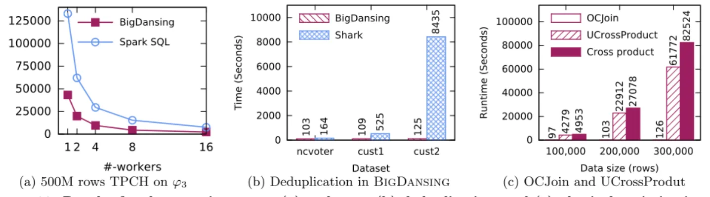
0 25000 50000 75000 100000 125000 1 2 4 8 16 R untime (Sec onds) #-workers BigDansing Spark SQL (a) 500M rows TPCH on ϕ3 0 2000 4000 6000 8000 10000
ncvoter cust1 cust2
Time (Seconds) Dataset BigDansing Shark 103 164 109 525 125 8435 (b) Deduplication in BigDansing 0 20000 40000 60000 80000 100000 100,000 200,000 300,000 Runtime (Seconds)
Data size (rows) OCJoin UCrossProduct Cross product 97 4279 103 126 22912 61772 4953 27078 82524
(c) OCJoin and UCrossProdut Figure 11: Results for the experiments on (a) scale-out, (b) deduplication, and (c) physical optimizations. being generally faster than Hadoop; Spark is an in-memory
data processing system while Hadoop is disk-based.
6.4
Scaling BigDansing Out
We compared the speedup of BigDansing-Spark to Spark SQL when increasing the number of workers on a dataset size of 500M rows. We observe that BigDansing-Spark is at least 3 times faster than BigDansing-Spark SQL starting from one single worker and up to 16 (Figure 11(a)). We also notice that BigDansing-Spark is about 1.5 times faster than Spark SQL while using only half the number of work-ers used by Spark SQL. Although both BigDansing-Spark and Spark SQL generally have a good scalability, BigDans-ing-Spark performs better than Spark SQL on large input datasets since it does not copy the input data twice.
6.5
Deduplication in BigDansing
We show that one can run a deduplication task with Big-Dansing. We use cust1, cust2, and NCVoters datasets on
our compute cluster. We implemented a Java version of
Levenshtein distance and use it as a UDF in both BigDans-ing and Shark. Note that we do not consider Spark SQL in this experiment since UDFs cannot be implemented di-rectly within Spark SQL. That is, to implement a UDF in Spark SQL the user has to either use a Hive interface or ap-ply a post processing step on the query result. Figure 11(b) shows the results. We observe that BigDansing outper-forms Shark for both small datasets as well as large datasets. In particular, we see that for cust2 BigDansing outperforms Shark up to an improvement factor of 67. These results not only show the generality of BigDansing supporting a dedu-plication task, but also the high efficiency of our system.
6.6
BigDansing In-Depth
Physical optimizations. We first focus on showing the benefits in performance of the UCrossProduct and OCJoin operators. We use the second inequality DC in Table 3 with TaxB dataset on our multi-node cluster. Figure 11(c)
re-ports the results of this experiment. We notice that the
UCrossProduct operator has a slight performance advantage compared to the CrossProduct operator. This performance difference increases with the dataset size. However, by using the OCJoin operator, BigDansing becomes more than two orders of magnitudes faster compared to both cross product operators (up to an improvement factor of 655).
Abstraction advantage. We now study the benefits of BigDansing’s abstraction. We consider the deduplication scenario in previous section with the smallest TaxA dataset
on our single-node machine. We compare the performance difference between BigDansing using its full API and Big-Dansing using only the Detect operator. We see in Fig-ure 12(a) that running a UDF using the full BigDansing API makes BigDansing three orders of magnitudes faster compared to using Detect only. This clearly shows the bene-fits of the five logical operators, even for single-node settings. Scalable data repair. We study the runtime efficiency of the repair algorithms used by BigDansing. We ran an
experiment for rule ϕ1 in TaxA with 1M rows by varying
the error rate and considering two versions of BigDansing: the one with the parallel data repair and a baseline with a centralized data repair, such as in NADEEF. Figure 12(b) shows the results. The parallel version outperforms the cen-tralized one, except when the error rate is very small (1%). For higher rates, BigDansing is clearly faster, since the number of connected components to deal with in the repair process increases with the number of violations and thus the parallelization provides a stronger boost. Naturally, our system scales much better with the number of violations.
Repair accuracy. We evaluate the accuracy of
Big-Dansing using the traditional precision and recall measure: precision is the ratio of correctly updated attributes (exact matches) to the total number of updates; recall is the ratio of correctly updated attributes to the total number of errors. We test BigDansing with the equivalence class algorithm
using HAI on the following rule combinations: (a) FD ϕ6;
(b)FDϕ6andFDϕ7; (c)FDϕ6,FDϕ7, andFDϕ8. Notice
that BigDansing runs (a)-combination alone while it runs (b)-combination and (c)-combination concurrently.
Table 4 shows the results for the equivalence class algo-rithm in BigDansing and NADEEF. We observe that Big-Dansing achieves similar accuracy and recall as the one ob-tained in a centralized system, i.e., NADEEF. In particu-lar, BigDansing requires the same number of iterations as NADEEF even to repair all data violations when running multiple rules concurrently. Notice that both BigDansing and NADEEF might require more than a single iterations when running multiple rules because repairing some viola-tions might cause new violaviola-tions. We also tested the equiv-alence class in BigDansing using both the black box and scalable repair implementation, and both implementations achieved similar results.
We also test BigDansing with the hypergraph algorithm
usingDCrule φD on a TaxB dataset. As the search space
of the possible solutions in φD is huge, the hypergraph
al-gorithm uses quadratic programming to approximates the
NADEEF BigDansing
Itera-Rule(s) precision recall precision recall tions
ϕ6 0.713 0.776 0.714 0.777 1
ϕ6&ϕ7 0.861 0.875 0.861 0.875 2
ϕ6–ϕ8 0.923 0.928 0.924 0.929 3
|R,G|/e |R,G| |R,G|/e |R,G| Iter.
φD 17.1 8183 17.1 8221 5
Table 4: Repair quality using HAI and TaxB datasets. measure the repairs accuracy on the repaired data attributes compared to the attributes of the ground truth.
Table 4 shows the results for the hypergraph algorithm in BigDansing and NADEEF. Overall, we observe that Big-Dansing achieves the same average distance (|R, G|/e) and similar total distance (|R, G|) between the repaired data R and the ground truth G. Again, BigDansing requires the same number of iterations as NADEEF to completely repair the input dataset. These results confirm that BigDansing achieves the same data repair quality as in a single node set-ting. This by providing better data cleansing runtimes and scalability than baselines systems.
7.
RELATED WORK
Data cleansing, also called data cleaning, has been a topic of research in both academia and industry for decades, e.g., [6, 7, 11–15, 17–19, 23, 29, 34, 36]. Given some “dirty” dataset, the goal is to find the most likely errors and a pos-sible way to repair these errors to obtain a “clean” dataset. In this paper, we are interested in settings where the detec-tion of likely errors and the generadetec-tion of possible fixes is expressed through UDFs. As mentioned earlier, traditional
constraints, e.g.,FDs,CFDs, and DCs, are easily expressed
in BigDansing and hence any errors detected by these con-straints will be detected in our framework. However, our goal is not to propose a new data cleansing algorithm but rather to provide a framework where data cleansing, includ-ing detection and repair, can be performed at scale usinclud-ing a flexible UDF-based abstraction.
Work in industry, e.g., IBM QualityStage, SAP Busines-sObjects, Oracle Enterprise Data Quality, and Google Re-fine has mainly focused on the use of low-level ETL rules [3]. These systems do not support UDF-based quality rules in a scalable fashion as in BigDansing.
Examples of recent work in data repair include cleaning
algorithms forDCs[6, 17] and other fragments, such asFDs
andCFDs [4, 5, 7, 11, 17]. These proposals focus on specific
logical constraints in a centralized setting, without much re-gards to scalability and flexibility as in BigDansing. As shown in Section 5, we adapted two of these repair algo-rithms to our distributed platform.
Another class of repair algorithms use machine learning tools to clean the data. Examples include SCARE [39] and ERACER [26]. There are also several efforts to include users (experts or crowd) in the cleaning process [33,40]. Both lines of research are orthogonal to BigDansing.
Closer to our work is NADEEF [7], which is a general-ized data cleansing system that detects violations of various data quality rules in a unified programming interface. In contrast to NADEEF, BigDansing: (i) provides a richer programming interface to enable efficient and scalable vi-olation detection, i.e., block(), scope(), and iterate(), (ii) enables several optimizations through its plans, (iii) intro-duces the first distributed approaches to data repairing.
1 10 100 1000 10000 100000
Full API Detect only
Time (Seconds) Abstraction (a) BigDansing 0 20 40 60 80 100 120 140 160 1% 5% 10% 50% Time (Seconds) Error percentage (b) BigDansing
BigDansing (with serial repair)
Figure 12: (a) Abstraction and (b) scalable repair. SampleClean [35] aims at improving the accuracy of aggre-gate queries by performing cleansing over small samples of the source data. SampleClean focuses on obtaining unbiased query results with confidence intervals, while BigDansing focuses on providing a scalable framework for data cleansing. In fact, one cannot use SampleClean in traditional query processing where the entire input dataset is required.
As shown in the experiment section, scalable data pro-cessing platform, such as MapReduce [8] or Spark [41], can implement the violation detection process. However, cod-ing the violation detection process on top of these plat-forms is a tedious task and requires technical expertise. We also showed that one could use a declarative system (e.g., Hive [32], Pig [28], or Shark [1]) on top of one of these platforms and re-implement the data quality rules using its query language. However, many common rules, such as rule
φU, go beyond declarative formalisms. Finally, these
frame-works do not natively support inequality joins.
Implementing efficient theta-joins in general has been
largely studied in the database community [9, 27].
Stud-ies vary from low-level techniques, such as minimizing disk accesses for band-joins by choosing partitioning elements us-ing samplus-ing [9], to how to map arbitrary join conditions to Map and Reduce functions [27]. These proposals are orthog-onal to our OCJoin algorithm. In fact, in our system, they rely at the executor level: if they are available in the under-lying data processing platform, they can be exploited when translating the OCJoin operator at the physical level.
Dedoop [24] detects duplicates in relational data using Hadoop. It exploits data blocking and parallel execution to improve performance. Unlike BigDansing, this service-based system maintains its own data partitioning and dis-tribution across workers. Dedoop does not provide support for scalable validation of UDFs, nor repair algorithms.
8.
CONCLUSION
BigDansing, a system for fast and scalable big data cleansing, enables ease-of-use through a user-friendly
pro-gramming interface. Users use logical operators to
de-fine rules which are transformed into a physical execution plan while performing several optimizations. Experiments demonstrated the superiority of BigDansing over baseline systems for different rules on both real and synthetic data with up to two order of magnitudes improvement in
exe-cution time without sacrificing the repair quality.
More-over, BigDansing is scalable, i.e., it can detect violation on 300GB data (1907M rows) and produce 1.2TB (13 billion) violations in a few hours.
There are several future directions. One relates to ab-stracting the repairing process through logical operators, similar to violation detection. This is challenging because most of the existing repair algorithms use different heuristics to find an “optimal” repair. Another direction is to exploit opportunities for multiple data quality rule optimization.