Algorithmic advancements in discrete optimization : applications to machine learning and healthcare operations

Algorithmic

advancements in discrete optimization

Applications

to machine learning and healthcare

operations

by

Jean

Pauphilet

Diplôme d’ingénieur, École polytechnique (2015)

Submitted to the Sloan School of Management

in partial fulfillment of the requirements for the degree of

Doctor of Philosophy in Operations Research

at the

MASSACHUSETTS INSTITUTE OF TECHNOLOGY

May 2020

© Massachusetts Institute of Technology 2020. All rights reserved.

Author . . . .

Sloan School of Management

May 1, 2020

Certified by. . . .

Dimitris Bertsimas

Boeing Leaders for Global Operations Professor

Thesis Supervisor

Accepted by . . . .

Patrick Jaillet

Dugald C. Jackson Professor

Department of Electrical Engineering and Computer Science

Co-Director, Operations Research Center

Algorithmic advancements in discrete optimization

Applications to machine learning and healthcare operations

by

Jean Pauphilet

Submitted to the Sloan School of Management on May 1, 2020, in partial fulfillment of the

requirements for the degree of

Doctor of Philosophy in Operations Research

Abstract

In the next ten years, hospitals will operate like air-traffic control centers whose role is to coordinate care across multiple facilities. Consequently, the future of hospital operations will have three salient characteristics. First, data. The ability to process, analyze and exploit data effectively will become a vital skill for practitioners. Second, a holistic approach, since orchestrating care requires the concurrent optimization of multiple resources, services, and time scales. Third, real-time personalized decisions, to respond to the increasingly closer monitoring of patients.

To support this transition and transform our healthcare system towards better outcomes at lower costs, research in operations and analytics should address two concurrent goals: First, develop new methods and algorithms for decision-making in a data-rich environment, which answer key concerns from practitioners and regulators, such as reliability, interpretability, and fairness. Second, put its models and algo-rithms to the test of practice, to ensure a path towards implementation and impact. Accordingly, this thesis is comprised of two parts.

The first three chapters present methodological contributions to the discrete optimization literature, with particular emphasis on problems emerging from machine learning under sparsity. Indeed, the most important operational decision-making problems are by nature discrete and their sizes have increased with the widespread adoption of connected devices and sensors. In particular, in machine learning, the gigantic amount of data now available contrasts with our limited cognitive abilities. Hence, sparse models, i.e., which only involve a small number of variables, are needed to ensure human understanding.

The last two chapters present applications and implementation of machine learning and discrete optimization methods to improve operations at a major academic hospital. From raw electronic health records of patients, we build predictive models to predict patient flows and prescriptive models to optimize patient-bed assignment in real-time. More importantly, we implement our models in a 600-bed institution. Our impact is twofold: methodological and operational. Integrating advanced analytics in their daily operations and building a data-first culture constitutes a major paradigm shift

for hospital managers while providing substantial operational benefits. Thesis Supervisor: Dimitris Bertsimas

Acknowledgments

First and foremost, I would like to thank my advisor, Dimitris Bertsimas, for his mentorship and friendship over the past four years. His positive attitude, his un-wavering confidence in my ability, and his aim at positive impact are striking traits of his personality that kept me energized week after week. In addition to being a creative researcher, Dimitris is a caring advisor, who always places his advisees on top of his priority list. His dedication to his work - and primarily to his students - is truly impressive. To me, he is the archetype of the accomplished university professor I can only wish to become. I thank him for believing in me, for pushing me forward and always in exciting directions, and for giving me the freedom to explore - and to travel back home occasionally.

I want to thank the members of my thesis committee, Bart Van Parys, Dick den Hertog, and Nikos Trichakis, for their support and guidance, especially during the academic job market. I thank Bart for his mentorship during my first two years. He informally served as a second advisor when I joined the program and I feel grateful to have met and worked with such a rigorous, humble and caring researcher. Dick’s energy and enthusiasm converted what I expected to be an ordinary teaching experience into an exciting research collaboration, which I hope will last for many years. I thank Nikos for his valuable feedback on my hospital operations work as well as helping me navigate through the academic job market. I would also like to thank Juan Pablo Vielma, who chaired my General Examination committee and for whom I had the pleasure of being a TA.

A significant part of my dissertation has been conducted in collaboration with Beth Israel Deaconess Medical Center, one of Harvard Medical School’s hospitals. With them, I had the unique opportunity to implement the models and results from my research in a major medical institution. Needless to say that our partnership constitutes one of the most rewarding experiences of my years as a graduate student. This joint effort would not have been possible without the vision and leadership of their CIO, Manu Tandon. I learned everything I know about healthcare, healthcare

data, and data management from him and his incredible team, notably Lawrence Markson, Venkat Jegadeesan, Ayad Shammout, Huili Shao and Henry Zhong. I would also like to thank Sarah Moravick, Dr. Jennifer Stevens, and Sandra Sanchez, who actively participated in the development and the adoption of our solutions.

Throughout my four years at MIT, I had the opportunity to work with many fellow students. Collaborating with great people has been a constant source of learning and motivation, and a major reason why I enjoy research. I would notably like to thank Ryan Cory-Wright, with whom I worked on the most theoretical and methodological contribution of this manuscript. I especially admire his energy, his extensive knowledge in all areas of optimization, and his insatiable curiosity. Thanks to him, I now find semi-definite optimization and strong New Zealander accents less intimidating. I would also like to thank Arthur Delarue for being a recent, yet invigorating, co-worker; Brad Sturt and his contagious excitement for teaching and robust optimization; Martin Copenhaver, Chris McCord, Ivan Paskov and Adam Kim who took part in the partnership with BIDMC; Hanyu Gao, Trevor Zhen, and Jourdain Lamperski for unexpected and stimulating projects.

The Operations Research Center is a unique research institution but most impor-tantly a strong and friendly community. I thank all my classmates and fellow students for the support, the laughs, and all the shared memories. Among others, I will miss: Andrew VdB, the most European American person I met; talking about shoes with Andrew Andie and Ali; Antoine and his ever-improving lower bounds; a 7:30 am INFORMS session with Agni; slap cup games with Elisabeth; Emily’s hearings; the music recommendation from Holly; Jonathan’s sporadic work schedule; the barbecue parties at Max, Max, and Sebastien; the hour-long meetings with Ryan; the group lunches in the ORC kitchen; and the Fall retreat in Maine. I am very grateful for the ORC co-directors Georgia Perakis and Patrick Jaillet who have the hard mission of keeping the ORC as great as it already is. A special thanks to Laura Rose and Andrew Carvalho, for their dedication, their kindness, and their patience.

Over the years, I successfully made myself at home in Cambridge thanks to my many French friends. I thank the AA team, Pierre-Luc, Antoine, and Jad, for the

extended and expensive coffee breaks which kept me away from work. I will miss our endless discussions about the purpose of research, philosophy or politics - usually encouraged by a few glasses of whiskey. I have also met wonderful people and made strong friendships through the Club Francophone and the French community at large. Thank you, Anne-Claire, Guillaume, Julie, Marie, Maxime, and Victor.

I would also like to thank my friends and family on the other side of the ocean, who have been a constant presence and comfort. Especially, I thank my parents and my sisters for their persistent encouragement and criticism. They simultaneously challenged and supported me in all my endeavors, and greatly contributed to the person I am today. Thank you, Louis, Martin, Charles, and Alexandre, for expanding the family and bringing some gender balance in our lives - at last! Last but not least, I could not have completed my Ph.D. without the unfailing support of Irène. I am still amazed by how understanding and patient she has been, and I am eternally grateful for the love and confidence she gives me every day. While being apart, we did it together.

Contents

1 Introduction 23

1.1 Methodological challenges in machine learning and optimization . . . 24

1.1.1 Sparsity and interpretability in machine learning . . . 24

1.1.2 Algorithms for large-scale discrete optimization . . . 27

1.2 Challenges for analytics in healthcare . . . 28

1.2.1 Interpretability in healthcare . . . 29

1.2.2 A system view of hospital operations . . . 30

1.3 Outline and main contributions . . . 31

1.4 Notations . . . 34

2 Sparse regression: a discrete optimization perspective 35 2.1 Introduction . . . 35

2.1.1 Outline and contribution . . . 38

2.2 Sparse regression formulations . . . 40

2.2.1 Integer optimization formulation . . . 41

2.2.2 Lagrangian relaxation . . . 46

2.2.3 Lasso - ℓ1 relaxation . . . 51

2.2.4 Non-convex penalties . . . 53

2.3 Linear regression on synthetic data . . . 55

2.3.1 Data generation methodology . . . 55

2.3.2 Metrics and benchmarks . . . 56

2.3.3 Synthetic data satisfying mutual incoherence condition . . . . 57

2.3.5 Real-world design matrix X . . . 70

2.3.6 Summary and guidelines . . . 72

2.4 Conclusion . . . 75

2.5 Appendix . . . 76

2.5.1 Computational time on synthetic data satisfying mutual inco-herence condition . . . 76

2.5.2 Real-world design matrix X . . . 77

3 A Unified Approach for Mixed-Integer Optimization 81 3.1 Introduction . . . 81

3.1.1 Problem Formulation and Main Contributions . . . 82

3.1.2 Background and Literature Review . . . 83

3.1.3 Structure and contributions . . . 86

3.2 Framework and Examples . . . 87

3.2.1 Examples . . . 87

3.2.2 A Regularization Assumption . . . 91

3.2.3 Duality to the Rescue . . . 92

3.2.4 Examples - Continued . . . 96

3.2.5 Relative Merits of Ridge, Big-𝑀 Regularization: A Theoretical Perspective . . . 98

3.3 An Efficient Numerical Approach . . . 99

3.3.1 Overall Outer-Approximation Scheme . . . 99

3.3.2 Improving the Lower-Bound: A Boolean Relaxation . . . 101

3.3.3 Improving the Upper-Bound: Local Search and Rounding Strate-gies . . . 104

3.3.4 Sensitivity Analysis and Warm-Starts . . . 105

3.3.5 Relationship With Perspective Cuts . . . 106

3.3.6 Relative Merits of Ridge, Big-𝑀 Regularization: An Algorithmic Perspective . . . 108

3.4.1 Overall Empirical Performance Versus State-of-the-Art . . . . 109

3.4.2 Evaluation of Different Ingredients in Our Numerical Recipe . 113 3.4.3 Big-𝑀 Versus Ridge Regularization . . . 113

3.4.4 Relative Merits of Big-𝑀, Ridge Regularization: An Experimen-tal Perspective . . . 116

3.5 Conclusion . . . 116

3.6 Appendix . . . 117

3.6.1 Proof of Theorem 3.2 . . . 117

4 Certifiably Optimal Sparse Inverse Covariance Estimation 119 4.1 Introduction . . . 119

4.2 Overview and Preliminaries . . . 122

4.2.1 Problem Description . . . 123

4.2.2 Current Approaches . . . 124

4.2.3 Equivalence between Regularization and Robustness . . . 126

4.3 Integer Optimization Perspective . . . 128

4.3.1 Problem Formulation . . . 128

4.3.2 Smoothing through regularization . . . 129

4.3.3 Cutting-plane algorithm . . . 131

4.3.4 Implementation considerations and cross-validation . . . 132

4.4 Covariance selection problem . . . 133

4.4.1 Comparisons between primal and dual approaches . . . 134

4.4.2 Gradient-based methods for the primal formulation . . . 135

4.4.3 Coordinate descent methods . . . 136

4.4.4 Empirical performance and comparisons . . . 138

4.5 Computational Results . . . 141

4.5.1 Synthetic experiments . . . 141

4.5.2 Analysis of a Breast Cancer Dataset . . . 146

4.6 Summary . . . 149

4.7.1 Corollaries of Theorem 4.2 . . . 150

4.7.2 Additional material on computational performance of the cutting-plane algorithm . . . 152

4.7.3 Additional comparisons on statistical performance . . . 153

5 Predicting inpatient flow at a major hospital using interpretable analytics 159 5.1 Introduction . . . 159

5.1.1 Related work . . . 160

5.1.2 Contributions and structure . . . 162

5.2 Data description and methodology . . . 163

5.2.1 Study population . . . 163

5.2.2 Modeling and patient representation . . . 164

5.2.3 Missing data . . . 165

5.2.4 Relevant outcomes . . . 166

5.2.5 Model evaluation and statistical analysis . . . 166

5.2.6 Computing resources . . . 167

5.3 Predictive accuracy on retrospective data . . . 167

5.3.1 Predicting imminent discharges . . . 167

5.3.2 Anticipating long stays . . . 168

5.3.3 Predicting discharge destination . . . 169

5.3.4 Predicting intensive care need . . . 170

5.3.5 Discussion and limitations . . . 171

5.4 Deployment in production . . . 173

5.4.1 Implementation bottlenecks . . . 174

5.4.2 Machine learning-enhanced dashboards . . . 174

5.4.3 Operational impact . . . 175

5.4.4 Model maintenance . . . 178

5.5 Conclusion . . . 179

5.6.1 Construction of the patient representation . . . 180

5.6.2 Extensive comparison of predictive accuracy . . . 184

5.6.3 From individual risk scores to hospital-level estimates . . . 188

6 Hospital-wide Bed Assignment Optimization 191 6.1 Introduction . . . 191

6.1.1 Relevant literature . . . 191

6.1.2 Contributions and structure . . . 195

6.2 Problem description and approach . . . 197

6.2.1 Patient flows at a large academic hospital . . . 197

6.2.2 Single-stage problem: individual bed assignments . . . 199

6.2.3 Multi-stage problem: optimal patient flows . . . 199

6.3 Nominal formulation . . . 201

6.3.1 Single-stage problem: individual unit assignments . . . 201

6.3.2 Multi-stage problem: optimal patient flows across units . . . . 203

6.3.3 Final formulation: Holistic Hospital Operations (H2O) . . . . 207

6.4 Uncertainty on clinical trajectories . . . 208

6.4.1 Predictability: Machine learning at the rescue . . . 208

6.4.2 Variability: robust optimization at the rescue . . . 214

6.4.3 Robust counterpart . . . 215 6.5 Numerical experiments . . . 216 6.5.1 Evaluation methodology . . . 217 6.5.2 Results . . . 218 6.6 Concluding remarks . . . 223 6.7 Appendix . . . 223

6.7.1 Description of units in our partner hospital . . . 224

6.7.2 Complete nominal formulation . . . 225

6.7.3 Lifted formulation of the uncertainty set . . . 229

6.7.4 Synthetic experiment procedure . . . 230

List of Figures

2-1 Accuracy of different feature selection methods as 𝑛 increases, on regression instances satisfying the mutual incoherence condition, with fixed support size . . . 59 2-2 Computational time of different feature selection methods as 𝑛 increases,

on regression instances satisfying the mutual incoherence condition, with fixed support size . . . 61 2-3 Out-of-sample mean square error of different feature selection methods

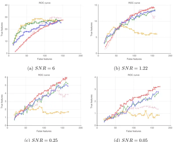
as 𝑛 increases, on regression instances satisfying the mutual incoherence condition, with fixed support size . . . 62 2-4 Number of true features 𝑇 𝐹 vs. number of false features 𝐹 𝐹 of

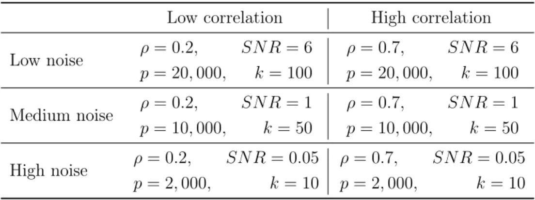
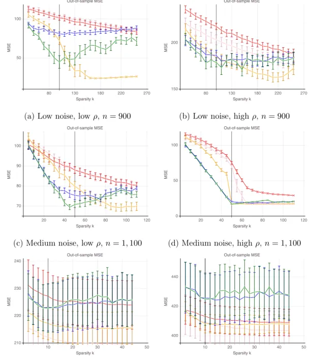
differ-ent feature selection methods as 𝑘 increases, on regression instances satisfying the mutual incoherence condition . . . 64 2-5 Out-of-sample mean square error of different feature selection methods

as 𝑘 increases, on regression instances satisfying the mutual incoherence condition . . . 65 2-6 Accuracy of different feature selection methods as 𝑛 increases, on

regression instances satisfying the mutual incoherence condition, with cross-validated support size . . . 66 2-7 False detection rate of different feature selection methods as 𝑛 increases,

on regression instances satisfying the mutual incoherence condition, with cross-validated support size . . . 67

2-8 Accuracy and out-of-sample mean square error of different feature selection methods as 𝑛 increases, on regression instances violating the mutual incoherence condition, with fixed support size . . . 69 2-9 Accuracy and false detection rate of different feature selection methods

as 𝑆𝑁𝑅 increases, on regression instances constructed from a real-world design matrix 𝑋 . . . 71 2-10 Number of true features 𝑇 𝐹 vs. false features 𝐹 𝐹 of different feature

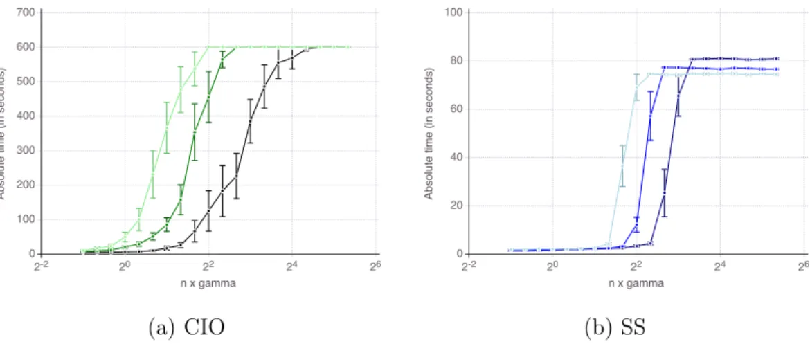
selection methods as 𝑘 increases, on regression instances from a real-world design matrix 𝑋 and for varying noise regimes . . . 72 2-11 Computational time of the cutting plane and the sub-gradient

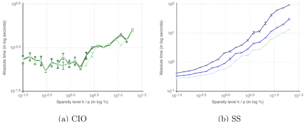
algo-rithms as the regularization parameter 𝑛 × 𝛾 increases . . . 77 2-12 Computational time of the cutting plane and the sub-gradient

algo-rithms as the sparsity parameter 𝑘 increases . . . 78 2-13 Computational time of different feature selection methods as the

signal-to-noise ration 𝑆𝑁𝑅 or the correlation 𝜌 increase . . . 78 2-14 Computational time of different feature selection methods as 𝑛 and 𝑝

increase, on regression instances . . . 79 2-15 Out-of-sample mean square error of different feature selection methods

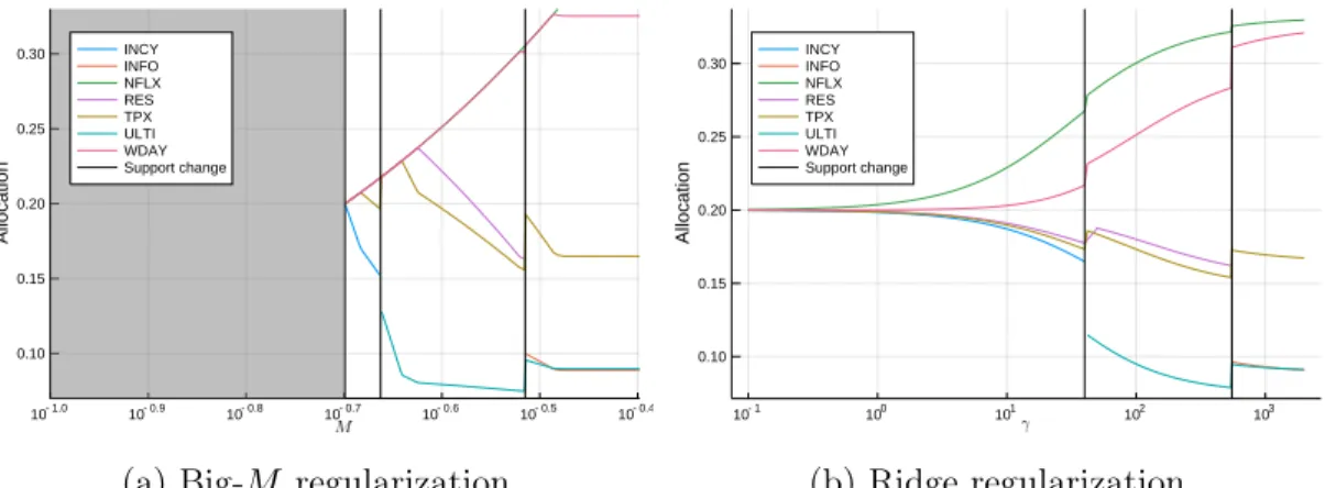
as signal-to-noise 𝑆𝑁𝑅 increases, on regression instances constructed from a real world design matrix 𝑋 . . . 79 3-1 Optimal allocation of funds between securities as the regularization

parameter (𝑀 or 𝛾) increases . . . 115 3-2 Magnitude of the normalized absolute bound gap as the regularization

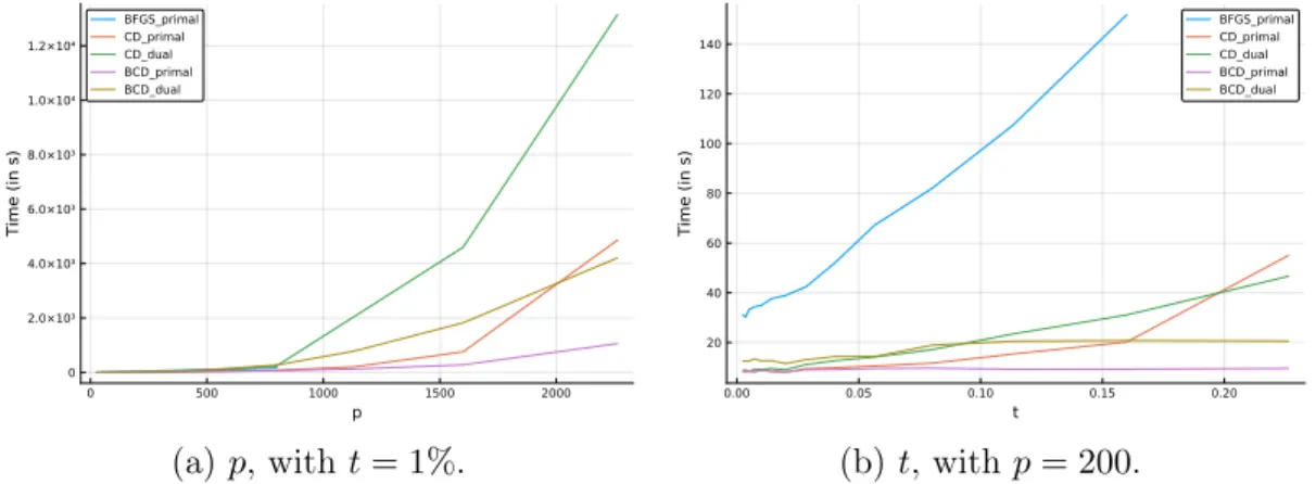
parameter (𝑀 or 𝛾) increases, for the portfolio selection problem studied in Figure 3-1 . . . 115 4-1 Impact of dimension size 𝑝 and sparsity level 𝑡 on computational time,

for the big-𝑀 regularization with 𝑀 = 𝑀0 = 𝑝/‖Σ‖1 . . . 140

4-2 Impact of dimension size 𝑝 and sparsity level 𝑡 on computational time, for the ridge regularization with 𝛾 = 𝛾0 = 4𝑝/‖Σ‖22 . . . 140

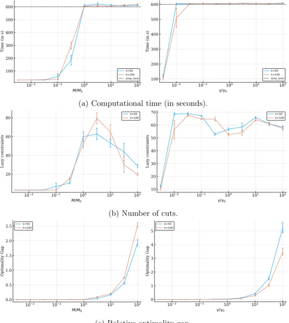
4-3 Impact of the regularization parameter on computational time, number of cuts, and relative optimality gap . . . 143 4-4 Impact of the number of samples 𝑛/𝑝 on support recovery, when the

hyper-parameters are chosen using negative log-likelihood . . . 145 4-5 Impact of the sparsity level 𝑡 on support recovery, when the

hyper-parameters are chosen using negative log-likelihood . . . 146 4-6 Impact of the number of samples 𝑛/𝑝 on out-of-sample negative

log-likelihood . . . 155 4-7 Impact of the number of samples 𝑛/𝑝 on support recovery, when the

hyper-parameters are chosen using the 𝐵𝐼𝐶1/2 criterion . . . 155

4-8 Impact of the sparsity level 𝑡 on out-of-sample negative log-likelihood 155 4-9 Impact of the sparsity level 𝑡 on support recovery, when hyper-parameters

are chosen using the 𝐵𝐼𝐶1/2 criterion . . . 156

4-10 Impact of the dimension 𝑝 on support recovery, when the hyper-parameters are chosen using negative log-likelihood . . . 156 4-11 Impact of the dimension 𝑝 on support recovery, when hyper-parameters

are chosen using the 𝐵𝐼𝐶1/2 criterion . . . 157

4-12 Impact of the dimension 𝑝 on out-of-sample negative log-likelihood . . 157 4-13 Impact of the dimension 𝑝 on computational time . . . 157 5-1 Decision tree predicting inpatient mortality . . . 172 5-2 Look-up at a decision tree for predicting whether a patient will stay

more than 7 days on overall . . . 173 5-3 Screenshot of the capacity prediction tool built for the office of bed

management . . . 175 5-4 Comparison of actual and predicted discharge volume between mid-May

2018 and mid-July 2018 . . . 176 5-5 Running average (7-day window) of the absolute error in discharge

5-6 Running average (7-day window) of the absolute error in discharge prediction over a year . . . 180 6-1 Schematic views of patient flows in a typical hospital . . . 198 6-2 Violin plots of the distribution of three waiting time-related metrics

under the historical policy vs. and the (H2O) policy . . . 220

6-3 Boxplot for the distribution of the relative difference between the (H2O)

policy over the historical bed assignment decisions in terms of four performance metrics . . . 221

List of Tables

2.1 Relevant loss functions ℓ and their corresponding Fenchel conjugates ˆℓ 36 2.2 Computational time of the sub-gradient ascent algorithms for data sets

with large values of 𝑛 and 𝑝 . . . 51 2.3 Regimes of noise (𝑆𝑁𝑅) and correlation (𝜌) considered in our

experi-ments on regression with Toeplitz covariance matrix . . . 57 2.4 Regimes of noise (𝑆𝑁𝑅) considered in our regression experiments on

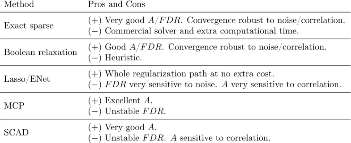
the Cancer data set . . . 70 2.5 Summary of the advantages (+) / disadvantages (-) of each feature

selection method . . . 75 3.1 Summary of the advantages (+) /disadvantages (−) of both

regulariza-tion techniques . . . 99 3.2 Best solution found after one hour on network design instances for

CPLEX vs. cutting plane algorithm and both Big-M and Ridge regu-larization . . . 111 3.3 Average runtime on binary quadratic optimization problems from the

Biq-Mac library Wiegele [2007], Billionnet and Elloumi [2007] . . . . 111 3.4 Average incumbent objective value after 1 hour for medium-scale binary

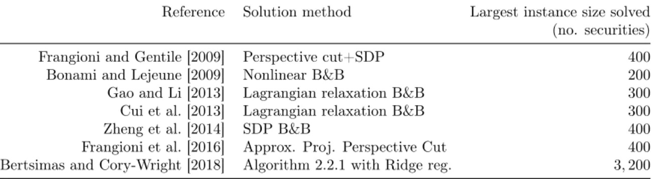
quadratic optimization problems from the Biq-Mac library Wiegele [2007], Billionnet and Elloumi [2007] . . . 112 3.5 Largest sparse portfolio instances reliably solved by each approach . . 113

3.6 Proportion of wins and relative improvement over CPLEX in terms of computational time on the 112 facility location instances from the OR-library [Beasley, 1990, Holmberg et al., 1999] for different imple-mentations of our method . . . 114 3.7 Average runtime per numerical approach, on unit commitment data

from Frangioni and Gentile [2006b] . . . 114 4.1 Average performance on synthetic data where the hyper-parameters are

chosen using the best negative log-likelihood over a validation set . . 144 4.2 Average performance on synthetic data where the hyper-parameters

are chosen using the best in-sample extended Bayesian information criterion 𝐵𝐼𝐶1/2 . . . 144

4.3 Metrics used for prediction performance comparison for the breast cancer dataset . . . 148 4.4 Comparison of estimators on the breast cancer dataset . . . 149 4.5 Average computational performance of the cutting-plane approach on

small-size instances of sparse covariance estimation . . . 154 5.1 Condensed literature review on hospital discharge and length of stay

prediction . . . 161 5.2 Summary statistics of the study population for hospital patient flow

prediction . . . 164 5.3 Summary of the results on predicting hospital length of stay (overall

and remaining) . . . 169 5.4 Summary of the results on predicting discharge destination . . . 170 5.5 Out-of-sample AUC for predicting ICU need . . . 170 5.6 Top 5 variables selected by the random forest classifier for predicting

whether a patient will stay more than 7 days on overall . . . 172 5.7 Predictive error of the machine learning models vs. resource nurses on

hospital discharge volume, during the treated days. Error is measured in terms of relative error compared with actual discharge volume . . . 177

5.8 Difference-in-differences analysis of boarding delays and off-service place-ment, before and after introduction of our machine learning-enhanced dashboard . . . 178 5.9 Comparison of out-of-sample performance for predicting length of stay

(overall and remaining) . . . 186 5.10 Comparison of out-of-sample performance for predicting discharge

des-tination . . . 187 5.11 Median Absolute Error in the daily number of discharges with various

prediction models and aggregation strategies . . . 189 6.1 Summary of the empirical evidence for the impact of off-service and

off-level placement on resulting length-of-stay, mortality rate, and readmission rate . . . 194 6.2 Description of inpatients units on campus E at our partner hospital . 199 6.3 Out-of-sample performance for all patient-flow prediction tasks, on their

respective test set . . . 209 6.4 Summary statistics of the solve time (in seconds) over 1440 instances

of (H2O) . . . 219

6.5 Summary statistics on the relative difference between the (H2O) policy

over the historical bed assignment decisions in terms of peak census, overall throughput and admission from outside transfer . . . 222 6.6 Comparison of individual bed assignement decisions from the (H2O)

policy with the historical bed placements . . . 223 6.7 Description of inpatients units on campus W at our partner hospital . 224

Chapter 1

Introduction

“When I think of the hospital of the future, I think of a bunch of people sitting in a room full of screens and phones,”

says Toby Cosgrove, CEO of Cleveland Clinic [The Economist, 2017]. All major health-care providers such as the Cleveland Clinic are rethinking the way hospitals work, for the gap between populations’ health needs and the care offered by systems organized around hospitals has grown ever wider. Indeed, in the past half-century the burden of disease in developed countries has shifted from communicable diseases to chronic conditions related to unhealthy lifestyles and longer lifespans.

In the next ten to twenty years, hospitals will certainly operate more and more like air-traffic control centers whose role is to coordinate care across multiple facilities. Consequently, the future of hospital operations will have three salient characteristics. First, data. The ability to process, analyze and exploit data effectively will become a vital skill for practitioners in the field. Second, a holistic approach. Orchestrating care requires the concurrent optimization of multiple resources, services, and time scales. Third, real-time decisions, to respond to the increasingly closer monitoring of patients. Actually, with the routinization of cloud storage, the ongoing digital transformation of the economy and the widespread adoption of connected devices, healthcare is one out of many industries where data and analytics will pervade their operations and decision making.

To support this transition and transform our healthcare system towards better outcomes at lower costs, research in operations and analytics should address two concurrent goals: First, develop new methods and algorithms for decision-making in a data rich environment, which answer key concerns from practitioners and regulators, such as reliability, interpretability and fairness. Second, put its models and algorithms to the test of practice, to ensure a path towards implementation and impact. This unique positioning, at the interface of theory and practice, is a vital and exciting characteristic of operations research. Practical applications serve as a compass to guide theoretical development, while rigorous methods and theory should provide a backbone to policymakers.

1.1

Methodological challenges in machine learning

and optimization

From the needs of practitioners in high-stake industries like healthcare, we highlight two broad research questions where algorithmic advances are need: sparsity and interpretability in machine learning; and large-scale discrete optimization.

1.1.1

Sparsity and interpretability in machine learning

We often use models to improve our knowledge of a given phenomenon. While the amount and extensity of the data available have exploded in the past decades, it is fair to admit that humans remain limited in their cognitive ability to understand complex models. As Rutherford D. Roger said “We are drowning in information but starving for knowledge”. Hence, the identification of important variables within large data sets of high dimensionality has become increasingly valuable to practitioners and decision makers. Correspondingly, the notion of sparsity, i.e., the property of a model to involve a limited number of covariates, has become cardinal in high-dimensional statistics. We refer skeptic readers to the first chapter of Hastie et al. [2015], which makes a strong case for sparsity in statistical learning.

The two chief problems in statistics, namely maximum likelihood estimation and empirical risk minimization, can be formulated as optimization problems. Given a set of independent identically distributed observations 𝑥1, . . . , 𝑥𝑛∈ R𝑝, the maximization

likelihood estimation (MLE) tries to find the probability distribution within a family 𝒫 that is most likely to have generated the sample, i.e., solves

max 𝑝∈𝒫 𝑛 ∑︁ 𝑖=1 log 𝑝(𝑥𝑖). (MLE)

If we also observe responses 𝑦1, . . . , 𝑦𝑛∈ R, the empirical risk minimization problem

finds the best predictor of 𝑦 given 𝑥 among a prescribed class of learners ℱ, i.e., solves

min 𝑓 ∈ℱ 𝑛 ∑︁ 𝑖=1 ℓ(𝑦𝑖, 𝑓 (𝑥𝑖)), (ERM)

where ℓ(·, ·) is an appropriate loss function measuring the “risk” of predicting 𝑓(𝑥) for 𝑦. To reduce those optimization problems to a finite-dimensional space, the family of probability distributions 𝒫 or the class of learners ℱ is often a parametric family of the form

𝒫 = {𝑝(·|𝜃) : 𝜃 ∈ 𝒯 } or ℱ = {𝑓 (·|𝜃) : 𝜃 ∈ 𝒯 }, where 𝜃 is a finite-dimensional vector of parameters to calibrate.

In this context, sparsity of the model is associated with the number of non-zero coefficients in the parameter vector 𝜃, also called the 0-pseudo norm of 𝜃 and denoted ‖𝜃‖0 := |{𝑗 : 𝜃𝑗 ̸= 0}|. The 0-pseudo norm is not a norm - it is neither

subadditive nor positively homogeneous - and is not even convex. As a result, sparse maximum likelihood or empirical risk minimization problems with an explicit constraint on ‖𝜃‖0 are NP-hard combinatorial problems [Natarajan, 1995], which have often

been considered as intractable in large dimensions and disregarded by the statistical community.

Consequently, much attention has been directed to convex surrogate estimators which tend to be sparse, while requiring less computational effort. The most common

of such methods is the so-called Lasso proposed by Tibshirani [1996], which replaces the non-convex 0-pseudo norm by the ℓ1-norm. The resulting optimization problem

is often convex and can be solved in high dimensions. Its practical success can be explained by three concurrent ingredients: Efficient numerical algorithms exist [Efron et al., 2004, Friedman et al., 2008, 2010, Beck and Teboulle, 2009], off-the-shelf implementations are publicly available [Friedman et al., 2009] and recovery of the true sparsity is theoretically guaranteed under admittedly strong assumptions on the data [Wainwright, 2009b]. However, recent works [Lam and Fan, 2009, Fan and Song, 2010, Su et al., 2017] have pointed out several key deficiencies of the Lasso regressor in its ability to select the true features without including many irrelevant ones as well. For example, one drawback is that the ℓ1-penalty introduces extra bias when estimating

nonzero entries with large absolute values [Lam and Fan, 2009]. In a parallel direction, theoretical work in statistics [Wainwright, 2009a, Wang et al., 2010, Gamarnik and Zadik, 2017] has identified regimes where Lasso fails to recover the true support even though support recovery is possible from an information theoretic point of view.

Therefore, recent research has focused on replacing the ℓ1 norm in the Lasso

formulation by other sparsity-inducing penalties which are less sensitive to noise or correlation between features. In particular, concave penalties such as smoothly clipped absolute deviation (SCAD) [Fan and Li, 2001] and minimax concave penalty (MCP) [Zhang, 2010] have been proposed. Both SCAD and MCP are folded concave penalties that do not introduce extra bias for estimating nonzero entries with large absolute values. Theoretical properties of these methods are well studied [Rothman et al., 2008, Lam and Fan, 2009]. From a computational point of view, coordinate descent algorithms [Breheny and Huang, 2011] have shown very effective, even though lack of convexity in the objective function cannot provide any certificate of optimality and hindered their wide adoption in practice.

Another line of research in numerical algorithms for solving the cardinality-constrained formulation directly has flourished. Leveraging recent advances in mixed-integer solvers [Bertsimas et al., 2016, Bertsimas and King, 2017], Lagrangian re-laxation [Pilanci et al., 2015], cyclic coordinate descent [Hazimeh and Mazumder,

2018], or cutting-plane methods [Bertsimas and Van Parys, 2017], these works have demonstrated significant improvement over existing Lasso-based heuristics. Convinced that sparsity is an extremely valuable property in high-impact applications where interpretability matters, Chapter 2 and 4 contribute to this line of work by developing novel cutting-plane algorithms for problems arising in machine learning under sparsity, namely (ERM) with linear models and inverse covariance estimation.

1.1.2

Algorithms for large-scale discrete optimization

The combinatorial component of sparse statistical learning problems is widely present in the operations research literature at large. Indeed, start-up costs in machine scheduling problems, financial transaction costs, cardinality constraints and fixed costs in facility location problems, among others, can all be modeled with binary decision variables. In particular, many practically relevant optimization problems - such as portfolio selection, facility location, network design, unit commitment - involve logical relationship between some continuous variables 𝑥 and binary variables 𝑧 of the form “𝑥 = 0 if 𝑧 = 0”.

Since the seminal work of Glover [1975], this relationship is usually enforced through a “big-𝑀” constraint of the form −𝑀𝑧 ≤ 𝑥 ≤ 𝑀𝑧 for a sufficiently large constant 𝑀 > 0. On the computational side, a mixed-integer optimization problem with big-𝑀 constraints admits a bounded relaxation and can therefore be solved via branch-and-bound. Moreover, because the relationship between discrete and continuous variables is enforced via linear constraints, a big-𝑀 reformulation has a theoretically low impact on the ability to solve the continuous relaxation. However, in practice, high values of 𝑀 lead to numerical instability and provide low-quality bounds [see Beaumont, 1990, Section 5]. Glover’s work has been so influential that big-𝑀 constraints are now considered as intrinsic components of the initial problem formulations themselves, to the extent that textbooks in the field introduce facility location, network design or sparse portfolio problems with big-𝑀 constraints by default, although they are actually reformulations of logical constraints.

research and management science problems are increasingly larger in size, driven by the widespread adoption of connected devices and remote monitoring. To cope with large problem sizes, a variety of decomposition strategies have been proposed to break down a large problem into subproblems of reduced size and lower memory footprint. The first such decomposition method is known as Benders decomposition and was proposed for linear optimization problems by Benders [1962]. This outer-approximation method was subsequently generalized to account for non-linear integral variables by Duran and Grossmann [1987], Fletcher and Leyffer [1994]. Though slow in their original implementation, decomposition schemes have proven especially effective when implemented as a branch-and-cut approach [Padberg and Rinaldi, 1991, Stubbs and Mehrotra, 1999], which embeds the cut generation process within a single branch-and-bound tree, rather than building a branch-branch-and-bound tree before generating each cut. We refer to Fischetti et al. [2016, 2017] for recent successful implementations of “modern” decomposition schemes for large-scale facility location problems.

In Chapter 3, we propose a unified framework for mixed-integer optimization to synthesize these two areas of the mixed-integer optimization literature which are often considered in isolation: (𝑎) modeling forcing constraints which encode whether continuous variables are active and can take non-zero values or are inactive and forced to 0, and (𝑏) decomposition algorithms for large mixed-integer optimization problems. Notably, our framework includes big-𝑀 as a special case and propose alternatives to model logical constraints, using a strictly convex regularization term. We argue that selecting a way to reformulate logical constraints constitutes a modeling choice, and connect this choice to the efficiency of the aforementioned decomposition schemes.

1.2

Challenges for analytics in healthcare

To improve the quality of care and alleviate the burden on clinicians and hospital staff, healthcare operations practitioners widely agree on the need to shift from isolated improvement in each individual units to a global coordination scheme across the entire hospital. For instance, Rutherford et al. [2017] identified five guiding principles, among

which the utilization of advanced data analytics to “forecast patient demand patterns, and match capacity and demand”. In essence, they advocate for the development of both predictive and prescriptive analytics to improve hospital operations. However, there are unique challenges associated with healthcare when applying such techniques in practice.

1.2.1

Interpretability in healthcare

In order to “forecast patient demand patterns” [Rutherford et al., 2017], combining patient-level information from Electronic Health Records (EHRs) with sophisticated machine learning techniques can provide welcome visibility on patient flows and inform hospital operations.

Despite the richness and increasing availability of data in healthcare, predictive models are not widely deployed in practice, due to the need to create custom dataset with specific variables for each predictive task. To address this issue, Nguyen et al. [2017], Miotto et al. [2016], Rajkomar et al. [2018] proposed automatized patient representation strategies which analyze EHRs and construct relevant features in an unsupervised way using autoencoder neural networks. Since these approaches do not require an expert to manually define features, they are allegedly more scalable. Surprisingly, however, and to the best of our knowledge, none of these approaches has been integrated within an EHR system of a real-world hospital despite their excellent predictive power on retrospective studies, including the most recent one [Rajkomar et al., 2018].

In our opinion, they undermined a major implementation bottleneck: lack of interpretability. The black-box nature of deep learning models impedes adoption from doctors and caregivers which are not engaged in the modeling process. Automation alone does not guarantee scalable implementation. In our experience, involving stakeholders at each point in the process is instrumental in building trust between clinical and analytical teams, and deploying the predictive models in production. Interpretability is also a useful tool to avoid bias in the predictive models that could lead to unfair treatment allocations [Gianfrancesco et al., 2018]. Finally, legislation, such as

the EU General Data Protection Regulation, advances a “right for an explanation” for people subject to automated data-based decisions. Though its practical implementation remains unclear, interpretability of the underlying predictive model will certainly be a prerequisite for this legal imperative of “explainability”.

We experience and address the practical challenges associated with the design and implementation of machine learning models in healthcare in Chapter 5. We build an end-to-end machine learning pipeline to convert raw clinical data from EHRs into a unique patient representation. We propose a simple expertise-driven patient representation framework to capture the state of each inpatient as she stays in the hospital, which competes with black-box deep learning approaches. Using this rich set of covariates, we predict operationally relevant outcomes using interpretable machine learning techniques, thus providing insights and explanations alongside highly accurate predictions. With practical impact in mind, we fully integrate our models into the EHR system of a large academic hospital and design user-friendly dashboards to support daily decision-making.

1.2.2

A system view of hospital operations

“A system-wide approach to patient flow” as promoted by Rutherford et al. [2017] could certainly improve hospital operations and lead to better health outcomes for the patients at lower operational costs.

Armony et al. [2015] conducted one of the first data-based analysis of patient flows at a hospital level. As they acknowledge, “traditionally, hospital studies have focused on individual units, in isolation from the rest of the hospital; but this approach ignores interactions among units”. They consider a sub-network of units composed of the emergency department (ED) and five inpatient units and compare historical patient flows (arrivals, waiting times, length of stays) with stochastic modeling. Since then, empirical and modeling work has helped understand patient flow, the impact of operational efficiency on quality of care, and the interdependence between units. For instance, delays are a common measure of operational efficiency which is also associated with negative health outcomes [Chan et al., 2017b, Mathews et al., 2018].

Prolonged ED waiting time is usually due to unavailability of beds in inpatient units [Shi et al., 2016], thus inviting a better understanding and modeling of discharge patterns [Shi et al., 2016, Chan et al., 2017a, Dong and Perry, 2018, Dai and Shi, 2019].

However, day-to-day operations remain largely designed and optimized at a unit-level, and implementing hospital-wide strategies is easier said than done. In the literature, adequate staffing levels [Green et al., 2006, Yankovic and Green, 2011], refined ward dimensioning [de Bruin et al., 2010, Boulton et al., 2016], optimized triage processes [Saghafian et al., 2012, 2014, Huang et al., 2015], speed-up procedures in the ED Chan et al. [2014] have been proposed for specific units, in isolation from the rest of the hospital. Recent work [Kilinc et al., 2017, Dai and Shi, 2017] investigates how to optimally decide on admission of ED patients into the inpatient units using a queueing framework. However, their approach can only account for a fraction of the hospital and does not scale to the sizes of real-world medical institutions.

In Chapter 6, we achieve hospital-wide patient flow optimization through advanced large-scale discrete optimization techniques. We formulate a unique optimization problem to optimize bed assignment decisions simultaneously for all inpatient units at a large academic hospital. We not only account for admission of ED patients to inpatient beds but also for outside transfers, surgical patients boarding from the post-anesthesia care units, and patient flows within inpatient units.

1.3

Outline and main contributions

This thesis is comprised of two parts, which serve complementary but distinct objectives. Chapter 2, 3 and 4 present methodological contributions to the discrete optimization literature, with particular emphasis on problems emerging from machine learning under sparsity. Chapter 5 and 6 present applications and implementation of machine learning and discrete optimization methods to improve operations at a large academic hospital in Boston.

constraint, which encompasses linear regression, logistic regression and support vector machines as special cases. Sparsity is the property of a statistical model to incorporate only a limited number of explanatory variables and is especially relevant in contexts where interpretability of the model matters at least as much as its accuracy. We propose a combination of a first-order heuristic and a cutting-plane algorithm to successfully compute high-quality solutions for problems with up to 100,000s covariates. On extensive numerical experiments, we demonstrate that our approach provides better feature selection than competitors, with comparable predictive power.

Chapter 3 We generalize this approach to a family of classical mixed-integer optimiza-tion problems, including network design, facility locaoptimiza-tion, unit commitment, sparse portfolio optimization, binary quadratic optimization and sparse learning problems. These problems exhibit logical relationships between continuous and discrete variables, which are usually reformulated linearly using a big-𝑀 formulation. In this chapter, we propose a paradigm shift and express the logical constraints in a non-linear way. By imposing a regularization condition, we reformulate these problems as convex binary optimization problems, which are solvable using an outer-approximation procedure. Under this lens, the big-𝑀 approach becomes a special case of our regularization condition, rather than an ad-hoc modeling convention. In numerical experiments, we establish that a general-purpose numerical strategy, which combines cutting-plane, first-order and local search methods, solves these problems faster and at a larger scale than state-of-the-art mixed-integer linear or second-order cone methods. Among others, we successfully solve network design problems with 100s of nodes and provide solutions up to 40% better than the state-of-the-art.

Chapter 4 We further extend the approach to mixed-integer semidefinite optimization problems, which are notoriously more challenging from a computational aspect. In particular, we consider the statistical problem of maximum likelihood es-timation of sparse inverse covariance matrices and provide the first provably

exact algorithm for solving it. Our cutting-plane approach has the additional benefit of treating separately the combinatorial aspect of the problem from the semi-definite component of it. The method provides provably optimal solutions, and delivers near optimal solutions in minutes for 𝑝 in the 1, 000s and sparsity level of the order of 1%. Computational experiments on both synthetic and real data show that such discrete formulations deliver solutions with increased out-of-sample predictive power and lower false detection rate than existing methods, while being as accurate.

Chapter 5 We consider an exciting application of machine learning methods to predict patient flows within and out of the hospital. We design a general-purpose framework to describe the status of each patient admitted in the hospital, from a clinical as well as social point of view. Based on this unique framework, we train machine learning models to predict seven relevant outcomes with high accuracy, namely length-of-stay, probability of being discharged in the next 24 or 48 hours, discharge destination and the probability of needing an ICU in the next 24 hours. The models are now fully integrated within the Electronic Health Record system of our partner hospital, compute daily predictions for all inpatients with out-of-sample accuracy in the 80%+ range and are daily used by bed management nurses.

Chapter 6 We propose a holistic optimization model to optimize bed assignment at a hospital level. Indeed, poor bed assignment decisions usually result in patients misplacement as well as admission delays, both of which induce negative health outcomes and prolonged length of stay. We formulate an optimization model to allocate patients to beds in the entire hospital, with three salient characteristics: First, we consider the entirety of the hospital and optimize patient flows at a system level. Second, we formulate the problem as a multi-stage robust decision problem so as to inform the first-stage decisions with future bed requests and discharges. Finally, we integrate predictions obtained from the machine learning techniques developed in the previous chapter into the overall flow

optimization problem using a robust optimization approach. We use outputs from machine learning models to build data-driven uncertainty sets for patients’ clinical flows, instead of making stringent distributional assumptions on the arrival and discharge patterns.

1.4

Notations

We use nonbold face characters to denote scalars, lowercase bold faced characters such as 𝑥 to denote vectors, uppercase bold faced characters such as 𝑋 to denote matrices, and calligraphic characters such as 𝒳 to denote sets. We let e (resp. 0) denote the vector of all 1’s (resp. 0’s), with dimension implied by the context. We denote by 𝑒𝑖,

𝑖 = 1, . . . , 𝑝the unit vectors with 1 at the 𝑖th coordinate and zero elsewhere. For 𝑞 > 1, ‖ · ‖𝑞 denotes the ℓ𝑞-norm defined over vectors as ‖𝑥‖𝑞 = (

∑︀

𝑖|𝑥𝑖|𝑞)1/𝑞.

By convention, ‖𝑥‖∞ = max𝑖|𝑥𝑖|. We denote by ⟨·, ·⟩ the Euclidean inner product

and ·⊤ _{the transpose operator, so that ‖𝑥‖}2

2 = ⟨𝑥, 𝑥⟩ = 𝑥

⊤_{𝑥 for any vector 𝑥. For}

any norm ‖ · ‖, its dual norm is denoted ‖ · ‖⋆ and defined as:

‖𝑦‖⋆ := max

𝑥:‖𝑥‖≤1⟨𝑥, 𝑦⟩.

For instance, the dual of the ℓ𝑞-norm is the ℓ𝑝-norm with 𝑝 such that 1/𝑝 + 1/𝑞 = 1.

In particular, the ℓ2-norm is called self-dual for its dual is the ℓ2-norm itself. Unless

otherwise stated, all norms on matrices are vector norms.

For any 𝑛-dimensional vector 𝑥, we denote with 𝑥[𝑗] the 𝑗th largest component of

𝑥. Hence, we have 𝑥[1] > · · · > 𝑥[𝑛]. The set {1, . . . , 𝑛} is concisely denoted [𝑛].

If 𝑥 is a 𝑛-dimensional vector then Diag(𝑥) denotes the 𝑛 × 𝑛 diagonal matrix whose diagonal entries are given by 𝑥. If 𝑋 is a 𝑛×𝑛 matrix, we adopt the convention that 𝑥𝑖 := 𝑋⊤𝑒𝑖 is the 𝑖th row of 𝑋 while 𝑋𝑗 := 𝑋𝑒𝑗 is its 𝑗th column.

Chapter 2

Sparse regression: a discrete

optimization perspective

2.1

Introduction

The identification of important variables within large data sets of high dimensionality has become increasingly valuable to practitioners and decision makers. Correspond-ingly, the notion of sparsity, i.e., the ability to make predictions based on a limited number of covariates, has become cardinal in statistics. The so-called cardinality-penalized estimators for instance minimize the trade-off between prediction accuracy and number of input variables. Though computationally expensive, they have been considered as a relevant benchmark in high-dimensional statistics. Indeed, these estimators are characterized as the solution of the NP-hard problem

min 𝑤∈R𝑝 𝑛 ∑︁ 𝑖=1 ℓ(𝑦𝑖, 𝑤⊤𝑥𝑖) + 𝜆‖𝑤‖0, (2.1)

where ℓ is an appropriate convex loss function, such as the ones reported in Table 2.1 (p. 36). The covariates are denoted by the matrix 𝑋 ∈ R𝑛×𝑝_{, whose rows are the 𝑥}⊤

𝑖 ’s,

and the response data by 𝑦 = (𝑦1, ..., 𝑦𝑛) ∈ R𝑛. Here, ‖𝑤‖0 := |{𝑗 : 𝑤𝑗 ̸= 0}| denotes

can explicitly constrain the number of features used for prediction and solve min 𝑤∈R𝑝 𝑛 ∑︁ 𝑖=1 ℓ(𝑦𝑖, 𝑤⊤𝑥𝑖) s.t. ‖𝑤‖0 6 𝑘, (2.2)

which is likewise an NP-hard optimization problem [Natarajan, 1995]. For decades, such problems have thus been solved using greedy heuristics, such as step-wise regression, matching pursuits [Mallat and Zhang, 1993], or recursive feature elimination (RFE) [Guyon et al., 2002]. Consequently, much attention has been directed to convex Table 2.1: Relevant loss functions ℓ and their corresponding Fenchel conjugates ˆℓ as defined in Proposition 2.1. The observed data is continuous, 𝑦 ∈ R, for regression and categorical, 𝑦 ∈ {−1, 1}, for classification. By convention, ˆℓ equals +∞ outside of its domain. The binary entropy function is denoted 𝐻(𝑥) := −𝑥 log 𝑥 − (1 − 𝑥) log(1 − 𝑥).

Method Loss ℓ(𝑦, 𝑢) Fenchel conjugate ˆℓ(𝑦, 𝛼) Ordinary Least Square 1

2(𝑦 − 𝑢) 2 1 2𝛼 2_{+ 𝑦𝛼} 1-norm SVR (|𝑦 − 𝑢| − 𝜀)+ 𝑦𝛼 + 𝜀|𝛼|for |𝛼| 6 1 2-norm SVR 1 2(|𝑦 − 𝑢| − 𝜀) 2 + 1 2𝛼 2_{+ 𝑦𝛼 + 𝜀|𝛼|}

Logistic loss log (1 + 𝑒−𝑦𝑢) −𝐻(−𝑦𝛼) for 𝑦𝛼 ∈ [−1, 0] 1-norm SVM - Hinge loss max(0, 1 − 𝑦𝑢) 𝑦𝛼 for 𝑦𝛼 ∈ [−1, 0]

2-norm SVM 1

2max(0, 1 − 𝑦𝑢) 2 1

2𝛼

2_{+ 𝑦𝛼 for 𝑦𝛼 ∈ (−∞, 0]}

surrogate estimators which tend to be sparse, while requiring less computational effort. The Lasso estimator, commonly defined as the solution of

min 𝑤∈R𝑝 𝑛 ∑︁ 𝑖=1 ℓ(𝑦𝑖, 𝑤⊤𝑥𝑖) + 𝜆‖𝑤‖1,

and initially proposed by Tibshirani [1996] is widely known and used. Its practical success can be explained by three concurrent ingredients: Efficient numerical algorithms exist [Efron et al., 2004, Friedman et al., 2010, Beck and Teboulle, 2009], off-the-shelf implementations are publicly available [Friedman et al., 2009] and recovery of the true sparsity is theoretically guaranteed under admittedly strong assumptions on the data [Wainwright, 2009b]. However, recent works [Su et al., 2017, Fan and Song, 2010] have pointed out several key deficiencies of the Lasso regressor in its ability to select the

true features without including many irrelevant ones as well. In a parallel direction, theoretical work in statistics [Wainwright, 2009a, Wang et al., 2010, Gamarnik and Zadik, 2017, Bertsimas et al., 2018a] has identified regimes where Lasso fails to recover the true support even though support recovery is possible from an information theoretic point of view.

Therefore, new research in numerical algorithms for solving the exact formulation (2.2) directly has flourished. Leveraging recent advances in mixed-integer solvers [Bertsimas et al., 2016, Bertsimas and King, 2017], Lagrangian relaxation [Pilanci et al., 2015], cyclic coordinate descent [Hazimeh and Mazumder, 2018], or cutting-plane methods [Bertsimas and Van Parys, 2017], these works have demonstrated significant improvement over existing Lasso-based heuristics. To the best of our knowledge, the exact algorithm proposed by Bertsimas and Van Parys [2017] is the most scalable method providing provably optimal solutions to the optimization problem (2.2), at the expense of potentially significant computational time and the use of a commercial integer optimization solver. Furthermore, their algorithm only applies to ordinary least square regression.

Another line of research has focused on replacing the ℓ1 norm in the Lasso

formula-tion by other sparsity-inducing penalties which are less sensitive to noise or correlaformula-tion between features. In particular, non-convex penalties such as smoothly clipped ab-solute deviation (SCAD) [Fan and Li, 2001] and minimax concave penalty (MCP) [Zhang, 2010] have been proposed. Both SCAD and MCP have the so-called oracle property, meaning that they do not require a priori knowledge of the sparsity pattern to achieve an optimal asymptotic convergence rate, which is theoretically appealing. From a computational point of view, coordinate descent algorithms [Breheny and Huang, 2011] have shown very effective, even though lack of convexity in the objective function hindered their wide adoption in practice.

Convinced that sparsity is an extremely valuable property in high-impact applica-tions where interpretability matters, and conscious that the profusion of research on the matter might have caused confusion and provided little guidance to practitioners, we propose with the present paper a comprehensive treatment of state-of-the-art

methods for feature selection in ordinary least square and logistic regression. Our goal is not to provide a theoretical analysis. On the contrary, we selected and evaluated the methods with an eye towards practicality, taking into account both scalability to large data sets and availability of the implementations. In some cases where open-source implementation was not available, we released code on our website, in an attempt to bridge the gap between theoretical advances and practical adoption. Statistical performance of the methods is assessed in terms of Accuracy (𝐴),

𝐴(𝑤) := |{𝑗 : 𝑤𝑗 ̸= 0, 𝑤𝑡𝑟𝑢𝑒,𝑗 ̸= 0}| |{𝑗 : 𝑤𝑡𝑟𝑢𝑒,𝑗 ̸= 0}|

,

i.e., the proportion of true features which are selected, and False Discovery Rate (𝐹 𝐷𝑅),

𝐹 𝐷𝑅(𝑤) := |{𝑗 : 𝑤𝑗 ̸= 0, 𝑤𝑡𝑟𝑢𝑒,𝑗 = 0}| |{𝑗 : 𝑤𝑗 ̸= 0}|

,

i.e., the proportion of selected features which are not in the true support.

2.1.1

Outline and contribution

Our key contributions can be summarized as follows:

• We provide a unified treatment of state-of-the-art methods for feature selection in statistics. More precisely, we cover the cardinality-constrained formulation (2.2), its Boolean relaxation, the Lasso formulation and its derivatives, and the MCP and SCAD penalty. We did not include step-wise regression methods, for they may require a high number of iterations in high dimension and exist in many variants.

• We formulate the cardinality-constrained formulation (2.2) with general convex loss fuction ℓ as a binary convex optimization problem and propose a tractable outer-approximation algorithm to solve it. Our approach generalizes the one in Bertsimas and Van Parys [2017], who only address the case of ordinary least square regression and make extensive use of the closed-form solution available

in this context. Our framework, however, extends to cases where a closed-form solution is not available and includes, in addition to linear regression, logistic regression and SVM among others. Our cutting-plane algorithm scales to data sets for which 𝑛 and 𝑝 are in the 10, 000s and 100, 000s respectively for regression, and 1, 000s and 10, 000s respectively for classification. Our Julia code is freely available.

• Encouraged by theoretical results obtained for the Boolean relaxation of (2.2) by Pilanci et al. [2015], we propose an efficient sub-gradient algorithm to solve it and provide theoretical rate of convergence of our method. We make our code freely available as a Julia package named SubsetSelection. Our first-order algorithm scales to problems with 𝑛, 𝑝 = 100, 000 or 𝑛 = 10, 000 and 𝑝 = 1, 000, 000within minutes, while providing high-quality estimators.

• We compare the performance of all methods on three metrics of crucial interest in practice: accuracy, false detection rate and computational tractability, and in various regimes of noise and correlation.

• More precisely, under the mutual incoherence condition, all methods exhibit a convergence in accuracy, that is the proportion of correct features selected converges to 1 as the sample size 𝑛 increases, in all regimes of noise and correlation. Yet, on this matter, cardinality-constrained and MCP formulations are the most accurate. As soon as mutual incoherence condition fails to hold, ℓ1-based estimators are inconsistent with 𝐴 < 1, while non-convex penalties

eventually perfectly recover the support.

• In addition, we also observe a convergence in false detection rate, namely the proportion of irrelevant features selected converging to 0 as the sample size 𝑛 increases, for some but not all methods: The convex integer formulation and its Boolean relaxation are the only methods which demonstrate this behavior, in low noise settings and make the fewest false discoveries in other regimes. In our experiments, Lasso-based estimators return at least 80% of non-significant

features. MCP and SCAD have a low but strictly positive false detection rate (around 15 − 30% in our experiments) as 𝑛 increases and in all regimes.

• In terms of computational time, the integer optimization approach is unsurpris-ingly the most expensive option. Nonetheless, the computational cost is only one or two orders of magnitude higher than other alternatives and remains affordable in many real-world problems, even high-dimensional ones. Otherwise, the four remaining codes terminate in time comparable with the glmnet implementation of the Lasso, that is within seconds for 𝑛 = 1, 000 and 𝑝 = 20, 000.

In Section 2.2, we present each method, its formulation, its theoretical underpin-nings and the numerical algorithms proposed to compute it. In each case, we point the reader to appropriate references and open-source implementations. We propose and describe our outer-approximation algorithm scheme for (2.2) and our sub-gradient algorithm for the Boolean relaxation of (2.2) also in Section 2.2. In Section 2.3, we compare the methods on synthetic data sets for linear regression. In particular, we observe and discuss the behavior of each method in terms of accuracy, false detection rate and computational time for three families of design matrices and at least three levels noise. Based on these observations, we formulate guidelines for accurate feature selection in practice.

2.2

Sparse regression formulations

In this section, we introduce the different formulations and algorithms that have been proposed to solve the sparse regression problem. We focus on the cardinality-constrained formulation, its Boolean relaxation, the Lasso and Elastic-Net estimators, the MCP and SCAD penalty. For the cardinality-constrained formulation and its Boolean relaxation, we also propose efficient numerical algorithms to solve them at large scale in minutes.

2.2.1

Integer optimization formulation

As mentioned in introduction, a natural way to compute sparse regressors is to explicitly constrain the number of non-zero coefficients, i.e., solve

min 𝑤∈R𝑝 𝑛 ∑︁ 𝑖=1 ℓ(𝑦𝑖, 𝑤⊤𝑥𝑖) s.t. ‖𝑤‖0 6 𝑘, (2)

where ℓ is an appropriate loss function, appropriate in the sense that ℓ(𝑦, ·) is convex for any 𝑦 . In this paper, we focus on Ordinary Least Square (OLS) and Hinge loss, but our approach applies to all loss functions presented in Table 2.1 on page 36. Unfortunately, such a problem is NP-hard [Natarajan, 1995] and believed to be intractable in practice. The original attempt by Furnival and Wilson [2000] using "Leaps and Bounds" scaled to problems with 𝑛, 𝑝 in the 10𝑠 only. Thanks to both hardware improvement and advances in mixed-integer optimization solvers, Bertsimas et al. [2016], Bertsimas and King [2017] successfully used discrete optimization techniques to solve instances with 𝑛, 𝑝 in the 1, 000s within minutes. In this chapter, we propose a cutting-plane algorithm which extends the results of Bertsimas and Van Parys [2017] to data sets with 𝑛, 𝑝 in the 100, 000s for ordinary least square and 𝑛, 𝑝 in the 10, 000s for logistic regression. To the best of our knowledge, our approach is the only method which scales to instances of such sizes, while provably solving such an NP-hard problem.

Convex integer formulation

As in Bertsimas and Van Parys [2017], we consider an ℓ2-regularized version of the

initial formulation (2.2), min 𝑤∈R𝑝 𝑛 ∑︁ 𝑖=1 ℓ(𝑦𝑖, 𝑤⊤𝑥𝑖) + 1 2𝛾‖𝑤‖ 2 2 s.t. ‖𝑤‖0 6 𝑘, (2.3)

where 𝛾 > 0 is a regularization coefficient. From a statistical point of view, this extra regularization, referred to as ridge or Tikhonov regularization, is needed to account for correlation between features [Hoerl and Kennard, 1970] and mitigate the effect of noise. Indeed, regularization and robustness are two intimately connected properties,

as illustrated by Bertsimas and Copenhaver [2018], Xu et al. [2009b]. In addition, Breiman [1996] proved that subset selection is a very unstable problem and highlighted the stabilizing effect of ridge regularization. Introducing a binary variable 𝑧 ∈ {0, 1}𝑝

to encode the support of 𝑤, problem (2.3) can be formulated as

min 𝑧∈{0,1}𝑝_:𝑧⊤_{𝑒6𝑘 𝑤∈R}min𝑝 𝑛 ∑︁ 𝑖=1 ℓ(𝑦𝑖,Diag(𝑧)𝑤⊤𝑥𝑖) + 1 2𝛾‖Diag(𝑧)𝑤‖ 2 2.

Effectively, the bilinear term Diag(𝑧)𝑤 = (𝑧𝑗𝑤𝑗)𝑗=1,...,𝑝 enforces that a feature 𝑗 does

not contribute to the prediction whenever 𝑧𝑗 = 0. Using convex duality, problem (2.3)

can then be shown equivalent to a convex integer optimization problem as stated in the following theorem.

Proposition 2.1. For any convex loss function ℓ, problem (2.3) is equivalent to min 𝑧∈{0,1}𝑝_:𝑧⊤_{𝑒6𝑘 𝛼∈R}max𝑛 𝑔(𝛼, 𝑧), (2.4) where 𝑔(𝛼, 𝑧) := − 𝑛 ∑︁ 𝑖=1 ˆ ℓ(𝑦𝑖, 𝛼𝑖) − 𝛾 2 𝑝 ∑︁ 𝑗=1 𝑧𝑗𝛼⊤𝑋𝑗𝑋𝑗⊤𝛼,

and ˆℓ(𝑦, 𝛼) := max𝑢∈R{𝑢𝛼 − ℓ(𝑦, 𝑢)} is the Fenchel conjugate of the loss function ℓ

[see Lauritzen, 2013, Chap. 3.3] , as reported in Table 2.1. In particular, the function 𝑔 is continuous, linear in 𝑧 and concave in 𝛼.

The proof of Proposition 2.1 can be found Bertsimas et al. [2018a, Theorem 1]. We omit it in this manuscript for we will prove a more general result in Chapter 3, to which Proposition 2.1 is a special case.

Denoting

𝑓 (𝑧) := max

our goal is then to solve the purely discrete optimization problem

min

𝑧∈{0,1}𝑝 𝑓 (𝑧)s.t. 𝑧

⊤

𝑒 6 𝑘. (2.5)

The above formulation calls for a few observations:

1. 𝑓(𝑧) is a point-wise maximum of linear, hence convex, functions of 𝑧. As a result, 𝑓(·) is a convex function of 𝑧 and the minimization problem above is well defined.

2. Given a feasible support 𝑧 ∈ {0, 1}𝑝_{, we denote by 𝛼}⋆_{(𝑧) the associated dual}

variable, i.e., 𝑓(𝑧) = 𝑔(𝛼⋆_{(𝑧), 𝑧). Then for any feasible 𝑧}′_{, we have}

𝑓 (𝑧′) = max 𝛼∈R𝑛𝑔(𝛼, 𝑧 ′ ) ≥ 𝑔(𝛼⋆(𝑧), 𝑧′) = 𝑓 (𝑧) − 𝛾 2 𝑝 ∑︁ 𝑗=1 (𝑧_𝑗′ − 𝑧𝑗)𝛼⋆(𝑧)⊤𝑋𝑗𝑋𝑗⊤𝛼 ⋆ (𝑧).

The inequality above provides a linear lower-approximation of 𝑓(·) which coin-cides with 𝑓(·) at 𝑧. In particular, it proves that (︀−𝛾

2𝛼

⋆_(𝑧)⊤_𝑋

𝑗𝑋𝑗⊤𝛼⋆(𝑧)

)︀

𝑗=1,...,𝑝

is a subgradient of 𝑓 at 𝑧. This observation plays a central role in devising an efficient numerical strategy to solve this combinatorial problem.

3. In the special case of OLS, the function ℎ is a quadratic function in 𝛼

𝑔(𝛼, 𝑧) = −1 2‖𝛼‖ 2_{− 𝑦}⊤_{𝛼 −}𝛾 2𝛼𝑋𝑧𝑋 ⊤ 𝑧𝛼, where 𝑋𝑧𝑋𝑧⊤ := ∑︀𝑝

𝑗=1𝑧𝑗𝑋𝑗𝑋𝑗⊤. As a result, the inner maximization problem

can be solved in closed form: The maximum is attained at 𝛼⋆_{(𝑧) = −(𝐼} 𝑛+

𝛾𝑋𝑧𝑋𝑧⊤)−1𝑦 and the objective value is

𝑓 (𝑧) = max 𝛼 ℎ(𝛼, 𝑧) = 1 2𝑦 ⊤ (𝐼𝑛+ 𝛾𝑋𝑧𝑋𝑧⊤) −1 𝑦.

4. In the general case, computing 𝑓(𝑧) is equivalent to solving a regularized regression or classification problem to predict 𝑦 given 𝑋𝑧, i.e., using only the

algorithms and off-the-shelf implementation for solving this problem in the case of logistic and Hinge loss, notably coordinate descent algorithms [Hsieh et al., 2008, Yu et al., 2011, Keerthi et al., 2005, see].

Cutting-plane algorithm

For a given support 𝑧, we can evaluate 𝛼⋆_{(𝑧) and compute both the value 𝑓(𝑧) and}

a sub-gradient ∇𝑓(𝑧) of the function by solving a continuous concave maximization problem. Consequently, a valid numerical strategy for minimizing 𝑓(𝑧) comprises of iteratively minimizing a piecewise linear lower-approximation of 𝑓 and refining this approximation at each step until some approximation error 𝜀 is reached, as described in Algorithm 2.2.1. This process is equivalent to constraint generation: Applying the sub-gradient inequality at all feasible supports, 𝑓 can indeed be seen as a piece-wise linear convex function with an exponential number of pieces:

𝑓 (𝑧′) = max{︀𝑓 (𝑧) + ∇𝑓 (𝑧)⊤(𝑧′− 𝑧) : 𝑧 ∈ {0, 1}𝑝, 𝑧⊤𝑒 ≤ 𝑘}︀ , ∀𝑧′,

and the algorithm iteratively includes new pieces. The method has been equivalently referred to in the literature as generalized Benders decomposition. This scheme was independently proposed for continuous decision variables by Cheney and Goldstein [1959] and Kelley [1960], and later extended to binary decision variables by Duran and Grossmann [1987], who provide a proof of termination in a finite, yet exponential in the worst case, number of iterations.

In its naive implementation, the outer-approximation algorithm 2.2.1 solves a large mixed-integer linear optimization problem each iteration. To avoid building a branch and bound tree at each iteration, as suggested in the pseudo-code, this strategy can be integrated within a single branch-and-bound procedure using lazy callbacks. When a constraint is added, instead of resolving the problem, the constraint is added to all active nodes in the current branch-and-bound tree. This enables the same tree to be used for all iterations and provides significant speed-ups for outer-approximation algorithms. Lazy constraint callbacks are now standard tools in commercial solvers.