HAL Id: halshs-02443364
https://halshs.archives-ouvertes.fr/halshs-02443364
Preprint submitted on 17 Jan 2020HAL is a multi-disciplinary open access archive for the deposit and dissemination of sci-entific research documents, whether they are pub-lished or not. The documents may come from teaching and research institutions in France or abroad, or from public or private research centers.
L’archive ouverte pluridisciplinaire HAL, est destinée au dépôt et à la diffusion de documents scientifiques de niveau recherche, publiés ou non, émanant des établissements d’enseignement et de recherche français ou étrangers, des laboratoires publics ou privés.
Extended Markov-Switching Dynamic Factor Model
Catherine Doz, Laurent Ferrara, Pierre-Alain Pionnier
To cite this version:
Catherine Doz, Laurent Ferrara, Pierre-Alain Pionnier. Business cycle dynamics after the Great Recession: An Extended Markov-Switching Dynamic Factor Model. 2020. �halshs-02443364�
WORKING PAPER N° 2020 – 03
Business cycle dynamics after the Great Recession: An Extended
Markov-Switching Dynamic Factor Model
Catherine DOZ
Laurent FERRARA
Pierre-Alain PIONNIER
JEL Codes: C22, C51, E32, E37
Keywords: Markov-Switching Dynamic Factor Model (MS-DFM), Great
Moderation, Great Recession, Turning-Point Detection, Macroeconomic
Forecasting
Business cycle dynamics after the Great Recession:
An Extended Markov-Switching Dynamic Factor Model
Catherine DOZ1
Paris School of Economics (PSE) and University Paris 1 Panthéon-Sorbonne,
Laurent FERRARA
SKEMA Business School – University Côte d’Azur
Pierre-Alain PIONNIER OECD, Statistics and Data Directorate
1 We would like to thank Marcelle Chauvet, Guillaume Chevillon, Arnaud Dufays, Domenico Giannone, Sylvia Kaufmann, Siem-Jan Koopman, Josefine Quast, Luca Sala, Paul Schreyer, Dave Turner, and participants at the 2018 OxMetrics User Conference, the 2018 French Econometrics Conference, the 2019 Symposium of the Society for Nonlinear Dynamics and Econometrics (SNDE), the 2019 Conference of the International Association for Applied Econometrics (IAAE), the 2019 (3rd) Conference on Forecasting at Central Banks, the 2019 Conference on Real-Time Data Analysis, Methods and Applications, the 2019 CIRET/KOF/OECD/INSEE Workshop, and OECD, Namur University and Bocconi University seminars for helpful comments and suggestions.
Abstract: The Great Recession and the subsequent period of subdued GDP growth in most advanced economies have highlighted the need for macroeconomic forecasters to account for sudden and deep recessions, periods of higher macroeconomic volatility, and fluctuations in trend GDP growth. In this paper, we put forward an extension of the standard Markov-Switching Dynamic Factor Model (MS-DFM) by incorporating two new features: switches in volatility and time-variation in trend GDP growth. First, we show that volatility switches largely improve the detection of business cycle turning points in the low-volatility environment prevailing since the mid-1980s. It is an important result for the detection of future recessions since, according to our model, the US economy is now back to a low-volatility environment after an interruption during the Great Recession. Second, our model also captures a continuous decline in the US trend GDP growth that started a few years before the Great Recession and continued thereafter. These two extensions of the standard MS-DFM framework are supported by information criteria, marginal likelihood comparisons and improved real-time GDP forecasting performance.
Keywords: Markov-Switching Dynamic Factor Model (MS-DFM), Great Moderation, Great Recession, Turning-Point Detection, Macroeconomic Forecasting
1. Introduction
Even though GDP is now widely recognised as an insufficient indicator to fully assess the health of an economy and how people are benefitting from economic growth (Stiglitz et al. 2018), it is also clear that recessions measured by GDP and other traditional macroeconomic indicators can have deep and long-lasting effects on people’s (economic) well-being. For example, it is only at the end of 2017, nearly 10 years after the Great Recession of 2008-09, that the average unemployment rate in OECD countries fell back to its pre-crisis level. Moreover, the decline in subjective well-being has been especially visible in OECD countries most affected by the crisis (OECD 2013). Therefore, being able to detect recessions using the macroeconomic information that is available in real time, thus allowing to take adequate policy measures, is of key interest to policy makers. The Great Recession, as well as the years following it, have been difficult times for macroeconomic forecasters. After making large forecast errors at the time of the Great Recession (Lewis and Pain 2015, An et al. 2018), the vast majority of macroeconomic forecasters have tended to systematically over-estimate GDP growth from 2011 to 2017, mainly by assuming long-term mean reversion in their forecasts, i.e. that economic growth would rapidly revert back to its long-term average (see Ferrara and Marsilli 2017 for an assessment of IMF forecasts). In addition, changes in macroeconomic volatility over the last decade further complicated the task of forecasters: after two decades of dampened macroeconomic fluctuations, referred to as the “Great Moderation” period (McConnell and Perez-Quiros, 2000), macroeconomic volatility increased during the Great Recession and apparently subsequently went down (Charles et al. 2018, Gadea-Rivas et al., 2018).
In this paper, we consider small-scale Markov-Switching Dynamic Factor Models (MS-DFMs) as our starting point. These models, whose dynamics depends on whether the economy is in expansion or recession, are increasingly used for short-term forecasting and turning point detection (Chauvet and Potter 2013, Camacho et al. 2014, 2018). They have been introduced by Diebold and Rudebusch (1996) to simultaneously account for co-movement in macroeconomic time series and different dynamics during expansion and recession phases, two business cycle facts that were originally identified by Burns and Mitchell (1946). Chauvet and Piger (2008) and Hamilton (2011) later confirmed the very good empirical performance of small-scale MS-DFMs to track US recessions. They showed that MS-DFMs using the four monthly series advocated by the NBER Business Cycle Dating Committee (industrial production, real manufacturing trade and sales, real personal income excluding transfer payments and non-farm payroll employment) as observable variables are able to accurately replicate the NBER dating of US recessions in a fully transparent way. In addition, they showed that such models are able to identify business cycle phases faster than the NBER, especially around troughs. According to them, those small-scale MS-DFMs also compare favourably to the univariate Markov-Switching model of Hamilton (1989), which only extracts information from the US quarterly GDP series, and to the non-parametric multivariate algorithm of Harding and Pagan (2006), when it is used to extract information from the four monthly series advocated by the NBER for the dating of business cycles.
Against this background, our contribution to the literature is to put forward an Extended MS-DFM which is able to replicate the two recent empirical stylised facts observed since the Great Recession. The first one is the period of subdued GDP growth observed in most advanced economies since the Great Recession, or even slightly before. Deciding whether advanced economies have entered a period of secular stagnation and identifying causes for this stagnation is naturally of key interest for long-term forecasters and policy makers.
Nevertheless, Antolin-Diaz et al. (2017) also argue that, given the fact that standard DFM forecasts revert very quickly to the unconditional mean of GDP, accounting for a possible decline in long-term GDP growth may improve GDP forecasts even at very short horizons. Thus, we propose to integrate a time-varying GDP trend into a small-scale MS-DFM. As shown by Antolin-Diaz et al. (2017), the explicit modelling of time variation in long-run GDP growth is likely to deliver substantial gains in out-of-sample forecasting performance for the US after the Great Recession. To account for the second stylized fact (i.e. changing macroeconomic volatility), we allow for switches in volatility in the state equation of the model, according to a Markov chain that differs from the one we use for the conditional mean. Our approach can be linked to that of Chauvet and Su (2014) who put forward a univariate model with changes in mean and volatility governed by Markov-Switching processes, as well as structural breaks.
Based on US data, we show that the introduction of Markov-Switching volatility in the standard MS-DFM framework is supported by statistical criteria (DICs and marginal likelihoods) and improves the detection of turning points after the mid-1980s. The Extended MS-DFM also accurately detects the Great Recession in advance to NBER announcements. The timely detection that the economy has switched to a recession regime allows an improvement of real-time GDP forecasts during the Great Recession as compared to those stemming from a linear DFM incorporating the same amount of information. The introduction of a time-varying long-term GDP growth rate is most helpful to improve real-time GDP forecasts after the Great Recession.
As a by-product of the estimation of our Extended MS-DFM on US data, we also get two interesting results. First, we note a decline in the US long-run GDP growth rate of about one p.p. per year as compared to the early 2000s, half of it occurring before the Great Recession. Such decline in long-run US GDP growth has been empirically documented by Antolin-Diaz et al. (2017) and rationalised by Fernald et al. (2017) who highlight the role of total factor productivity and labour force participation. Second, we conclude that the Great Recession did not put an end to the Great Moderation. According to our model, the Great Recession, beyond its effect on GDP growth, was characterised by a temporary increase in macroeconomic volatility in 2008-09, but we observe a return to a low-volatility environment from 2010 onwards. This result is important for the calibration of macroeconomic models and for the forecasting of future US recessions. It is also in line with recent economic research (Charles et al., 2018, Gadea-Rivas et al., 2018).
The present paper is organised as follows. In Section 2, we review the related literature. In Section 3, we extend the standard MS-DFM framework to account for both switches in macroeconomic volatility and time variation in long-term GDP growth. In Section 4, we describe a Bayesian (Gibbs-sampling) methodology to estimate this model. In Section 5, we provide in-sample estimation results based on US data from 1970 to 2017. In Section 6, we evaluate the real-time out-of-sample properties of our model.
2. Related literature
Initially introduced in the literature by Diebold and Rudebusch (1996), Markov-Switching Dynamic Factor Models (MS-DFMs) have two attractive features: they allow to simultaneously account for co-movement in macroeconomic time series, and for different dynamics during expansion and recession phases. Chauvet (1998) and Kim and Nelson (1998) later proposed maximum likelihood and Bayesian estimation strategies for these models.
In this paper, we put forward an Extended MS-DFM that also incorporates a time-varying long-run GDP growth and Markov-Switching volatility. Our model can be seen as a non-linear extension of the model proposed by Antolin-Diaz et al. (2017), who include a time-varying long-run GDP growth rate in an otherwise linear DFM model. Our main difference with them is the inclusion of Markov-Switching features in the state equation of our model to disentangle expansion from recession phases, as well as high-volatility from low-volatility regimes.
Like Antolin-Diaz et al. (2017) and Marcellino et al. (2016), we account for time-variation in macroeconomic volatility, but whereas they rely on a stochastic volatility specification, we rely on a Markov-Switching volatility specification. The evidence provided by Sensier and van Dijk (2004) supports this specification. Indeed, they document that the vast majority (80%) of US macroeconomic variables experienced a reduction in (conditional) volatility after 1980 and that these volatility changes are better characterised by instantaneous breaks than by gradual changes. Stock and Watson (2002) also conclude that the Great Moderation episode is better accounted for by a sharp break in volatility rather than a gradual decline, thus reflecting a reduction in the size of shocks hitting the economy more than a change in the propagation mechanism of these shocks. Our model is closely connected to the one proposed by Eo and Kim (2016) who relax the assumption that all recessions and expansions are alike in a univariate Markov-Switching model of the business cycle. But whereas Eo and Kim (2016) allow for a fully flexible evolution of the regime-specific mean growth rates over time, with random walks on the long-run GDP growth rate and the regime-specific mean growth rates, we relate evolutions in regime-specific mean growth rates to evolutions in macroeconomic volatility, as proposed by McConnell and Perez-Quiros (2000), Giordani et al. (2007) and Bai and Wang (2011). It is also connected to the model proposed by Chauvet and Su (2014), who include independent Markov-Switching processes for the mean and the variance of GDP growth, and add a structural break in GDP growth, whereas we put forward a time-varying long-run GDP growth rate.
In this paper, we consider a larger information set than Eo and Kim (2016) or Chauvet and Su (2014), and include the four monthly variables advocated by the NBER in addition to quarterly GDP, the only variable that they consider. The fact that we consider a multivariate framework also distinguishes the present model from the univariate models of McConnell and Perez-Quiros (2000), Giordani et al. (2007) and Bai and Wang (2011). In addition, extracting a common factor from multiple series also makes it less important to explicitly account for outliers in individual observed series, as advocated by Giordani et al. (2007). Note that our information set could easily be expanded to include additional monthly or quarterly indicators, which makes our model suitable for nowcasting GDP growth.
Similarly to us, Eo and Morley (2017) also consider two types of recessions and allow for a break in trend GDP growth in 2006Q1. Nevertheless, they do not relate the two recession types to macroeconomic volatility but distinguish L-shaped recessions, with a permanent effect on the level of GDP, and U-shaped recessions, with only a transitory
effect on the level of GDP. Like Eo and Kim (2016), their information set only includes US quarterly GDP. Based on this specification, they conclude that the Great Recession was U-shaped and that the US economy fully recovered from it in 2014.
Antolin-Diaz et al. (2017), Eo and Kim (2016) and Eo and Morley (2017) identify a decrease in US trend GDP growth which started before the Great Recession, but its precise timing and magnitude differ. Antolin-Diaz et al. (2017) conclude that the US long-run GDP growth has declined from a peak of 3.5% per year around 2000 to about 2.0% per year in 2015. Eo and Kim (2016) identify a continuous decrease in US trend GDP growth from 3.6% per year in the 1950s to 2.0% per year around 2010, with no noticeable peak around 2000. 2 Finally, Eo and Morley (2017) report a break of -0.52% per quarter (or - 2.06% per year) in US trend GDP growth in 2006Q1. The differences between these three estimates may be related to differences in information sets (16 monthly and quarterly series for Antolin-Diaz et al. (2017), US quarterly GDP growth for both Eo and Kim (2016) and Eo and Morley (2017)), differences in the modelling of trend GDP growth (continuous variation for both Antolin-Diaz et al. (2016) and Eo and Kim (2016), discrete break for Eo and Morley (2017)), and differences in the modelling of cyclical fluctuations.
Table 1 summarises how the present paper relates to the existing literature.
Table 1. Comparison with the existing literature
Multivariate framework (factor model) Markov-Switching Intercept Markov-Switching volatility of shocks Stochastic volatility Time-varying long-term GDP growth rate Antolin-Diaz et al. (2017) X X X
Bai and Wang
(2011) X X Chauvet and Su (2014) X X Diebold and Rudebusch (1996) X X Eo and Kim (2016) X X X Giordani et al. (2007)3 X X X
Kim and Nelson
(1998) X X Marcellino et al. (2016) X X McConnell and Perez-Quiros (2000) X X This paper X X X X 2
Eo and Kim (2016) actually report quarterly figures. 3
Giordani et al. (2007) actually consider the dynamics of industrial production (IP) in G7 countries. Thus, they introduce time variation in the long-term growth rate of IP, not GDP, but do it in a very similar way as in the present paper and Antolin-Diaz et
3. Specification of the Extended MS-DFM
The factor model with Markov-Switching mean was introduced by Diebold and Rudebusch (1996) and estimated in a Bayesian way (Gibbs Sampling) by Kim and Nelson (1998). In the model we put forward in this paper, it is assumed that both the intercept and the volatility of shocks in the state equation (factor dynamics) are governed by two independent Markov-Switching processes. This specification can be thought as a generalisation of McConnell and Perez-Quiros (2000) to a multivariate framework. Indeed, McConnell and Perez-Quiros (2000) only considered US quarterly GDP as observable variable, whereas we consider the four monthly series explicitely mentioned by the business cycle Dating Committee of the NBER, in addition to quarterly GDP. Let us first consider a general state-space model where, for the time being, all the n observable variables yit are available at monthly frequency. This model is given by the
two following equations:
Measurement equations (for i = 1,...,n): ∆𝑦𝑖𝑡 = 𝑎𝑖,𝑡+ 𝛾𝑖(𝐿)∆𝑐𝑡+ 𝑢𝑖𝑡
State equations: { 𝑎𝑖,𝑡= 𝑎𝑖,𝑡−1+ 𝜎𝑎,𝑖∙ 𝜂𝑡𝑎,𝑖 ; 𝜂𝑡𝑎,𝑖~𝐼𝐼𝐷 𝑁(0,1) 𝜙(𝐿)∆𝑐𝑡= 𝜇𝑆𝑡,𝑉𝑡+ √1 + ℎ ∙ 𝑉𝑡∙ 𝜎𝑐∙ 𝜂𝑡 𝑐 ⏟ 𝑉𝑎𝑟𝑖𝑎𝑛𝑐𝑒 = 𝜎𝑐2 𝑖𝑛 𝑡ℎ𝑒 𝑙𝑜𝑤−𝑣𝑜𝑙𝑎𝑡𝑖𝑙𝑖𝑡𝑦 𝑟𝑒𝑔𝑖𝑚𝑒, 𝑎𝑛𝑑 (1+ℎ)∙ 𝜎𝑐2 𝑖𝑛 𝑡ℎ𝑒 ℎ𝑖𝑔ℎ−𝑣𝑜𝑙𝑎𝑡𝑖𝑙𝑖𝑡𝑦 𝑟𝑒𝑔𝑖𝑚𝑒 ; 𝜂𝑡𝑐~𝐼𝐼𝐷 𝑁(0,1) 𝜓𝑖(𝐿)𝑢𝑖𝑡 = 𝜎𝑖∙ 𝜀𝑖𝑡 ; 𝜀𝑖𝑡~𝐼𝐼𝐷 𝑁(0,1)
In the measurement equations, the ∆𝑐𝑡 component captures common fluctuations across
observable variables and the 𝑎𝑖,𝑡 variables capture potential low-frequency variations in
mean growth rates, such as the slow decline in the GDP growth rate, as in Giordani et al. (2007) and Antolin-Diaz et al. (2017). This random walk that we introduce in the data generating process of the GDP growth rate should only be considered as a convenient modelling simplification. It allows to capture the low-frequency component of the time series and remains innocuous over a limited period of time. Our approach can also be related to the one of Stock and Watson (2012) who subtract a local mean to the US GDP growth rate before including it in their model. In our case, this adjustment is made within the model.
In the state equations, the 𝑎𝑖,𝑡 variables are modelled as independent random walks, the
common component ∆𝑐𝑡 follows an autoregressive process with Markov-Switching
intercept and Markov-Switching variance, and the error terms 𝑢𝑖𝑡 are modelled as
independent autoregressive processes. Thus, we allow the error terms of the measurement equations to be autocorrelated, but not cross-correlated. The fact that the business cycle, proxied by the common factor, directly depends on the volatility is based on the literature pointing out that second moments are useful to predict macroeconomic fluctuations (see McConnell and Perez-Quiros 2000, Bai and Wang 2011, and Chauvet et al. 2015). In addition, 𝑆𝑡 and 𝑉𝑡 are two independent first-order Markov-Switching processes, each
with only two possible states (0 and 1). Transition probabilities are given by: 𝑝(𝑆𝑡 = 0|𝑆𝑡−1= 0) ≡ 𝑃𝑟𝑆00 ; 𝑝(𝑆𝑡= 1|𝑆𝑡−1= 1) ≡ 𝑃𝑟𝑆11
And the intercept of the state equation is such that: 𝜇𝑆𝑡,𝑉𝑡 ≡ 𝜇00+ 𝜇⏟01 <0 ∙ 𝑉𝑡+ 𝜇⏟10 >0 ∙ 𝑆𝑡+ 𝜇⏟11 >0 ∙ 𝑆𝑡∙ 𝑉𝑡 where
𝜇00: Intercept in the low-volatility recession regime
𝜇00+ 𝜇⏟01 <0
: Intercept in the high-volatility recession regime
𝜇00+ 𝜇⏟10 >0
: Intercept in the low-volatility expansion regime
𝜇00+ 𝜇⏟01 <0 + 𝜇⏟10 >0 + 𝜇⏟11 >0
: Intercept in the high-volatility expansion regime
In the empirical part of this paper, we will use a mix of quarterly and monthly data in the information set: the quarterly GDP growth rate and monthly growth rates of industrial production, real manufacturing trade and sales, real personal income excluding transfer payments, and non-agricultural civilian employment. Let us first clarify how the model can accommodate this mix of monthly and quarterly observable variables. Quarterly GDP ∆𝑦1𝑡𝑞 is observed once every three months whereas monthly variables ∆𝑦𝑗𝑡𝑚 are observed every month. This is something that the Kalman filter can easily accommodate. The key to relate quarterly GDP to the underlying monthly state variables is to approximate the quarterly GDP growth rate as a weighted average of current and past monthly GDP growth rates, a solution that has been popularised by Mariano and Murasawa (2003). The five measurement equations can thus be rewritten as follows:
{ ∆𝑦1𝑡 𝑞 = (1 3𝑎1,𝑡 𝑞 +2 3𝑎1,𝑡−1 𝑞 + 𝑎1,𝑡−2𝑞 +2 3𝑎1,𝑡−3 𝑞 +1 3𝑎1,𝑡−4 𝑞 ) + 𝛾1𝑞(𝐿) (1 3∆𝑐𝑡+ 2 3∆𝑐𝑡−1+ ∆𝑐𝑡−2+ 2 3∆𝑐𝑡−3+ 1 3∆𝑐𝑡−4) + (1 3𝑢1,𝑡 𝑞 +2 3𝑢1,𝑡−1 𝑞 + 𝑢1,𝑡−2𝑞 +2 3𝑢1,𝑡−3 𝑞 +1 3𝑢1,𝑡−4 𝑞 ) ∆𝑦𝑗𝑡𝑚= 𝑎𝑗,𝑡𝑚+ 𝛾𝑗𝑚(𝐿)∆𝑐𝑡+ 𝑢𝑗,𝑡𝑚
Then, we assume that quarterly GDP and the first three monthly variables (industrial production, real manufacturing trade and sales, and real personal income excluding transfer payments) are only linked contemporaneously to the business cycle (i.e. to the underlying factor). In other words, we assume that:
𝛾1𝑞(𝐿) = 𝛾10𝑞
𝛾𝑗𝑚(𝐿) = 𝛾𝑗0𝑚 for 𝑗 = 1 … 3
Besides, as in any factor model, we have to impose an identifying restriction (otherwise, the factor would be defined up to a multiplicative constant). Here, we impose the following restriction:
𝛾10 𝑞
For the fourth monthly variable (non-agricultural civilian employment), we include a richer lag structure in order to take into account that employment may be lagging, as in Stock and Watson (1989):
𝛾4𝑚(𝐿) = 𝛾40𝑚+ 𝛾41𝑚𝐿 + 𝛾42𝑚𝐿2+ 𝛾43𝑚𝐿3
Next, we follow Chauvet and Hamilton (2005) in specifying an AR(1) dynamics for the idiosyncratic shocks and the underlying factor, that is:
𝜓1𝑞(𝐿) = 1 − 𝜓11𝑞 𝐿 𝜓𝑗𝑚(𝐿) = 1 − 𝜓𝑗1𝑚𝐿 for 𝑗 = 1 … 4
𝜙(𝐿) = 1 − 𝜙1𝐿
Lastly, we assume that, in our information set, only GDP growth exhibits low-frequency fluctuations, captured by 𝑎1,𝑡𝑞 , which is modelled as a random walk without drift. Since all observable variables are demeaned prior to model estimation, there is no need to add constant terms in the measurement equations. All monthly variables, expressed as monthly growth rates, are assumed to be driven by cyclical fluctuations captured by the underlying factor ∆𝑐𝑡 and the idiosyncratic shocks 𝑢𝑗,𝑡𝑚. This implies 𝑎𝑗,𝑡𝑚 = 0 for 𝑗 =
1 … 4. We thus limit the parameterisation of our model and only explicitly account for low-frequency fluctuations of our main variable of interest, which is GDP growth. Antolin-Diaz et al. (2017) follow a similar modelling strategy and run simulation experiments showing that not including a time-varying trend for the other variables is innocuous for the estimation of the GDP trend as long as persistence is allowed for in the idiosyncratic components of all variables. This is precisely the role of the 𝜓𝑗𝑚(𝐿) polynomials in our model, for which we do not rule out the possibility of having unit roots.
Additional details on the state-space representation of the model are available in Annex E.
4. Data and estimation strategy
4.1. Data sources
As previously mentioned, our information set contains five variables: quarterly real GDP and four monthly variables (industrial production, real manufacturing trade and sales, real personal income excluding transfer payments and non-agricultural civilian employment). These are the variables advocated by the NBER Business Cycle Dating Committee (BCDC). Note that following Chauvet and Hamilton (2005), we rely on civilian employment rather than payroll employment4 and show the advantage of doing so in Annex B. The US quarterly, real and seasonally adjusted GDP is extracted from the
ALFRED database maintained by the Federal Reserve Bank of St Louis. The corresponding quarterly vintages are available from December 1991 onwards. The four monthly series in the information set are extracted from the FRED-MD database
maintained by the Federal Reserve Bank of St Louis (McCracken and Ng 2016).5 These monthly series are all seasonally adjusted. The corresponding monthly vintages are available from August 1999 onwards. In the FRED-MD database available for month M, industrial production and non-agricultural civilian employment are typically available up until month 1), real personal income excluding transfer payments up until month (M-1) or (M-2), and real manufacturing trade and sales up until month (M-2) or (M-3).6 In the following, only real-time samples, corresponding to monthly releases of the FRED-MD database, are used.
4.2. Estimation strategy
We estimate the model in a Bayesian way and rely on Gibbs Sampling. We see two main advantages of the Bayesian estimation strategy. First, it is a modular estimation technique, allowing to add or remove building blocks in the model and compare model specifications with each other. Second, it simplifies the inference on the Markov-Switching variables St and Vt because it allows conditioning on the underlying factor and
treat it as if it was an observed monthly variable. As a consequence, the inclusion of both quarterly and monthly variables in the information set does not complicate the inference on St and Vt. This is a key advantage as compared to the strategy put forward by Camacho
et al. (2018) who directly rely on the variables in the information set to estimate the underlying Markov-Switching variables. When the variables in the information set have different frequencies, their distribution potentially depends on many lags of the Markov-Switching variables, which generates a curse of dimensionality problem which Camacho et al. (2018) solve at the price of approximations. None of these approximations are needed with our Bayesian estimation strategy.
4
Payroll employment is based on a survey of business establishments whereas civilian employment is based on a household survey. As noted by Chauvet and Hamilton (2005), payroll employment only includes job creation and destruction with a lag and does not include self-employment or off-the-book employment, which can delay the detection of a recovery. Moreover, it double counts jobs if a person changes job within a payroll survey reference period, which can overestimate employment around peaks. Lastly, payroll employment undergoes substantial revisions over time whereas civilian employment does not get revised. 5
GDP, industrial production, trade and sales, personal income and employment are respectively available using the following codes: GDPC1, INDPRO, CMRMTSPLx, W875RX1, CE16OV.
6
Real personal income excluding transfer payments and real manufacturing trade and sales are not available with a fixed lag in the FRED-MD database. The corresponding lags depend on the year and the month which are considered.
Our Gibbs Sampling algorithm includes the following four main blocks, which are sequentially iterated until convergence. Subsequently, we use the following notation for all time series: 𝛼̃ = {𝛼1..𝑇 1, … , 𝛼𝑇}.
1. Draw the state vector 𝛼̃ conditional on ∆𝑦1..𝑇 ̃ , 𝑆1..𝑇∗ ̃ , 𝑉1..𝑇 ̃ and the model 1..𝑇
parameters, based on the sequential Kalman filter with diffuse initialisation of Koopman and Durbin (2000, 2003) and the simulation smoother of Durbin and Koopman (2002). The sequential Kalman filter considers the series in the information set one by one when updating estimates of the state vector. Beyond allowing some savings in computing time, it also simplifies diffuse initialisation as compared to the multivariate Kalman filter. Moreover, both the Kalman filter and the simulation smoother efficiently deal with missing observations, which is crucial in the present context where the variables in the information set are released at different dates (ragged-edge sample) and have different frequencies. 2. Draw 𝑆̃ conditional on 𝛼1..𝑇 ̃, 𝑉1..𝑇 ̃ and model parameters, based on Hamilton’s 1..𝑇
(1989) filter.
3. Draw 𝑉̃ conditional on 𝛼1..𝑇 ̃, 𝑆1..𝑇 ̃ and model parameters, based on Hamilton’s 1..𝑇
(1989) filter.
4. Sequentially draw the different model parameters, based on ∆𝑦̃ , 𝛼1..𝑇∗ 1..𝑇
̃, 𝑆̃ , 1..𝑇
𝑉̃ and the other model parameters. 1..𝑇
5. In-sample results from the Extended MS-DFM specification
In this section, we present in-sample results estimated by using data from January 1970 to December 2017.
5.1. Different macroeconomic volatility regimes since 1970
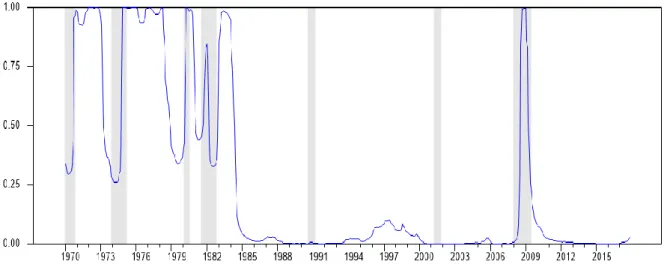
The inclusion of switches in volatility in the state equation of the model enables to distinguish four periods in the sample, as shown in Figure 1: a period of high macroeconomic volatility from 1970 to 1984, a period of low volatility from 1984 to 2007 corresponding to the Great Moderation, a second period of high macroeconomic volatility corresponding to the Great Recession (2007-2009), and a period of low volatility from the end of the Great Recession to the end of the sample (2009-2017). Looking at probabilities of being in a high-volatility regime (Figure 1), the transitions between the four periods are quite sharp. From Figure 1, we also conclude that the increase in volatility at the time of the Great Recession was only temporary and did not put an end to the Great Moderation, which is in line with Gadea-Rivas et al. (2018) and Charles et al. (2018). We also identify more minor fluctuations of the probability of being in a high-volatility state during the first period (1970-1984), something which is also noticed by Antolin-Diaz et al. (2017) who rely on a stochastic volatility specification.
Figure 1. Extended MS-DFM: Smoothed probability of being in a high-volatility
regime
Estimation sample: 1970M01-2017M12. Data vintage: 2017M12. Estimation based on 1 5000 draws of the Gibbs Sampler (the first 5 000 are discarded).
5.2. Improved detection of recessions when allowing for different characteristics of
expansions and recessions between volatility regimes
As shown in Figure 2, allowing for switches in volatility in the state equation and for different expansion and recession characteristics across volatility regimes also helps to better capture the two recessions that occurred during the Great Moderation period. This finding is in line with McConnell and Perez-Quiros (2000) who showed using a univariate MS-model that these two modelling features improved the detection of turning
points after the mid-1980s. We extend their findings to a multivariate context and a more recent sample.
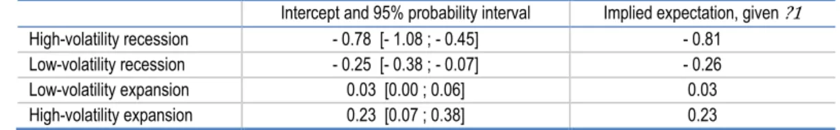
Estimation results are presented in Table 2. Looking at the intercept of the state equation, we notice that the discrepancy between high- and low-volatility recessions is twice bigger than between high-and low-volatility expansions. This asymmetry in the estimated impact of volatility on economic growth is consistent with the vulnerable growth dynamics recently put forward by Adrian et al. (2019). These authors show that deteriorating financial conditions, as measured by the National Financial Conditions Index (NFCI), are associated with both an increase in the conditional volatility and a decrease in the conditional mean of quarterly GDP growth in the US. They also show that this effect is asymmetric: the lower quantiles of the distribution of future GDP growth are strongly dependent on the tightness of financial conditions, whereas upper quantiles are stable over time. Looking at historical time series, it appears that financial conditions are precisely tighter than average before the Great Moderation and during the Great Recession (see Figure 2 in Adrian et al., 2019), i.e. when our model identifies a high-volatility regime.
Table 2. Intercept of the state equation, depending on the underlying regime
Intercept and 95% probability interval Implied expectation, given ?1
High-volatility recession - 0.78 [- 1.08 ; - 0.45] - 0.81 Low-volatility recession - 0.25 [- 0.38 ; - 0.07] - 0.26 Low-volatility expansion 0.03 [0.00 ; 0.06] 0.03 High-volatility expansion 0.23 [0.07 ; 0.38] 0.23 Note: Estimation sample: 1970M01-2017M12. Data vintage: 2017M12.
Figure 2. Influence of switching volatility on smoothed recession probabilities
Estimation sample: 1970M01-2017M12. Data vintage: 2017M12. Estimation based on 15 000 draws of the Gibbs Sampler (the first 5 000 are discarded).
MS-DFM Intercept refers to a model where volatility is not allowed to switch. Otherwise, this model has the same characteristics as the Extended MS-DFM.
5.3. Declining long-term GDP growth in the US since the turn of the century
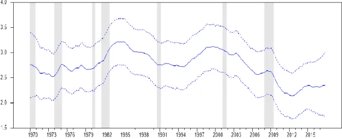
Similarly to Antolin-Diaz et al. (2017), we identify a decrease in the US long-term GDP growth which started in the early 2000s, i.e. before the Great Recession, and continued thereafter (see Figure 3). This result is compatible with the view that the Great Recession may have negatively affected the US trend growth rate and reinforced pre-existing factors. As compared to 2000, the estimated US long-term GDP growth is lower by around one percentage point per year in 2010 and seems to have stabilised since then. This slowdown in US long-term GDP growth follows an increase in the second half of the 1990s, which corresponds to a period of increase in US productivity growth (Jorgenson et al. 2008).
Figure 3. Extended MS-DFM: Smoothed estimate of the US annual long-run GDP
growth rate
Estimation sample: 1970M01-2017M12. Data vintage: 2017M12. Estimation based on 15 000 draws of the Gibbs Sampler (the first 5 000 are discarded).
Dashed lines delineate the 68% credibility interval.
5.4. Comparison of different model specifications based on DICs and marginal
likelihoods
The two refinements to the standard MS-DFM framework that we put forward in this paper are not only supported by the fact that they allow to capture changes in long-term GDP growth and to improve turning point detection. They are also supported by statistical criteria.
We first rely on the Deviance Information Criterion (DIC) to compare model specifications. This criterion has been specifically designed to compare complex hierarchical models like the one in this paper (Spiegelhalter et al., 2002). It is also used by Eo and Kim (2016). Like other information criteria, the DIC includes two terms, one capturing model fit and the other penalising for model complexity:
𝐷𝐼𝐶 = 𝐸⏟ 𝜃̃,𝑆̃,𝑉̃|𝑌[−2 ∙ log 𝑓(𝛥𝑦̃ |𝜃̃, 𝑆1..𝑇 ̃ , 𝑉1..𝑇 ̃ )]1..𝑇 𝐷𝑒𝑐𝑟𝑒𝑎𝑠𝑒𝑠 𝑤ℎ𝑒𝑛 𝑚𝑜𝑑𝑒𝑙 𝑓𝑖𝑡 𝑖𝑚𝑝𝑟𝑜𝑣𝑒𝑠 + 𝐸𝜃̃,𝑆̃,𝑉̃|𝑌[−2 ∙ log 𝑓(𝛥𝑦̃ |𝜃̃, 𝑆1..𝑇 ̃ , 𝑉1..𝑇 ̃ )] + 2 log 𝑓(𝛥𝑦1..𝑇 ̃ |𝜃̃1..𝑇 ∗, 𝑆̃1..𝑇 ∗ , 𝑉̃1..𝑇 ∗ ) ⏟ 𝑃𝑒𝑛𝑎𝑙𝑡𝑦 𝑓𝑜𝑟 𝑚𝑜𝑑𝑒𝑙 𝑐𝑜𝑚𝑝𝑙𝑒𝑥𝑖𝑡𝑦
In the above formula, 𝜃̃ corresponds to the vector of constant model parameters (e.g. autoregressive parameters), 𝜃̃∗ to their posterior mean, and 𝑓(𝛥𝑦̃ |𝜃̃, 𝑆1..𝑇 ̃ , 𝑉1..𝑇 ̃ ) to the 1..𝑇
model conditional likelihood. Model selection is based on the minimisation of the DIC. This information criterion is relatively easy to compute when model estimation is based on Bayesian Markov Chain Monte Carlo (MCMC) techniques, like Gibbs Sampling. Nevertheless, the literature shows that DIC estimation is all the more accurate that the number of parameters in the conditioning set of the log-likelihood is limited (Chan and Grant 2016). Here, we compute the conditional log-likelihood from the Kalman filter step of the Gibbs Sampler. In a nutshell, the Kalman filter estimates the expectation and variance of the model’s state vector, conditional on past observations and other model variables and parameters, which then allows to estimate log 𝑓(∆𝑦𝑡|𝛥𝑦̃ , 𝜃̃, 𝑆1..𝑡−1 ̃ , 𝑉1..𝑇 ̃ ) 1..𝑇
for each date t. 7 In this case, the conditioning set includes the two Markov variables 𝑆̃ 1..𝑇
and 𝑉̃ and all constant model parameters, but not the large state vector 𝛼1..𝑇 ̃. Summing 1..𝑇
these log-predictive likelihoods over time and averaging over posterior draws of the Gibbs Sampler finally gives an estimate of 𝐸𝜃̃,𝑆̃,𝑉̃|𝑌[−2 ∙ log 𝑓(𝛥𝑦̃ |𝜃̃, 𝑆1..𝑇 ̃ , 𝑉1..𝑇 ̃ )]. 1..𝑇
Alternatively, first averaging over posterior draws of the Gibbs Sampler, and then computing the predictive log-likelihoods with the Kalman filter allows to estimate log 𝑓(𝛥𝑦̃ |𝜃̃1..𝑇 ∗, 𝑆̃1..𝑇
∗
, 𝑉̃1..𝑇
∗
).
As an alternative to DICs which might be sensitive to the fact that the high-dimensional Markov variables are included in the conditioning set, we also compute marginal log-likelihoods for different model specifications. In this case, the preferred specification is the one with the highest marginal log-likelihood. As we did for DIC computations, we take advantage of the fact that, conditional on the two Markov variables, the MS-DFM is a linear Gaussian state-space model. Therefore, we can use the Kalman filter to compute 𝑓(∆𝑦𝑡|𝛥𝑦̃ , 𝜃̃1..𝑡−1 ∗, 𝑆̃ , 𝑉1..𝑡 ̃ ) for each date. The most difficult and time-consuming part of 1..𝑡
the marginal log-likelihood computation for this class of models is to numerically integrate out 𝑆̃ and 𝑉1..𝑡 ̃ from 𝑓(∆𝑦1..𝑡 𝑡|𝛥𝑦̃ , 𝜃̃1..𝑡−1 ∗, 𝑆̃ , 𝑉1..𝑡 ̃ ). To do so, we rely on a 1..𝑡
particle filter which provides us with a sample of N independent particles 𝑆̃1..𝑇
𝑛
and 𝑉̃1..𝑇
𝑛
(𝑛 = 1. . 𝑁). The underlying idea of the particle filter is to draw 𝑆̃1..𝑡
𝑛
and 𝑉̃1..𝑡
𝑛
, conditional on 𝛥𝑦̃ and 𝜃̃1..𝑡−1 ∗, using an importance sampling distribution which
approximates the true but unknown distribution of these variables. An important aspect of the particle filter is that it draws 𝑆̃1..𝑡
𝑛 and 𝑉̃1..𝑡 𝑛 recursively, based on 𝑆̃1..𝑡−1 𝑛 and 𝑉̃1..𝑡−1 𝑛 . This allows key computing efficiency gains. The general functioning of the particle filter and key issues such as the choice of the importance sampling distribution and the weighting of the particles are explained in detail in Annex G.
7
Note that given the structure of the model, the following equality applies 𝑓(∆𝑦𝑡|𝛥𝑦̃ , 𝜃̃, 𝑆1..𝑡−1 ̃ , 𝑉1..𝑇 ̃ ) = 𝑓(∆𝑦1..𝑇 𝑡|𝛥𝑦̃ , 𝜃̃, 𝑆1..𝑡−1 ̃ , 𝑉1..𝑡 ̃ ). 1..𝑡
This previous step gives us 𝑓(∆𝑦𝑡|𝛥𝑦̃ , 𝜃̃1..𝑡−1 ∗) for each date, from which we can
compute log 𝑓(𝛥𝑦̃ |𝜃̃1..𝑇 ∗). We finally rely on Chib’s (1995) formula to estimate the
marginal log-likelihood log 𝑓(𝛥𝑦̃ ) of each specification, as follows: 1..𝑇
log 𝑓(𝛥𝑦̃ ) = log 𝑓(𝛥𝑦1..𝑇 ̃ |𝜃̃1..𝑇 ∗) + log 𝜑(𝜃̃∗) − log 𝜑(𝜃̃∗|𝛥𝑦̃ ) 1..𝑇
As above, 𝜃̃∗ corresponds to the vector of constant model parameters evaluated at their posterior mean. log 𝜑(𝜃̃∗) and log 𝜑(𝜃̃∗|𝛥𝑦̃ ) are the log-prior and posterior densities 1..𝑇
of these parameters, respectively. Note that the use of a particle filter to reduce the dimension of the conditioning set prior to the use of Chib’s (1995) formula is key to ensure accurate results, as shown by Frühwirth-Schnatter and Wagner (2008).8
To the best of our knowledge, Kaufmann (2000) is the only other paper in the literature computing the marginal likelihood of MS-DFMs. However our framework is more complex than the framework of Kaufmann (2000) since we have included Markov-Switching volatility and time-varying growth rates. In this respect, the following results and the marginal likelihood computation method described in Annex G can be considered as additional contributions of the present paper.
8
An alternative to the use of the particle filter would be to apply Chib’s (1995) formula on log 𝑓(𝛥𝑦̃ |𝜃̃1..𝑇 ∗, 𝑆̃1..𝑇 ∗
, 𝑉̃1..𝑇 ∗
) directly. This would result in a ‘complete-data’ marginal likelihood estimator, which would be easier to compute than our proposed estimator. Nevertheless, Frühwirth-Schnatter and Wagner (2008) show that the complete-data marginal likelihood estimator can be extremely inaccurate and recommend not to use it.
Table 3 compares the DICs and marginal log-likelihoods of four model specifications: a linear DFM, a MS-DFM with Markov-Switching in the intercept of the state equation governing factor dynamics, a MS-DFM with Markov-Switching on the intercept and the volatility of shocks of this state equation, and the Extended MS-DFM with the two Markov-Switching features and a time-varying long-term GDP growth rate. All models have the same five observable variables as inputs (see Section 4). This Table shows that both Markov-Switching features reduce the DIC as compared to a linear DFM. This is especially true for the Markov-Switching volatility of shocks. However, allowing for time-variation in the long-term GDP growth rate does not further reduce the DIC. When it comes to the marginal log-likelihood, both Markov-Switching features also improve (i.e. increase) it and we note a further marginal improvement related to the inclusion of the time-varying long-term GDP growth rate into the model. Given the closeness of the DICs and marginal log-likelihoods for the last two models, it seems wise to consider that they cannot be distinguished with these statistical criteria.
Given that GDP is only one out of five observed variables, and that it is only observed once every three months, this could explain why the inclusion of a time-varying trend in the corresponding measurement equation is only marginally supported by the marginal log-likelihood. Focusing on the forecasting performance of GDP after the Great Recession will add further support to this feature (see Section 6).
Table 3. Comparison of model specifications based on DICs and marginal
log-likelihoods
Model specification DIC Marginal log-likelihood
Linear DFM 3 784.5 -1 929.4
MS-DFM with MS on intercept only 3 725.2 -1 910.8 MS-DFM with MS on intercept and volatility 3 612.2 -1 895.4 MS-DFM with MS on intercept and volatility, and time-varying long-term GDP growth
rate (i.e. extended MS-DFM) 3 631.7 -1 892.5 Note: In all cases, the posterior mean of model parameters is estimated based on 15 000 draws of the Gibbs Sampler, from which the first 5 000 are discarded. In addition, 500 particles are used for marginal log-likelihood computations (see Annex G for details). Sample: 1970M01-2017M12. Data vintage: 2017M12. The preferred specification is the one minimising the DIC and maximising the marginal log-likelihood. In each case, this specification is indicated in bold.
6. Real-time performance of the Extended MS-DFM specification over the last decade
(2007-2017)
In this section, we carry out a real-time assessment of our Extended MS-DFM using vintages of data available from January 2007 to January 2017. In this real-time analysis, we start the estimation by considering as a first sample January 1970 - December 2006, then we recursively add new data and re-estimate the model. However, the specification of the model remains unchanged.
6.1. Real-time estimation of the US long-term GDP growth rate
As already pointed out in the previous section, the decrease in the US long-term GDP growth rate that we estimate with our Extended model is about one percentage point per year compared to the early 2000s (see red curve in Figure 4, corresponding to the 2017M01 data vintage). It is interesting to notice that, over the same period, the professional forecasters surveyed by the Federal Reserve Bank of Philadelphia have revised their expectations of average GDP growth over the next 10 years by a similar amount, and that both estimates converge at the end of the sample.9
Figure 4 shows that the model needs some time to identify the drop in long-run GDP growth. Indeed, until 2010, the estimated long-run GDP growth is above 3% but progressively decreases from 2011 onwards (dashed curves in Figure 4). However, when compared with estimates provided by professional forecasters, it appears that the model-based real-time estimates converge more rapidly to the final estimate (red curve) than the SPF real-time estimates since 2011, which seem to be affected by some rigidities.
9
We use the variable RGDP10 in the Survey of Professional Forecasters (SPF). The corresponding question is asked only once a year, in January. This is why we compare the SPF with our model-based assessment using January data vintages.
Figure 4. Smoothed estimates of the US annual long-term GDP growth rate,
consecutive data vintages (2007M01 - 2017M01)
6.2. Real-time detection of the Great Recession
Whereas we relied on the 2017M12 data vintage in order to estimate recession probabilities in Section 5, we now rely on real-time data vintages in order to assess when the model detects the start and the end of the Great Recession.
There is no perfect consensus in the literature on when to formally announce that a recession has started or ended based on the recession probabilities estimated with Markov-Switching models. In the present paper where we use a mix of quarterly and monthly series, we rely on a decision rule which is very similar to the ones advocated by Chauvet and Piger (2008) and Hamilton (2011).10 We announce a recession when the probability of recession moves from below to above 0.7 and stays above 0.7 for three consecutive months, and we identify as the start of the recession the first month for which the probability of recession exceeds 0.5. Conversely, we announce that a recession is over when the probability of recession moves from above to below 0.3 and stays below 0.3 for
10
Hamilton (2011) suggests the following decision rule when relying on quarterly GDP data: “When the one-quarter smoothed inference 𝑃(𝑆𝑡|𝑦𝑡+1, 𝑦𝑡, . . , 𝑦1; 𝜃̂𝑡+1) first exceeds 0.65, declare that a recession has started, and at that time assign a probable starting point for the recession as the beginning of the most recent set of observations for which 𝑃(𝑆𝑡−𝑗|𝑦𝑡+1, 𝑦𝑡, . . , 𝑦1; 𝜃̂𝑡+1) exceeds 0.5.” Using only the four NBER monthly series to infer recession probabilities, Chauvet and Piger (2008) require that the probability of recession moves from below to above 0.8 and remains above 0.8 for three consecutive months before announcing a recession. Similarly to Hamilton (2011), they then identify as the start of the recession the first month for which the probability moves above 0.5.
three consecutive months, and we identify as the end of the recession the last month for which the probability is above 0.5.
Results are reported in Table 4. The start and end dates of the Great Recession identified by the Extended MS-DFM are in close agreement with those published by the NBER Business Cycle Dating Committee. Nevertheless, the model is able to announce the start and the end of the recession 2 and 11 months earlier than the NBER, respectively, thus allowing to integrate this information into GDP forecasts in a more timely way.
Table 4. Real-time dating of the Great Recession by the NBER and the Extended
MS-DFM
Peak date - NBER Extended MS-DFM Peak date - announcement - NBER Peak date Peak date announcement – Extended MS-DFM
2007 M12 (Start of the
Great Recession) 2007 M11 2008 M12 2008 M10 (-2m)
Trough date - NBER Extended MS-DFM Trough date - announcement - NBER Trough date Trough date announcement – Extended MS-DFM
2009 M06 (End of the
Great Recession) 2009 M06 2010 M09 2009 M10 (-11m)
6.3. Real-time forecasting performance of US quarterly GDP growth
We now focus on real-time GDP forecasting performance in order to highlight the relevance of the Extended MS-DFM specification, with Markov-Switching on the intercept and on the volatility of shocks in the equation governing factor dynamics, as well as a time-varying long-term GDP growth rate. The real-time forecasting performance of this specification is compared to the one of a fully linear DFM specification. The set of observed variables is the same in both cases.
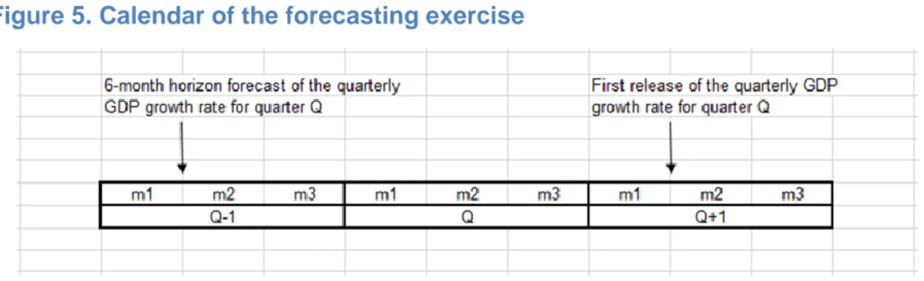
GDP forecasts for the current and the next quarters are produced at the end of each month, from six months up to one month before the quarterly GDP release date by the US Bureau of Economic Analysis (BEA). Given that quarterly GDP for quarter Q is released at the end of the first month of quarter (Q+1), 6-month horizon forecasts are produced at the end of the first month of quarter (Q-1), see Figure 5.
In practice, GDP forecasts are produced based on the first measurement equation of the state-space model. Supplementing the information set with missing data points up to the last month of the next quarter allows the simulation smoother to generate draws of the state vector up to this point, which in turn are used to compute forecasts of quarterly GDP growth. A sequence of forecasts is obtained for each iteration of the Gibbs sampler. These sequences of forecasts are finally averaged across draws to produce the final result.
Table 5 compares the real-time Root Mean Square Forecast Errors (RMSFEs) of our Extended MS-DFM and those stemming from a standard linear DFM using the same information set. We present the ratios of RMSFEs: a value below one means that the Extended MS-DFM outperforms the linear DFM. We focus on the Great Recession (2007Q4-2009Q2) and its aftermath (2011Q1-2017Q4), namely the two periods for which we expect regime switches and the time-varying long-term GDP growth rate to have the largest impact on the forecasting performance of the Extended MS-DFM. Figure 6 and Figure 7 compare the underlying point forecasts of the two models at 6-month and 1-month horizons, respectively. These forecasts underlie the RMSFEs shown in Table 5. In terms of RMSFEs, the Extended MS-DFM improves upon the linear DFM at horizons (M-5) and (M-6) in both sub-periods. At shorter horizons, the Extended MS-DFM only remains better than the linear DFM over 2011Q1-2017Q4, but not during the Great Recession.
The better forecasting performance of the Extended MS-DFM as compared to the linear DFM over 2011Q1-2017Q4 is related to the inclusion of the time-varying long-term GDP growth rate into the model. The fact that this feature has such an influence on forecasting performance suggests that the model tends to revert quite quickly to its unconditional mean. As announced in Section 5, focusing on GDP forecasting demonstrates the relevance of the time-varying long-term GDP growth rate even though the impact of this feature is less visible in the DIC and the marginal log-likelihood of the model. We explain this finding by the fact that this feature only plays a role for GDP in the model specification, whereas the DIC and the marginal log-likelihood take into account how the model fits the data for all five variables in the information set simultaneously.
This exercise also shows that the explicit identification of recession regimes helps to improve GDP forecasts six months before the GDP release date. Figure 6 makes it clear that this improvement could be even more substantial if the model were able to identify the start and the end of the Great Recession at earlier dates in real time. Note that the model information set only includes coincident and lagging variables at this stage (Section 4). At least in principle, it should be possible to further improve the detection of transitions between expansion and recession phases by adding leading variables in the model information set. We leave this as an avenue for further research.
Table 5. Relative RMSFEs of the Extended MS-DFM and the linear DFM (forecasts based on
real-time data)
(M-1) (M-2) (M-3) (M-4) (M-5) (M-6)
2007Q4-2009Q2 1.02 1.16 1.06 1.07 0.97 0.82
2011Q1-2017Q4 (0.22) 0.98 (0.07) 0.95* 0.85** (0.02) (0.11) 0.92 0.88** (0.04) (0.06) 0.90* Note: For the comparison over 2011Q1-2017Q4, values in brackets indicate p-values that the RMSFEs of the Extended MS-DFM and the linear DFM are drawn from the same data generating process (H0). Values below 0.1 indicate that H0 can be rejected at the 10% confidence level. These p-values are computed using the Harvey et al. (1997) small-sample correction of the Diebold and Mariano (1995) test statistic. As argued by Antolin-Diaz et al. (2017) based on Monte Carlo results in Clark and McCracken (2013), this pragmatic approach allows to reliably compare forecasts in cases where models are nested and forecasts are produced using expanding windows. The Great Recession sample (2007Q4-2009Q2) is too short to assess whether differences in forecasting performance between the two models are statistically significant or not.
Figure 6. Comparison of real-time point forecasts at a 6-month horizon: Linear
DFM vs. Extended MS-DFM specification
Figure 7. Comparison of real-time point forecasts at a 1-month horizon: linear
DFM vs. Extended MS-DFM specification
Finally, Figure 8 and Figure 9 show density forecasts produced by both models at horizons of 6 months. Note that the Bayesian estimation strategy adopted in this paper allows to incorporate all sources of uncertainty in these density forecasts, those related to the filtering of the underlying factor and of the business cycle and volatility states, as well as parameter uncertainties. As opposed to the linear DFM, whose average forecast and forecast uncertainty at a 6-month horizon remain roughly constant over time (Figure 9), the Extended MS-DFM produces a lower average forecast with a larger forecast uncertainty at the time of the Great Recession (Figure 8). It is mainly the left-hand side of the forecast distribution that shifts downwards in this case: low-growth outcomes become more likely when the model identifies a risk of recession, but the upper part of the forecast density remains roughly unchanged. This is in agreement with the vulnerable growth dynamics described by Adrian et al. (2019).
Figure 8. Real-time density forecasts at a 6-month horizon: Extended MS-DFM
7. Conclusion
In this paper, we put forward an extension of the standard Markov-Switching Dynamic Factor Model (MS-DFM) by accounting for two stylised facts of the US economy: changing macroeconomic volatility and fluctuations in the long-run GDP growth rate. This Extended MS-DFM comes as an innovation in the literature and could potentially be used for other advanced economies showing similar patterns.
We first show that the introduction of Markov-Switching volatility in the standard MS-DFM framework is supported by statistical criteria (DICs and marginal likelihoods), and largely improves the detection of turning points in the US business cycle during the Great Moderation. In addition, our Extended model shows evidence that the Great Moderation that started in the mid-1980s is not over, and that the Great Recession, beyond its effect on GDP growth, led to a temporary increase in macroeconomic volatility. The ability of the model to detect recessions in both high- and low-volatility environments is thus very relevant for the detection of future recessions.
As a second improvement to the standard MS-DFM framework, our model also incorporates a time-varying long-term GDP growth rate. This feature enables to identify a continuous decline in the US long-term GDP growth rate of around one percentage point per year as compared to the early 2000s. This result is in line with the empirical literature on the long-run decline in US potential growth. According to our model, about half of this loss occurred before the Great Recession. Nevertheless, the Great Recession may also have negatively affected the US trend growth rate and reinforced pre-existing factors. Overall, our Extended MS-DFM demonstrates that allowing for both regime switches and time-variation in long-term GDP growth is important to improve the accuracy of real-time short-term GDP forecasts since 2007. The first feature helps to improve GDP forecasts during the Great Recession while the second is most helpful in the aftermath of this recession. Being able to identify the start and the end of the Great Recession even earlier, e.g. through the use of leading variables, would allow to further improve the forecasting performance of the model during this and other recessions. We leave this as an avenue for further research.
References
Adrian, T., N. Boyarchenko and D. Giannone (2019), “Vulnerable growth”, American Economic Review, Vol. 109, No. 4, pp. 1263-1289.
An, Z., J.T. Jalles and P. Loungani (2018), “How well do economists forecast recessions?”, IMF Working
Paper, No. 18/39.
Antolin-Diaz, J., T. Drechsel and I. Petrella (2017), “Tracking the slowdown in long-run GDP growth”,
The Review of Economics and Statistics, Vol. 99, No. 2, pp. 343-356.
Bai, J. and P. Wang (2011), “Conditional Markov chain and its application in economic time series analysis”, Journal of Applied Econometrics, Vol. 26, pp. 715-734.
Bauwens, L. and J.V.K. Rombouts (2012), “On marginal likelihood computation in change-point models”, Computational Statistics and data Analysis, Vol. 56, pp. 3415-3429.
Burns, A.F. and W.C. Mitchell (1946), “Measuring business cycles”, National Bureau of Economic
Research.
Camacho, M., G. Perez-Quiros and P. Poncela (2018), “Markov-switching dynamic factor models in real time”, International Journal of Forecasting, Vol. 34, pp. 598-611.
Camacho, M., G. Perez-Quiros and P. Poncela (2014), “Green shoots and double dips in the Euro area: A real-time measure”, International Journal of Forecasting, Vol. 30, pp. 520-535.
Chan, J.C.C. and A.L. Grant (2016), “Fast computation of the deviance information criterion for latent variable models”, Computational Statistics and Data Analysis, Vol. 100, pp. 847-859.
Charles, A., O. Darné and L. Ferrara (2018), “Does the Great Recession imply the end of the Great Moderation? International evidence”, Economic Inquiry, Vol. 56, No. 2, pp. 745-760.
Chauvet, M., Z. Senyuz and E. Yoldas (2015), “What does financial volatility tell us about macroeconomic fluctuations?”, Journal of Economic Dynamics and Control, Vol. 52, pp. 340-360.
Chauvet, M. and Y. Su (2014), “Nonstationarities and Markov switching models”, in Ma and M. Wohar (eds.), Recent Advances in Estimating Nonlinear Models With Applications in Economics and Finance, Springer Science Business Media, New York.
Chauvet, M. and S. Potter (2013), “Forecasting output”, Handbook of Economic Forecasting, Chapter 3, pp. 141-194.
Chauvet, M. and J. Piger (2008), “A comparison of the real-time performance of two business-cycle dating methods”, Journal of Business and Economics Statistics, Vol. 26, No. 1, pp. 42-49.
Chauvet, M. and J.D. Hamilton (2005), “Dating business cycle turning points”, NBER Working Paper, Vol. 11422.
Chauvet, M. (1998), “An econometric characterization of business cycle dynamics with factor structure and regime switching”, International Economic Review, Vol. 39, No. 4, pp. 969-996.
Chib, S. (1995), “Marginal likelihood from the Gibbs output”, Journal of the American Statistical
Association, Vol. 90, pp. 1313-1321.
Clark, T.E. and M.W. McCracken (2013), “Advances in forecast evaluation”, Handbook of Economic
Forecasting, Chapter 20, pp. 1107-1201.
Review of Economics and Statistics, Vol. 78, No. 1, pp. 67-77.
Diebold, F.X. and R.S. Mariano (1995), “Comparing predictive accuracy”, Journal of Business and
Economic Statistics, Vol. 13, pp. 253-263.
Doucet, A. and A.M. Johansen (2011), “A tutorial on particle filtering and smoothing: Fifteen years later”,
Oxford Handbook of Nonlinear Filtering, pp. 656-704.
Durbin, J. and S.J. Koopman (2002), “A simple and efficient simulation smoother for state space time series analysis”, Biometrika, Vol. 89, No. 3, pp. 603-615.
Eo, Y. and J. Morley (2017), “Why has the US economy stagnated since the Great Recession?”, The
University of Sydney, Economics Working Paper Series, Vol. 2017-14.
Eo, Y. and C.-J. Kim (2016), “Markov-switching models with evolving regime-specific parameters: Are postwar booms or recessions all alike?”, The Review of Economics and Statistics, Vol. 98, No. 5, pp. 940-949.
Ferrara, L. and C. Marsilli (2017), “Global growth: Optimism for 2017?” EcoNotePad Banque de France,
https://blocnotesdeleco.banque-france.fr/en/blog-entry/global-growth-optimism-2017.
Fernald, J., R. Hall, J. Stock and M. Watson (2017), “The disappointing recovery of output after 2009”,
Brooking Papers in Economic Activity, Vol. 48, No. 1, pp. 1-81.
Frühwirth-Schnatter, S. and H. Wagner (2008), “Marginal likelihoods for non-Gaussian models using auxiliary mixture sampling”, Computational Statistics and Data Analysis, Vol. 52, pp. 4608-4624. Gadea-Rivas, M.D., A. Gomez-Loscos and G. Perez-Quiros (2018), “Great Moderation and Great
Recession: From plain sailing to stormy seas?” International Economic Review, Vol. 59, No. 4, pp. 2297-2321.
Gerlach, R., C. Carter and R. Kohn (2000), “Efficient Bayesian inference for dynamic mixture models”,
Journal of the American Statistical Association, Vol. 95, pp. 819-828.
Giordani, P., R. Kohn and D. van Dijk (2007), “A unified approach to nonlinearity, structural change, and outliers”, Journal of Econometrics, Vol. 137, pp. 112-133.
Hamilton, J. (2011), “Calling recessions in real time”, International Journal of Forecasting, Vol. 27, pp. 1006-1026.
Hamilton, J. (1989), “A new approach to the economic analysis of nonstationary time series and the business cycle”, Econometrica, Vol. 57, No. 2, 357-384.
Harding, D. and A. Pagan (2006), “Synchronization of cycles”, Journal of Econometrics, Vol. 132, pp. 79.
Harvey, D., S. Leybourne and P. Newbold (1997), “Testing the equality of prediction mean square errors”,
International Journal of Forecasting, Vol. 13, pp. 281-291.
Jorgenson, D.W., M.S. Ho and K.J. Stiroh (2008), “A retrospective look at the US productivity growth resurgence”, Journal of Economic Perspectives, Vol. 22, No. 1, pp. 3-24.
Kaufmann, S. (2000), “Measuring business cycles with a dynamic Markov-switching factor model: An assessment using Bayesian simulation methods”, Econometrics Journal, Vol. 3, pp. 39-65.
Kim, C.J. and C.R. Nelson (1998), “Business cycle turning points, a new coincident index and tests of duration dependence based on a dynamic factor model with regime switching”, The Review of
Economics and Statistics, Vol. 80, No. 2, pp. 188-201.
Koopman, S.-J. and J. Durbin (2003), “Filtering and smoothing of state vector for diffuse state-space models”, Journal of Time Series Analysis, Vol. 24, No. 1, pp. 85-98.
Koopman, S.J. and J. Durbin (2000), “Fast filtering and smoothing for multivariate state space models”,
Journal of Time Series Analysis, Vol. 21, No. 3, pp. 281-296.
Lewis, C. and N. Pain (2015), “Lessons from OECD forecasts during and after the financial crisis”, OECD
Journal: Economic Studies, Vol. 2014, No. 1, pp. 9-39.
Marcellino, M., M. Porqueddu and F. Venditti (2016), “Short-term forecasting with a mixed-frequency dynamic factor model with stochastic volatility”, Journal of Business and Economic Statistics, Vol. 34, No. 1, pp. 118-127.
Mariano, R. and Y. Murasawa (2003), “A new coincident index of business cycles based on monthly and quarterly series”, Journal of Applied Econometrics, Vol. 18, pp. 427-443.
McConnell, M.M. and G. Perez-Quiros (2000), “Output fluctuations in the United States: What has changed since the early 1980s?” American Economic Review, Vol. 90, No. 5, pp. 1464-1476.
McCracken, M.W. and S. Ng (2016), “FRED-MD: A monthly database for macroeconomic research”,
Journal of Business and Economic Statistics, Vol. 34, No. 4, pp. 574-589.
OECD (2013), “Well-Being and the Global Financial Crisis”, in How’s Life? 2013: Measuring Well-Being.
OECD Publishing, Paris. https://doi.org/10.1787/how_life-2013-7-en.
Sensier, M. and D. van Dijk (2004), “Testing for volatility changes in US macroeconomic time series”,
The Review of Economics and Statistics, Vol. 86, No. 3, pp. 833-839.
Spiegelhalter, D.J., N.G. Best, B.P. Carlin and A. van der Linde (2002), “Bayesian measures of model complexity and fit”, Journal of the Royal Statistical Society, Series B, Vol. 64, pp. 583-639.
Stiglitz, J.E., J-P. Fitoussi and M. Durand (2018), “Beyond GDP: Measuring What Counts for Economic and Social Performance”, OECD Publishing, Paris. https://doi.org/10.1787/9789264307292-en.
Stock, J.H. and M.W. Watson (2012), “Disentangling the channels of the 2007-2009 recession”,
Brookings Papers on Economic Activity, Spring 2012, pp. 81-156.
Stock, J.H. and M.W. Watson (2002), “Has the business cycle changed and why?”, NBER
Macroeconomics Annual, MIT Press, pp. 159-230.
Stock, J.H. and M.W. Watson (1989), “New indexes of coincident and leading economic indicators”,