mixture, depending on three parameters (high and low reflector variances and reflector density), on the wavelet impulse response, and on the observation noise variance. These parameters are unknown and must be estimated from the recorded trace, which is the reflectivity convolved with the wavelet, plus noise. Two methods are compared in this paper for the parameter estimation. Since we are considering an incomplete data problem, we first consider maximum likelihood estimation by means of a stochastic expectation maximization (SEM) method. Alternatively, proper prior distributions can be specified for all unknown quantities. Then, a Bayesian strategy is applied, based on a Monte Carlo Markov Chain (MCMC) method. Having estimated the parame-ters, one can proceed to the deconvolution. A maximum posterior mode (MPM) criterion is optimized by means of an MCMC method. The deconvolution capability of these procedures is checked first on synthetic signals and then on the seismic data of the IFREMER ESSR4 campaign, where the wavelet duration blurs the reflectivity, and on the SMAVH high-resolution marine seismic data.
Index Terms—Blind deconvolution, EM algorithm, Markov Chain Monte Carlo (MCMC), maximum likelihood, maximum posterior mode (MPM) method, seismic signals, stochastic expec-tation maximization (SEM) algorithm.
I. INTRODUCTION
T
HE AIM of high-resolution marine seismic exploration is to obtain an image of the sea-bottom lithography from reflected acoustic waves emitted by various seismic sources. It uses high-frequency waves with frequencies ranging from 500 Hz to 2 KHz, which penetrates in the ground as far as 100 m with a resolution of 1 m. The seismic source, which produces the seismic wavelet, is tracked by a ship Fig. 1, which also drags a multitrace streamer consisting in an array of hydrophones. The hydrophones record the reflected acoustic signals. The traveling distance between two shots is equal to the half of the distance between two sensors, which means that each sensor will receive signals coming from the same common reflection point of the sea bed during a shot sequence. This allows to average the sig-nals to increase the signal-to-noise ratio (SNR). The received signals can be modeled as the convolution of a source wavelet and a reflectivity sequence, which describes the most impor-tant interfaces met by the emitted wave [1]. The source waveletManuscript received July 1, 2002; revised March 11, 2003.
The authors are with the ENST Bretagne, Brest Cedex 29285, France (e-mail: jm.boucher@enst-bretagne.fr).
Digital Object Identifier 10.1109/JOE.2003.816683
phenomenon due to multiple reflections on the free sea surface and also by averaging hydrophone signals in the common point method; the layered geological structure of the sea bottom acts as a lowpass filter, depending on the localization of the common point. Furthermore, the problem can be modeled as the filtering of the reflectivity sequence by a lowpass filter, whose impulse response is the wavelet source. So, since the wavelet is un-known, blind deconvolution must be applied to recover the re-flectivity sequence from the recorded trace.
The first deconvolution methods [2], [3] assumed that the reflectivity sequence was a white noise and that the wavelet was described by a deterministic ARMA model. In this case, usual parametric methods based on second-order statistics can be used, but they systematically lead to a minimum phase solution. If the wavelet is nonminimum phase, which occurs in most experiments, one may then use higher order statistics (third- or fourth-order cumulants in general) to retrieve the signal phase [4], [5]. However, this kind of techniques requires a large amount of data to ensure efficient estimation. Such conditions are not satisfied in marine reflection seismology, where the observation vectors contain less than 1000 samples. Moreover, these higher order approaches do not really take into account the statistical information contained in the reflectivity signal. In particular, one simple way to characterize the seismic signal is to consider that the sea floor is composed of several layers that are more or less homogenous and separated by interfaces where the reflections occur. This simple hypothesis permits us to statistically model the reflectivity sequence as a Bernoulli–Gaussian process [6], [7] or, more generally, as a mixture of Gaussian distributions [8]. For each sample of the reflectivity sequence, a Bernoulli variable characterizes the presence or the absence of a reflector. Then, conditionally to that label, the amplitudes follow a Gaussian distribution. Once this type of a priori information is given, it is easy to incorporate it into the convolution model.
The estimation can then be achieved by maximizing the pos-terior likelihood functional. In practice, maximizing the likeli-hood functional of incomplete data models (here, the model is completed by incorporating the Bernoulli reflectivity sequence) can be done by using the expectation–maximization (EM) al-gorithm [9]. However, for our problem, this alal-gorithm requires high-dimensional integrations that are very difficult to calcu-late by means of classical numerical methods. MCMC methods
Fig. 1. Acquisition system.
Fig. 2. Synthetic trace.
[15] enable us to circumvent this difficulty by solving the inte-gration and optimization problems by simulating random vari-ables. This approach leads to stochastic versions of the EM al-gorithm [stochastic expectation maximization (SEM), SAEM] [12]. Moreover, we investigate the problem in a totally Bayesian framework in which prior information is introduced upon the pa-rameters [10]. Then, the estimation of the Bernoulli–Gaussian model and of the wavelet is solved by the simulation of random variables via MCMC algorithms such as the Gibbs sampler [10]. Once the model has been estimated, the next step is the de-convolution itself. This problem is said to be “ill-posed” be-cause, in the presence of noise, different reflectivity sequences can lead to similar seismic data. Therefore, it is necessary to use as much prior information as possible upon the reflectivity to limit the set of acceptable solutions. Thus, it is natural to ac-count for the Bernoulli–Gaussian assumption introduced above. Then, we need an adequate procedure to achieve the detection of reflectors and the estimation of their amplitude. Actually, the problem can be solved using either the maximum a posteriori (MAP) criterion, which can be optimized using the simulated annealing technique, or by the suboptimum maximum posterior mode (MPM) method, which involves optimization by means of a MCMC technique.
II. PROBLEMMODELING
A seismic trace can be modeled as the convolution of the un-known wavelet with the reflectivity sequence , yielding the observation
(1) and will, respectively, denote the trace vector of dimension N and the reflectivity sequence of length N. The source wavelet is represented by a moving average (MA) model with L coef-ficients. The noise is assumed to be white Gaussian with vari-ance . The reflectivity is represented by two random variables , which define a generalized Bernouilli–Gaussian process [1]. If is equal to one, it indicates the position of a high reflector position and a small reflector position for zero. is the amplitude of the reflected signal and its distribution is a Gaussian mixture.
(2) (3) is the density of the reflectivity sequence. is the variance of high reflectors, while represents the variance of secondary reflections due to the inhomogeneity of each layer. It is assumed
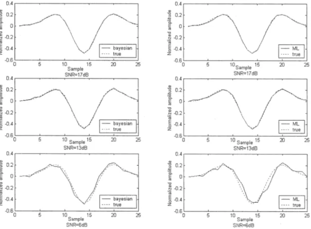
Fig. 3. True and estimated wavelets by using maximum likelihood (right images) and Bayesian methods (left images) for various SNR (from top to bottom: 17, 13, and 6 db).
The aim of the problem is to estimate
from the data and then to proceed to the deconvolution with the estimated source wavelet .
III. PARAMETERESTIMATION
A. Maximum Likelihood Approach
A classical method consists in using the maximum likelihood (ML) criterion as follows:
(4) As mentioned above, this is in fact an incomplete data problem [8], [9] and it must be solved by introducing the missing variables . The joint probability density is expressed by
(5) As , it can also be written as
(6) Each component of this equation can be easily expressed. As
is a Bernoulli variable, with
(7)
The variables are independent conditionally to the vari-ables
(8)
(9)
The complete Log likelihood is expressed by
(10)
with diag , , ,
. We note that , where and are
the convolution matrices associated with and .
When the complete data are known, the optimization problem solution is straightforward. A Gibbs sampler [10], [11] is used to obtain the complete data by simulation, which consists of a random sampling from the probability distribution , where means all the vector values except
TABLE I
PERFORMANCES OF THEBAYESIAN ANDML DECONVOLUTIONMSEw MEANSQUAREERRORBETWEENTRUE ANDESTIMATEDWAVELETS. MSEr MEANSQUARE
ERRORBETWEENTRUE ANDESTIMATEDIMPULSES OF THEREFLECTIVITYSEQUENCEFA NUMBER OFFALSEALARMS(DETECTEDIMPULSES OF
HIGH-AMPLITUDE,WHICH DO NOTEXIST). D = NUMBER OFDETECTEDIMPULSES OFHIGHAMPLITUDE(ON25 GENERATEDIMPULSES), LE1 = NUMBER OF
IMPULSESWHOSELOCALIZATION HAS ANERROR OFONESAMPLELEFT ORRIGHT, LE2 = NUMBER OFIMPULSESWHOSELOCALIZATION HAS ANERROR OFTWOSAMPLESLEFT ORRIGHT, LE3 = NUMBER OFIMPULSESWHOSELOCALIZATION HAS ANERROR OFTHREESAMPLESLEFT ORRIGHT
. In this case, it can be shown that the posterior density function becomes [8]
(11)
with
(12)
For the simulation of the vector , the Gibbs sampler has the following iterative steps:
For and
• Choice of k;
• Computation of ;
• Random sampling of in [0,1] and new value of :
• if
if ;
• Estimation: simulation of with ;
• New value: :
The SEM [12] is then used to solve the estimation problem:
Initialization:
• choice of and ;
For :
• E step:
• Simulation of by the Gibbs sampler
ac-cording to ;
• M step:
• Estimation of the parameters with
B. Bayesian Approach
In Bayesian estimation, the hyper parameters are random and have a prior density . When no prior distribution is available, it is possible to specify noninformative prior distributions that are easy to handle, such as conjugate priors [10]. Then, the objective is to estimate the joint posterior distribution , which can be expressed by using the Bays rule by
(13)
with
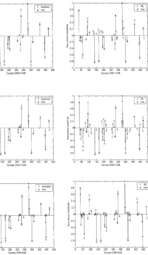
Fig. 4. True reflectivity and reflectivities.
This requires integrations that are generally impossible to perform. To overcome this difficulty, Monte Carlo methods are used to build a Markov chain whose equilibrium distribution coincides with the desired joint posterior distribution of the unknown parameters. This is performed by the Gibbs sampler,
which generates estimates by sampling from conditional distributions.
A detection–estimation procedure is used to simulate the missing variable, because the direct sampling from
Fig. 5. Convergence speed of the SEM method(SNR = 15 dB).
Fig. 6. Convergence speed for the Bayesian method(SNR = 15 dB).
• Detection: simulate according to the distribution , where any vector is defined by
• Estimation: simulate according to .
Each parameter is associated to a prior and classical conjugate priors, such as Gaussian distributions ; Beta distributions or Inverse Gamma distributions are used [10]
(15)
(16) (17) (18) The posterior distribution of is expressed by
(19) where
Fig. 7. Registered seismic trace n 1.
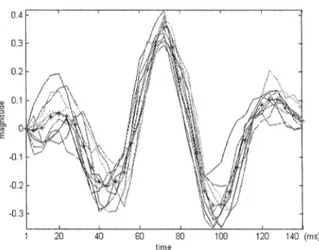
Fig. 8. Estimated wavelets of ten successive traces from 1 to 10 of shot 602 by maximum likelihood with the maximum value position atd = 68 ms.
and
(21) The posterior distribution of the noise variance is an Inverse Gamma distribution, as follows:
(22)
with
(23)
The posterior distribution of the primary reflectivity variance follows:
(24) with
(25)
Fig. 9. Estimated wavelets of ten successive traces from 1 to 10 of shot 602 by Bayesian method with the maximum value position atd = 68 ms.
The posterior distribution of the secondary reflectivity variance follows:
(26) with
(27)
The density of the reflectivity is given by
(28) with
(29)
From these distributions, an algorithm [13] similar to the Gibbs sampler leads to the parameter estimation
Random initialization of and ;
For ,
• simulate from • simulate from
Fig. 10. Convergence speed for the SEM method.
Fig. 11. Convergence speed for the Bayesian method.
• simulate from
• simulate from
• simulate from
• simulate from .
IV. DECONVOLUTION
As the parameters and, in particular, are now known, the deconvolution problem is reduced to an estimation of the hidden variables from the observation. The a posteriori log likelihood
is expressed by .
The separation principle [1] allows us to solve this maximiza-tion problem in two steps:
(30) (31) The estimation step leads to a mean square method because it is a quadratic form when is fixed
with and
Fig. 12. Estimated reflectivity sequence corresponding to trace n 1.
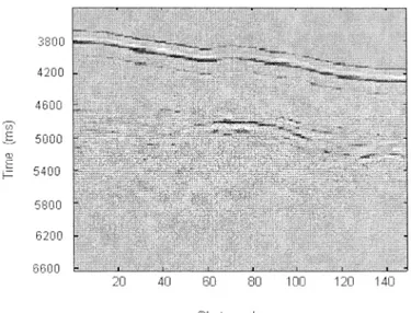
Fig. 13. Seismic image of ESSR4 data.
Fig. 14. Deconvolved image of ESSR4 data.
The detection problem is not so easy because the vector has discrete configurations, and testing all of them is not possible. The solution consists in the applying a simpler criterion called the maximum posterior mode (MPM) [14], which maximizes the marginal distribution . As it cannot be explicitly optimized, it is simulated by means of a Monte Carlo method
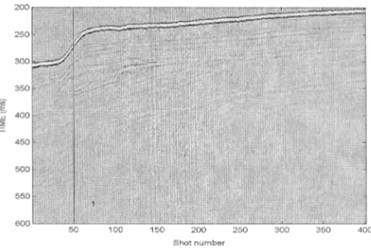
Fig. 15. Seismic image with SMAVH data.
using the Gibbs sampler. At each iteration, a sequence is generated according to the distribution .
The MPM algorithm follows the steps: 1) Initialization:
• Choice of and ;
2) Iteration with a learning period and a
steady-stage period ;
• Computation of
• Detection: random sampling of U in [0,1] if
elsewhere
• Estimation: random uniform sampling of with if if 3) Decision for ; • Detection if elsewhere • Estimation if if V. APPLICATION A. Synthetic Traces
We build a synthetic trace (Fig. 2) by convolving a white
Gaussian mixture impulse signal ( , ,
) with a synthetic Ricker wavelet (Fig. 3), plus additive white noise, whose variance is adjusted to obtain a variable SNR. The SNR is defined as
SNR
where stands for the wavelet energy.
In this simulation, 25 impulses of high amplitude corre-sponding to high reflectors were generated. We compare the deconvolution performances of the two methods with respect
Fig. 16. Deconvolved image with SMAVH data.
to SNR. Fig. 3 shows the true and estimated wavelets. It can be seen in Table I that the error MSEw is a bit higher with the ML method than with the Bayesian method at each SNR.
After applying the algorithms, it may occur that two neigh-boring estimated impulses are found, either successive or sepa-rated by one sample. Then, a postprocessing procedure must be used to fuse these impulses by replacing them by their gravity center. Fig. 4 shows the deconvolved reflectivity sequences and the true reflectivity sequence for both algorithms at SNR 17, 13, and 6 db. Table I compares the performances of the ML and Bayesian approaches for the reflectivity sequence in terms of good detection, false alarms, localization errors, and estimation error of the amplitude of detected impulses.
It can be seen on this example that the MCMC method gives a better deconvolution than the ML method. At high SNR, the localization of impulses by MCMC is more accurate with less misses and false detection than by ML, where more false detections occur. If SNR decreases, the impulse miss number increases, because low-amplitude impulses are not detected. High-amplitude impulses continue to be well localized. It can be remarked that both methods show good robustness with regard to the SNR decrease.
The SEM convergence speed of the parameters is shown in Fig. 5 for a SNR of 15 db. The convergence speed of the Bayesian approach is shown in Fig. 6. In this last case, the prior
distribution parameters were , ,
, , and .
We remark that it is faster for the Bayesian method, while the parameter variance is higher. The wavelet estimation is more accurate with the Bayesian method when the SNR decreases. B. Real Traces
1) ESSR4 Data: In the case of the ESSR4 data acquired during the ZAIANGO campaign by the IFREMER, the seismic
Fig. 17. Seismic trace along line 1 with SMAVH data.
data set was obtained using an innovative manner for synchro-nizing a cluster of GI guns in order to achieve deeper penetra-tion. The sources are no more synchronized on their firing order but on their time of maximum energy, therefore decreasing the signal bandwidth but increasing significantly the low-frequency content and, thus, the penetration. The source was composed of 11 synchronized airguns shooting every 20 s with a source wavelet whose spectrum is in the band of 0–128 Hz. The multi-trace streamer was composed of 360 clusters of 16 hydrophones, whose role was to improve the SNR by summing the received signals. The length of the steamer was 4.5 km and each hy-drophone cluster was separated by 12.5 m. The sampling rate was 4 ms and each trace was composed of 2500 samples (Fig. 7). The length of the MA model is a parameter that must be fixed. In our case, sufficient knowledge about the source wavelet gen-eration suggested the choice of a MA model with 35 coeffi-cients, giving a source duration of 140 ms.
When estimating the source wavelet, a problem of phase shift occurs because the convolution of shifted versions of the esti-mated wavelet with the reflectivity shifted the other way lead to the same seismic trace. As the wavelet is modeled by an MA process, there are some differences in the estimation when the position of the wavelet maximum value is changed. We assume that this position belongs to the interval. Then, the following al-gorithm is applied for neighboring traces, where the hypothesis of the wavelet stationary is made .
For trace :
• Wavelet estimation of with the hypothesis that the maximum is at position ;
• For
• Wavelet shift of one sample of toward the right;
• Wavelet estimation of ; For trace
• Wavelet estimation with an initialization by for The decision is given by the minimum of variance, which gives
Fig. 18. Estimated reflectivity sequence along line 1 with SMAVH data.
In this experiment, all maximum positions from 20 to 80 ms are explored with a step of 8 ms. The minimum variance is ob-tained for with a superposition of ten estimated wavelets from neighboring traces at the same maximum value. The ML wavelet estimation for the seismic trace of Fig. 7 is shown in Fig. 8. The Bayesian approach is presented in Fig. 9. The learning time has been experimentally set to 700 iterations. We remark that the variance of the estimated wavelet is lower with the Bayesian approach than with the ML approach, which suggests that introducing a prior knowledge regularizes estima-tion. The empirical mean of the other parameters is computed from the next 400 samples. The convergence speed of these pa-rameters for the ML and Bayesian methods is, respectively, in Figs. 10 and 11.
After convergence, we remark a higher variance of the param-eters with the Bayesian method. One reason for this is that the Bayesian approach uses simulations from probability distribu-tions more extensively than the ML approach. Nevertheless, the estimation means are similar. Fig. 12. shows the reflectivity se-quence obtained by applying the MPM deconvolution method.
Putting the traces of all the shots of the same hydrophone cluster side by side gives an image of the sea bottom stratigraphy (Figs. 13 and 14). Transitions between layers are thinner and less blurred in the deconvolved image.
2) High-Resolution SMAVH Data: These data come from a high-resolution marine seismic experiment undertaken by IFREMER in shallow water. The source is an air gun whose bandwidth is 200 Hz. The streamer is composed of 24 hydrophones separated by a length of 25 m. Fig. 15 shows the seismic image obtained from 401 successive shots. The MCMC algorithm is applied on the raw data and the estimated parameters are given in Table II. Fig. 16 shows the deconvolved image. Figs. 17 and 18 show, respectively, a raw seismic trace and the corresponding estimated reflectivity sequence along the vertical line 1. Comparing Figs. 15 and 16 shows that blind deconvolution improves the information quality given by the seismic image: New layers, which were blurred in the seismic image, appear clearly in the deconvolved image; layer interfaces are thinner and better localized in the deconvolved image. A contribution of blind deconvolution here is to let appear layers immediately under the sea-floor line, which were masked in the original image because of the high energy of the sea-floor reflection. This can also be seen by comparing Figs. 17 and 18.
the deconvolved image.
ACKNOWLEDGMENT
The authors gratefully thank J. Meunier, H. Nouzé, and B. Marsset from IFREMER for providing data and for their help in result interpretation.
REFERENCES
[1] J. M. Mendel, Maximum-Likelihood Deconvolution: A Journey Into Model-Based Signal Processing. Berlin, Germany: Springer-Verlag, 1990.
[2] E. A. Robinson, “Predictive decomposition of seismic traces,” Geophys., vol. 22, no. 4, pp. 767–778, 1957.
[3] J. M. Mendel, Optimal Seismic Deconvolution: An Estimation-Based Approach. New York: Academic, 1983.
[4] G. D. Lazear, “Mixed-phase wavelet estimation using fourth-order cu-mulants,” Geophys., vol. 58, no. 7, pp. 1042–1049, 1993.
[5] M. Boujida and J. M. Boucher, “Higher order statistics applied to wavelet identification of marine seismic signal,” in Proc. 8th Eur. Signal Process. Conf., vol. 1, 1996, pp. 137–141.
[6] Q. Cheng, R. Chen, and T. Li, “Simultaneous wavelet estimation and de-convolution of reflection seismic signals,” IEEE Trans. Geosci. Remote Sensing, vol. 34, pp. 377–384, Mar. 1996.
[7] J. Kormylo and J. M. Mendel, “Maximum-likelihood detection and esti-mation of Bernouilli-Gaussian processes,” IEEE Trans. Inform. Theory, vol. IT-28, pp. 482–488, 1982.
[8] M. Lavielle, “A stochastic algorithm for parametric and nonparametric estimation in the case of incomplete data,” Signal Process., vol. 42, pp. 3–17, 1995.
[9] A. P. Dempster, N. M. Laird, and D. B. Rubin, “Maximum likelihood from incomplete data via the EM algorithm,” J. R. Statist. Soc. Ser., vol. B-39, pp. 1–38, 1977.
[10] C. P. Robert, The Bayesian Choice. New York: Springer-Verlag, 1994. [11] S. Geman and D. Geman, “Stochastic relaxation, Gibbs distribution and the bayesian restoration of images,” IEEE Trans. Pattern Anal. Machine Intell., vol. 6, pp. 721–741, 1984.
[12] G. Celeux and J. Diebolt, “A stochastic approximation type EM algo-rithm for the mixture problem,” Stochastics Stochastics Rep., vol. 41, pp. 119–134, 1992.
[13] A. Doucet and P. Duvaut, “Bayesian estimation of state-space models applied to deconvolution of Bernouilli-Gaussian processes,” Signal Process., vol. 57, pp. 147–161, 1997.
[14] B. Chalmond, “An iterative Gibbsian technique for reconstruction of m-ary images,” Pattern Recognit., vol. 22, pp. 747–761, June 1989.
Jean-Marc Boucher (M’84) was born in 1952
and received the engineering degree in Telecom-munications from the Ecole Nationale Supérieure des telecommunications, Paris, France in 1975 and the Habilitation à Diriger des Recherches Degree in 1995 from the University of Rennes 1, Rennes, France.
He is currently a Professor in the department of signal and communications, Ecole Nationale Superieure des Telecommunications de Bretagne, Brest, France, where he is also Education Deputy Director. His current research interests include estimation theory, Markov models and Gibbs fields, blind deconvolution, wavelets, and multiscale image analysis with applications to radar and sonar image filtering and classifica-tion, multisensor seismic signal deconvoluclassifica-tion, electrocardiographic signal processing, and speech coding. He has published approximately 100 technical articles in these areas in international journals and conferences.
Benayad Nsiri (S’01) was born in Temara, Morocco,
in 1974. He received the D.E.A (French equivalent of M.Sc.) degree in electronics from the University of Bretagne Occidentale, Brest, France, in 2000. He is currently pursuing the Ph.D. at Ecole National Supérieure des Télécommunications de Bretagne, Brest, France
His research interests include signal processing, blind deconvolution, MCMC methods, seismic data, and higher order statistics.
Thierry Chonavel (M’97) received the Ph.D. degree
from Ecole Nationale Supérieure des Télécommu-nications, Paris, France, in 1992. His Ph.D. thesis was about bandlimited spectrum modeling and estimation, with applications to array processing.
He is currently a Professor at Ecole Nationale Supérieure des Télécommunications de Bretagne, Brest, France. His main research areas are in parameter estimation and adaptive techniques with applications to underwater acoustic tomography, seismic deconvolution, and mobile communications.