Hybridizing rapidly growing random trees and basin hopping yields an improved exploration of energy landscapes

(1)

HAL Id: hal-01191028

https://hal.inria.fr/hal-01191028

Submitted on 1 Sep 2015

HAL is a multi-disciplinary open access

archive for the deposit and dissemination of

sci-entific research documents, whether they are

pub-lished or not. The documents may come from

teaching and research institutions in France or

L’archive ouverte pluridisciplinaire HAL, est

destinée au dépôt et à la diffusion de documents

scientifiques de niveau recherche, publiés ou non,

émanant des établissements d’enseignement et de

recherche français ou étrangers, des laboratoires

hopping yields an improved exploration of energy

landscapes

Christine–Andrea Roth, Tom Dreyfus, Charles H. Robert, Frédéric Cazals

To cite this version:

Christine–Andrea Roth, Tom Dreyfus, Charles H. Robert, Frédéric Cazals. Hybridizing rapidly

grow-ing random trees and basin hoppgrow-ing yields an improved exploration of energy landscapes. [Research

Report] RR-8768, Inria. 2015, pp.29. �hal-01191028�

(2)

ISSN 0249-6399 ISRN INRIA/RR--8768--FR+ENG

RESEARCH

REPORT

N° 8768

September 2015 Project-Team

Algorithms-growing random trees

and basin hopping yields

an improved exploration

of energy landscapes

(3)

(4)

RESEARCH CENTRE

SOPHIA ANTIPOLIS – MÉDITERRANÉE

exploration of energy landscapes

A. Roth

∗

and T. Dreyfus

†

and C. H. Robert

‡

and F. Cazals

§

Project-Team Algorithms-Biology-Structure (ABS)

Research Report n° 8768 — September 2015 — 26 pages

Abstract: The number of local minima of the PEL of molecular systems generally grows

exponentially with the number of degrees of freedom, so that a crucial property of PEL exploration algorithms is their ability to identify local minima which are low lying and diverse.

In this work, we present a new exploration algorithm, retaining the ability of basin hopping (BH) to identify local minima, and that of transition based rapidly growing random trees (T-RRT) to foster the exploration of yet unexplored regions. This ability is obtained by interleaving calls to the extension procedures of BH and T-RRT, and we show tuning the balance between these two types of calls allows the algorithm to focus on low lying regions. Computational efficiency is obtained using state-of-the art data structures, in particular for searching approximate nearest neighbors in metric spaces.

We present results for the BLN69, a protein model whose conformational space has dimension 207 and whose PEL has been studied exhaustively. On this system, we show that the propensity of our algorithm to explore low lying regions of the landscape significantly outperforms those of BH and T-RRT.

Key-words: energy landscape exploration, sampling, local minima enumeration, basin hopping,

rapidly growing random trees, high dimensional spaces

∗_{Inria ABS}

†_{Inria ABS}

‡_{IBPC-LBT/CNRS. email: robert@ibpc.fr}

(5)

paysages ´

energ´

etiques

Résumé : Le nombre de minima locaux d’une surface d’énergie potentielle croˆıt généralement

exponentiellement en le nombre de degrés de liberté du système, de telle sorte qu’une propriété

critique des algorithmes d’exploration est leur aptitude `a identifier des minima de basse ´energie

et non redondants.

Dans ce travail, nous pr´esentons un nouvel algorithme d’exploration, ayant l’aptitude de basin

hopping `a identifier les minima locaux, et celle de transition based rapidly growing random trees

(T-RRT) à favoriser l’exploration de régions vierges. Ces propriétés sont obtenues en combinant

des appels aux proc´edures d’extension de BH et de T-RRT, et nous montrons que l’importance

relative entre ces deux types d’extensions permet `a notre algorithme de se focaliser sur les r´egions

de basse énergie. L’efficacité de l’algorithme est obtenue en utilisant des structures de données

pour la recherche de voisins approch´es dans les espaces m´etriques.

Nous présentons des résultats pour BLN69, un modèle de protéine dont l’espace

conforma-tionel est de dimension 207, et dont le paysage énergétique a été étudié de fa¸con exhaustive. Sur

ce système, nous montrons que notre algorithme identifie les régions de basse énergie de fa¸con

plus significative que les m´ethodes dont il est issu, a savoir BH and T-RRT.

Mots-clés : exploration de paysages énergétiques, échantillonage, énumération de minima

(6)

1 Introduction

Interpreting the physical-chemical behavior and the function of biological macromolecular sys-tems has increasingly come to rely on suitable descriptions of their potential energy surface or landscape (PEL). Such descriptions are notoriously difficult to obtain, however, because of the sheer number of degrees of freedom involved in a systems containing anywhere from hun-dreds to tens of thousands of atoms, coupled with the fact that the number of minimum energy configurations increases exponentially with the size of the system.

For such systems the exploration achieved by standard Monte Carlo (MC) and molecular dynamics (MD) simulation approaches is often limited to a restricted region of the PEL located near the starting point, due to the Boltzmann sampling schemes on which they are based, which only infrequently provide excursions to higher-energy regions of the landscape such as those characterizing barriers to conformational change. Wider sampling can be achieved by employing generalized ensemble methods such as replica exchange [1], in which configurations from inde-pendent, canonical simulations carried out in parallel at different temperatures are exchanged from time to time according to a Metropolis criterion. These approaches provide well-defined thermodynamics provided careful attention is paid to the determination of weighting functions through estimation of the density of states [2, 3].

A distinction may be made between exploration and sampling. Global optimization tech-niques, while not in general providing sampling within a particular thermodynamic ensemble, are invaluable for identifying low-lying regions of the PEL such as those associated with folded states of a protein. In this role, techniques such as simulated annealing [4] or basin hopping (referred to here as BH)[5, 6] may be employed, the latter essentially coupling Monte Carlo ex-ploration to either deterministic[7, 8] or stochastic [9] energy minimization (quenching). Other optimization methods make use of so-called “taboo” strategies, such as those employed in Wang-Landau sampling [10] and metadynamics [11], or more recently in rapidly-exploring random trees (e.g., T-RRT [12]) which make use of a Voronoi-based strategy favoring the exploration of empty (previously unsampled) space. Global optimization methods have been formulated to find the global minimum for systems that are small enough, or to provide candidate geometries for thermodynamic sampling in more complex systems (e.g., [13]). Such explorations are gener-ally complemented by thermodynamic sampling coupled to the search for saddles and minimum energy paths [14, 15], as these condition the time evolution of the system [16].

Exploring the PEL: intrinsic difficulties and contributions. From a computer science

perspective, an exploration process is akin to an enumeration problem, as one wishes to report all relevant features (i.e. local minima and transitions), or as many as possible, in order to reliably estimate thermodynamic and kinetic properties. This endeavor is especially challenging for macromolecules due in particular to the exponential growth in the number of local minima with system size.

In this work we present a new algorithm that consists of hybridizing BH and T-RRT while incorporating certain improvements. Our design of Hybrid is guided by four main goals: – Exploring empty regions. Favoring the exploration of yet unexplored regions is clearly pivotal. To accomplish this, the algorithm RRT [12] incrementally extends an existing sampled configu-ration. To select the sample to extend, a new point is first generated uniformly at random in the configuration space, and the nearest sample to it is chosen for extension. The probability for each sample to be chosen is proportional to the volume of its Voronoi region, whence the description selection with Voronoi bias [17].

We adopt this strategy while making several improvements, including using a move set as op-posed to the original interpolation scheme in [12], and exploiting state-of-the-art data structures

(7)

for the task of identifying nearest neighbors in metric spaces, so as to speed up the selection of the sample to extend.

– Identifying local minima. Trial moves may generate molecular conformations with large ener-gies. As in basin-hopping [5], in Hybrid each generated conformation is quenched before applying the Metropolis test.

– Favoring low energy regions. Fundamentally, a goal of the exploration of a PEL is to focus on low-energy regions. In order to tune such exploration, the use of both BH and T-RRT requires a choice of the temperature and the move step size adapted to the region of the conformational space visited. We provide a means for spatializing these parameters (locally adapting them to the region of the space under exploration) and show that it dramatically improves performance, driving the exploration to low energy regions. In Hybrid a switch parameter controls the balance between BH and T-RRT extensions, in order to help capture the scale of low-lying valleys of the landscape.

Note that in the following we will refer to the retained configurations in the global search procedure as samples despite the use of move stepsize and temperature adaptation schemes that interfere with the detailed balance condition necessary for thermodynamic sampling. At a subsequent stage the algorithms described here can be run using fixed values of these run parameters.

2 Hybrid exploration algorithm

Before presenting our hybrid exploration algorithm and its variants, we present a generic frame-work that allows us to restate both BH and T-RRT as well as Hybrid .

2.1 A generic template

Generic algorithm. The algorithms of interest in this work (BH, T-RRT, Hybrid ) can be

described using a generic template (Algorithm 1). In addition to a stop condition (e.g., stating whether the number of conformations desired has been reached), this template consists in five main steps, namely:

• SelectConfForExtension : a function selecting the conformation to be extended, denoted pn.

• Extend : a function generating a new conformation, denoted pe, from the conformation just selected.

• AcceptSample : Test of the Metropolis type, stating whether the new conformation is accepted or not.

• RecordNewSample : A function incorporating the sample just accepted into a data structure representing the growing set of configurations.

• UpdateParams: Depending on whether or not the new sample has been accepted, the parameters of the algorithm (typically the temperature and step size) may be adjusted.

(8)

Instantiation for BH. We now present the functions used by BH, and explain how the param-eters of the algorithm (temperature T , step size δ) are adapted:

• SelectConfForExtension : for BH, this function simply returns the last local minimum generated.

• Extend : a function applying a move set to the conformation to be extended, then quenching it. See Eq. 3 for the definition used in this work.

• AcceptSample : Transition test (Metropolis).

• RecordNewSample : Adds the local minimum just accepted to the path of local minima being generated.

• UpdateParams: A function called to adapt the parameters used by the algorithm (supp. Algorithms in Tables 1 and 2). In the BH used here, the stepsize δ is adapted so as to reach a target probability representing the fraction of extended samples that belong to a different basin than the sample chosen for extension. The update is performed at a predetermined frequency with respect to the number of extension attempts.

Temperature adaptation is performed in a similar manner to achieve a target frequency of accepted samples. If the target probability is surpassed, the temperature is decreased, otherwise it is increased after a fixed number of iterations.

Instantiation for T-RRT. Following [12], the steps are:

• SelectConfForExtension : this function generates uniformly at random a configuration

pr in the conformational space, and returns the local minimum pn nearest to it. This

strategy promotes samples with large Voronoi regions– intuitively corresponding to regions with low sampling density– as a sample is selected with a probability proportional to the volume of its Voronoi region [18]. We call this property the Voronoi bias (selection) rule hereafter.

• Extend : the new conformation peis obtained by linearly interpolating between prand pn,

at a predefined distance δ from pn.. Note that by the convexity of Voronoi regions, the new sample remains within the Voronoi cell of pn.

• AcceptSample : Metropolis test as for BH. (See also remark 2.)

• RecordNewSample : the accepted sample is used to add the edge (pn, pe) to the random tree grown.

• UpdateParams: If a sample is accepted with increasing energy, the temperature is increased

by a fixed factor λT mf < 1, otherwise for each rejected sample with decreasing energy,

one decreases the temperature by the factor λT mf, proportional to the maximal variation

between two samples already in the tree.

On the output of the algorithm. When an exploration algorithm generates local minima,

the question of identifying duplicates (i.e., local minima discovered several times), arises. Indeed, energy minimizations initialized at different starting points may end up in the neighborhood of the same local minimum, a situation that is commonly detected using filters on energies and/or distances.

(9)

Filtering on energy commonly consists of checking that the energy of a newly found minimum

differs by an amount τefrom those collected so far. To filter on distances (e.g., using the least

root-mean-square deviation, lRMSD ), several alternatives are possible. One approach consists of mapping an energy to all local minima having this energy. Upon discovering a novel minimum, it is then sufficient to compute distances from local minima stored with that energy. A second approach consists of using data structures supporting (approximate) nearest neighbor queries [19]. For queries under the lRMSD distance in particular, one may use metric trees [20] or generalizations such as proximity forests [21].

Remark 1 Practically, the Voronoi diagram for the set of samples cannot be built, as its com-plexity is exponential in the dimension. The Voronoi bias rule thus implicitly exploits the structure of the Voronoi diagram via nearest neighbor searches.

Remark 2 In [22], the range of energies associated with samples discovered is maintained. This range is used to tune the temperature as follows (supp. Table 1):

• the temperature does not change if we transition to a point at a lower energy • otherwise, if the transition is accepted by the Metropolis criterion:

T decreased upon acceptance: T / = 2(E(pn)−E(pe))/energyRange∗0.1 (1)

T increased upon rejection: T ∗ = 2c, with c fixed. (2)

2.2 Hybridizing BH and T-RRT

Intuitively, our hybrid algorithm may be seen as a variant of BH in which, instead of systematically extending the local minimum just found, the Voronoi bias rule from T-RRT is used every b(> 1) BH steps, in order to select the local minimum to be extended. In the following, the parameter b is called the switch parameter. Similarly to T-RRT, the algorithm generates a tree connecting local minima. In Hybrid , however, this tree can be partitioned into threads, each thread consisting of local minima generated by a contiguous sequence of extensions and quenches of BH (Fig. 1).

More precisely, Hybrid uses the following five functions to instantiate the generic algorithm 1: • SelectConfForExtension : once every b steps, the Voronoi bias is used to select the local minimum to be extended. For the remaining steps, the sample to be extended is the last local minimum generated.

• Extend : the extension strategy is identical to that used in BH. (NB: this departs from T-RRT in that here a move set is used, as opposed to an interpolation scheme.)

• AcceptSample : the acceptance test is identical to that used in BH. • RecordNewSample : the record step is identical to that used in BH.

• UpdateParams: upon starting a new thread, i.e. upon selecting a sample to extend using the Voronoi bias rule, the T and δ parameters of the algorithm are reinitialized. The following important remarks are in order:

• The switch parameter b can be optimized to best exploit features of a given PEL.

• For the extension strategy, using a move set (rather than the interpolation in T-RRT) provides much more flexibility. This turns out to be critical to focus the exploration on low energy regions.

(10)

• In the parameter update step, resetting the parameters upon starting a new thread is also critical, as this allows locally adapting the parameters to the landscape. Because T-RRT explores very diverse regions of the PEL thanks to the Voronoi bias rule, failure to reinitialize may result in using inappropriate parameter values. We note in passing that an alternative to the reset was tested in which each local minimum was stored with the parameters it was discovered with–see comments in the Results section.

• A key operation in T-RRT is that of locating the nearest neighbor pn of the random sample

pr, as pnis the node undergoing the extension. To facilitate this step, we use data structures

designed for searching nearest neighbors in metric spaces, namely random forests of metric trees [20, 21]. Practically, since the move set is implemented in Cartesian coordinates, the metric used for nearest neighbor queries is the RMSD.

3 Methods

3.1 Protein model system

BLN model. We used the three algorithms to investigate a simplified model of a protein

[23, 16], which consists of a linear chain of beads of three types, denoted {B: hydrophobic, L: hydrophilic, N: neutral}. The potential energy [16] consists of bonded and non bonded terms. The former involve functions of bond lengths, valence angles, and dihedral (torsion) angles de-fined for pairs, triplets, and quartets, respectively, of neighboring beads in the primary structure (the sequence). The latter is a Lennard-Jones potential for non-bonded interactions. The imple-mentation used here was adapted from the GMIN package (D. Wales, Chemistry Department, University of Cambridge, UK).

Exhaustive sampling of the PEL for BLN69 (69 residues) [24] resulted in a database of 458,082 minima and 378,913 index-1 critical points (saddles) which was furnished to us by the authors. These data show that BLN69 has a frustrated potential energy surface, with several deep basins close in energy to the global minimum (V = −105.19 in reduced energy units) but separated from it by high barriers. The energy minima present in this dataset will be used to assess the performance of the algorithms presented in the preceding section. Following [25], we define:

• BLN69-min-all: the full database of local minima– 458,082 of them.

• BLN69-min-E−100: the subset BLN69-min-all featuring all local minima whose energy is

less than –100 energy units: 5932 minima.

• BLN69-min-top10: the 10 lowest minima from BLN69-min-all. Out of these ten structures, four lie close to the global minimum, differing only by changes in the turn regions, whereas six are found with different arrangements of the β-strands and are separated from the others by high energy barriers, whence the frustration. The relative disposition of these conformations in the 3N -dimensional space is revealed by multi dimensional scaling ([25] and supp. Fig. 11), from which two clusters of size four and three appear, leaving three relatively isolated conformations.

Voronoi selection and movesets. In order to apply the Voronoi bias (function SelectConfForExtension

), an existing sample (minimum energy configuration) pn was selected by its proximity to a

randomly-chosen point pr. Here pr was generated uniformly at random in the sub-space of C

(11)

For the Extend function, an atomic moveset was chosen in order to decouple the d = 3N − 6 degrees of freedom in the BLN protein on a per-atom basis. For each extension attempt, all

atoms were moved simultaneously to produce an RMSD step of size δ. Let ε = δ/√N , with N

the number of atoms. Denoting (xi, yi, zi) the coordinates of the ith atom, the new coordinates are generated uniformly at random on the unit sphere of radius ε centered (xi, yi, zi). That is, with u and z uniform random numbers in [0, 1] and [−1, 1]:

     x0_i = xi+ ε √ 1 − z2_{cos 2πu,} y0_i = yi+ ε√1 − z2_{sin 2πu,} z_i0 = zi+ εzi. (3)

3.2 Contenders and repetitions

Comparisons. We compared three algorithms, asking each to generate a set of N (= 10, 000)

conformations. (All runs terminated within a cut-off wall-clock runtime of 12 hours.)

1. T-RRT [12]. In addition, every conformation is quenched to identify the local minimum of the basin in which it lies. (That is the statistics reported on the extent of exploration related to these minima and not the samples generated by T-RRT.)

2. BH [26], which naturally generates local minima.

3. The hybrid algorithm Hybrid , instantiated with different values of b(∈ {25, 50, 100, 250}. Note that when b = 0, Hybrid is identical to T-RRT, and that the larger the value of b, the more similar Hybrid is to BH– as fewer extensions using the Voronoi bias are carried out.

For a given algorithm, ten runs were carried out. All runs were started from the same

conformation located in the cluster containing the global minimum (structure of index 6, supp. Fig. 11).

All parameters were initialized in the same way for the three contenders, and were adapted as indicated in the supplemental information (supp. Algorithms in Tables 1 and 2). The step size was initially set to δ = 0.2, and subsequently adapted so as to maintain a 0.8 probability to exit a basin when extending the query point. The temperature was initially set to T = 2, and adapted so as to accept 30% of samples in the Metropolis test.

Long run. Earlier work on BLN69 resulted in a database of 458,082 local minima [24]. To

assess the ability of Hybrid to unveil such a large set, we launched a calculation for five days (120 hours) on a laptop (Intel Core i7-3687U CPU 2.10GHz, 64 MB of RAM).

4 Results

For a given algorithm, the results are presented using a box plot displaying the mean, median, first and third quartiles, and outliers. Results for the different Hybrid algorithms are presented in order of increasing value of the switching parameter b: the lower the value of b, the more the exploration is T-RRT-like, the higher the value of b, the more the exploration is BH-like.

(12)

4.1 Number of local minima discovered

As the goal of global optimization algorithms is to locate low-lying minima, we first count the number of local minima reported by each contender algorithm that are present in

BLN69-min-top10 and BLN69-min-E−100 (Fig. 2, first two plots). We observe first that BH and T-RRT are

outperformed by Hybrid , in that more low-energy minima are found for the hybrid algorithm with switch values in the intermediate range than at the two extremes. The gaps in performance

are more pronounced for local minima in BLN69-min-E−100than for the smaller dataset

BLN69-min-top10. We note also that the run-to-run variabiility is somewhat larger for the hybrid runs. Second, the behavior of Hybrid clearly depends on the switch parameter b, and it appears that for BLN69, the value b = 100 yields the optimal performance; the variation is especially evident

for minima from BLN69-min-E−100.

To complement these results, we also tracked the discovery of novel local minima reported by

the algorithms, absent from the database BLN69-min-E−100. (Fig. 2, bottom plot). The results

are in line with the previous observation, with Hybrid clearly outperforming T-RRT and BH for values of the switch parameter of 50 or more.

4.2 Extent of exploration

To gain further insight, we computed statistics on the bounding boxes containing all the local minima discovered by a given run. For each run, we first superimposed all discovered minimum-energy structures onto the structure associated with the starting point (using least-RMSD) and

calculated the RMSF, averaged over all pseudo-atoms (dentoed RMSFave). . We then computed

the bounding box of this point set (in dimension 207) and evaluated the following parameters:

median side (Bside), diameter (Bdiam), and volume (Bvol).

The results for minima contained in BLN69-min-all and BLN69-min-E−100are shown in Figs.

3 and 4, respectively. Two results emerge from this analysis. For minima from BLN69-min-all,

BH explored a much larger region than the other methods. For minima in BLN69-min-E−100, the

opposite holds. The largest exploration is attained by Hybrid-switch-50 or Hybrid-switch-100 .

These observations call for the inspection of the energies of the minima discovered. Indeed, Fig. 5 reveals that the bounding box for BH is larger for BLN69-min-all (Fig. 3) because this algorithm simply returns more minima from high energy regions, in which the protein is less folded and consequently more variable in structure. T-RRT also tends to explore higher energy

regions, but with an intermediate extent of exploration as seen in BLN69-min-E−100.

We note again that Hybrid appears to be most effective in terms of exploration with switch parameter b = 100, corroborating the observation already made concerning the numbers of local minima discovered by each algorithm. Moreover, concerning the low-energy minima which are the target of global optimization algorithms (Fig. 4), we observe a local maximum (of the median values) for the RMSF at b = 100; thus even in terms of sampling diversity, Hybrid with a switch value around 100 improves the results.

Finally, note that the convergence of Hybrid to BH is not linear in the switch parameter b governing the frequency at which the TRRT Voronoi-bias step is taken.

4.3 Running times

Depending on the system and run parameters, the computational cost of the algorithms examined here reflect those associated with energy minimization (BH and Hybrid ) and nearest-neighbor searches (T-RRT and Hybrid ). Interestingly, it turns out that for a Voronoi-bias switch frequency b ≥ 50, Hybrid compares favorably to BH, and for b ≥ 100, BH compares favorably to T-RRT (Fig.

(13)

6). In fact, while Hybrid employs costly nearest-neighbor searches, it also manages to stay lower on the PEL, whence easier quenches.

4.4 Evolution of parameters

To gain further insights in the previous observations, we investigate the variations of the param-eters governing the behavior of the algorithms, namely the energy, temperature and step size, as a function of a progress variable taken as the number of conformations generated (Figs. 7 8 9).

Consider first the energy. For Hybrid , the energy level seldom goes above -60 units.

Hybrid-switch-100 stays the most reliably lowest in energy, with numerous runs hardly leaving an energy range of about 100 units above that of the global minimum – an observation in line with the number of low energy minima reported. BH goes to high energies and often stays there in a cyclic fashion, with certain quenches managing to bring the system back to lower regions of the landscape. As for T-RRT, the energy of the local minima corresponding to the conformations generated rises continuously.

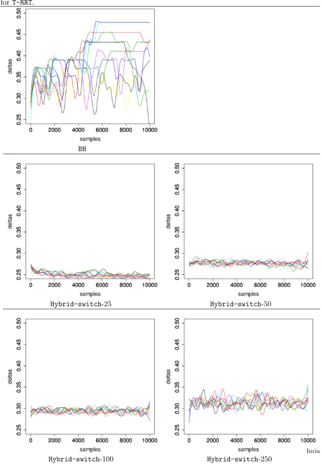
We next consider the variation of temperature. For Hybrid , after an initial delay period, the temperature appears to be a decreasing function of the switch parameter b. In particular, in Hybrid-switch-100 the temperature is almost the lowest (circa 1.5 unit) and is remarkably stable. In sharp contrast, BH progresses in stages to high temperatures. The propensity to remain for long periods in high energy regions is a consequence of temperature and step size adaptations, as larger temperatures are required to maintain a target acceptance ratio in such regions. More precisely, upon using a inadapted step size to extend a sample, the energy difference increases, lowering the acceptance rate. This in turns triggers a dramatic increase of the temperature (supp. Algorithms in Tables 1 and 2). Quenching occasionally manages to descend back to more moderate regions. However, in all cases, every cycle attains temperatures well beyond those observed for Hybrid . As for T-RRT, the temperature rises continuously, and reaches levels not seen for Hybrid nor for BH.

As for the stepsize, in the Hybrid algorithms, increasing values of b (increasing BH character) result in larger stepsizes. Hybrid-switch-100 does not quite reach the largest stepsize but again is stablest, staying within a narrow zone defined by 0.24 ≤ δ ≤ 0.27. For BH, stepsizes reach the largest values; they are also more variable compared to the other algorithms. We note that the stepsize is not varied in the T-RRT algorithm.

As a final analysis, we consider the correlation between the stepsize δ and the temperature, respectively initialized to δ = 0.2 and T = 2 (Fig. 10). For Hybrid , the temperatures explored are essentially symmetric with respect to the initial value, reflecting the adaptation to satisfy the target acceptance probability (supp. Table 1). For BH, while the range of delta explored is mildly broader (max value of 0.5 instead of 0.4), the temperature range for a given δ, on the other hand, is dramatically larger. This again reflects BH being trapped in regions with increasing energy, which requires raising the temperature to meet the target acceptance ratio.

4.5 Long run

Over the course of 120 hours, our long run of the Hybrid algorithm discovered 240,984 local minima, compared to 458,082 in BLN69-min-all. However, a total of 162,260 of the unique minima discovered have an energy below -100 units–as opposed to 5,932 in BLN69-min-E−100. We also note that all local minima in BLN69-min-top10 were discovered.

These results illustrate the ability of the algorithm to explore low-lying regions of the BLN69 landscape.

(14)

5 Discussion

This work introduces a novel global optimization algorithm, mixing two keys ingredients. The first is energy minimization as used by basin-hopping (BH), which allows identifying the basins visited in the course of a landscape exploration. The second is enhanced exploration of yet unexplored regions, resorting to the Voronoi bias rule, inherited from the (transition) rapidly growing random tree methods (T-RRT). In a nutshell, the algorithm Hybrid generates threads of local minima, each thread consisting of local minima generated by a contiguous sequence of extensions and quenches using BH, the first point of a thread being chosen with the Voronoi bias rule. The balance between BH and T-RRT extensions is a user defined parameter called the switch parameter, denoted b.

We focus on two aspects of the quality of the global optimization obtained using the T-RRT, BH, and Hybrid algorithms: the breadth of the exploration and the depth of the minima in terms of their potential energy. Generally speaking, while low-energy configurations can be discovered using BH and T-RRT–the latter upon quenching the conformations obtained. The

hybrid algorithm outperforms them in both respects. The Voronoi bias coupled with basin

hopping threads provides discovery and exploration of low-energy basins throughout the sampled

regions. The basin hopping algorithm clearly allows discovery of low-lying minima, but its

reliance solely on Monte Carlo moves to extend the current configuration can lead to periods in which the exploration remains in high-energy regions. As for T-RRT, while exploration is boosted by the Voronoi bias rule, the absence of quench allows only a slow return to low-energy regions, penalizing their exploration.

The breadth of exploration of the different algorithms reflects these observations. When con-sidering the entire set of discovered minima regardless of their energies, the size of the bounding box and RMSF of the sampled configurations is largest for BH and, to a lesser extent, T-RRT. However, these minima are principally associated with high-energy configurations. Focusing on the lower-energy configurations discovered by these two algorithms reveals that their diversity is much more limited than that of the configurations obtained by the hybrid Hybrid algorithm, especially with switch parameter b specifying a TRRT step every 50 or 100 basin-hopping steps. Practically, for the model protein used (BLN69), a value b ∼ 100 yields the best results both in terms of low energy minima discovered and breadth of exploration.

An important aspect of any Metropolis-based search algorithm is the choice of methods for choosing and/or adjusting the run parameters temperature and stepsize. Critically, in Hybrid the run parameter methods are reset upon starting each basin-hopping thread, which favors local adaptation to the region of the landscape being explored. In contrast, for BH, previous adjustments in the stepsize parameters tend to have too much influence on newly selected points, especially on terrains where there is a great variety of scales. In varied terrain T-RRT no doubt suffers from a fixed stepsize, although this may be an advantage for more thorough mapping of restricted regions. It may also be noticed that the Hybrid exploration results converge in a non-linear manner to those of BH as a function of increasing switch parameter b. This presumably is due to the algorithm failing to find a relevant stepsize when the switch parameter is small, as the reinitialization of parameters is performed too frequently.

Further exploration is called for, along several avenues. In all the Hybrid runs, the run parameters stabilized relatively early, suggesting that these parameters could be fixed at the stable values for subsequent runs, thus removing their interference with the attainment of detailed balance in the sampling. The dependence of the sampling on the progress variable (due to the T-RRT selection step) remains, however, but could possibly be taken into account so as to be able to compute equilibrium thermodynamics, in a spirit analogous to basin sampling. Given

(15)

the observed performance of Hybrid , an intriguing question is also to ascertain, under mild assumptions on the landscape and the switch parameter, the exhaustiveness of the exploration of low energy sub-level sets of the landscape. Finally, in terms of performance and the quality of the statstics obtained, it may be possible to include waste recycling strategies in order to make use of samples rejected at one stage of the exploration that may have relevance at later stages. Acknowledgments. The authors wish to thank D. Wales and M. Oakley for providing the database of stationary points of the BLN69 model. This work was financed in part by the CNRS

(16)

6 Artwork

Algorithm 1 Algorithm GenericPELSampler: a generic sampling algorithm for poten-tial energy landscapes.

Require: E(p): potential energy function of a given conformation p

Require: Parameters governing the exploration, typically the temperature T and the step size δ

Require: P : data structure hosting the conformations harvested Initialize the set P with one conformation

while StopCondition= False do

pn← SelectConfForExtension(P )

pe← Extend(pn)

if AcceptSample(pn, pe) then RecordNewSample(pe, P ) UpdateParams

Figure 1 The Hybrid algorithm Hybrid consists of interleaving calls to T-RRT and BH. In this cartoon, starting from the initial configuration (black dot), one step of T-RRT is performed after every three steps of BH (i.e., b = 3). The local minima generated by a contiguous sequence of BH extensions and quenches are represented with the same color. Each such set of local minima is also called a thread. Thus, in this example, Hybrid has generated four threads of size three.

(17)

Figure 2 Number of local minima discovered. Since for each algorithm ten runs were made, results are presented with boxplots. Note that for T-RRT, the samples generated were quenched so as to identify the basins visited.

● ● ● ● ● ● ● ● ● ● ● ● ● ● ● ● ● ● ● ● ● ● ● ● ● ● ● ● ● ● ● ● ● ● ● ● ● ● ● ● ● ● ● ● ● ● ● ● ● ● ● ● ● ● ● ● ● ● ● ● ● ● ● ● ● ● ● ● ● 2 4 6 8

trrt hyb−25 hyb−50 hyb−100 hyb−250 bh

Num. minima ● ● ● ● ● ● ● ● ● ● ● ● ● ● ● ● ● ● ● ● ● ● ● ● ● ● ● ● ● ● ● ● ● ● ● ● ● ● ● ● ● ● ● ● ● ● ● ● ● ● ● ● ● ● ● ● ● ● ● ● ● ● ● ● ● ● 0 100 200 300

Num. minima

Mins from BLN69-min-top10 Mins from BLN69-min-E−100

● ● ● ● ● ● ● ● ● ● ● ● ● ● ● ● ● ● ● ● ● ● ● ● ● ● ● ● ● ● ● ● ● ● ● ● ● ● ● ● ● ● ● ● ● ● ● ● ● ● ● ● ● ● ● ● ● ● ● ● ● ● ● ● 0 2000 4000

Num. no

v

el minima

(18)

Figure 3 Exploration breadth: statistics on the bounding boxes of the local minima from BLN 69 − min − all discovered.

● ● ● ● ● ● ● ● ● ● ● ● ● ● ● ● ● ● ● ● ● ● ● ● ● ● ● ● ● ● ● ● ● ● ● ● ● ● ● ● ● ● ● ● ● ● ● ● ● ● ● ● ● ● ● ● ● ● ● ● ● ● ● 5 10 15 20

BBo

x side: median length ●

● ● ● ● ● ● ● ● ● ● ● ● ● ● ● ● ● ● ● ● ● ● ● ● ● ● ● ● ● ● ● ● ● ● ● ● ● ● ● ● ● ● ● ● ● ● ● ● ● ● ● ● ● ● ● ● ● ● ● ● ● 50 100 150 200 250 300

BBo

x: diameter

Bounding box side (Bside) Bounding box diameter (Bdiam)

● ● ● ● ● ● ● ● ● ● ● ● ● ● ● ● ● ● ● ● ● ● ● ● ● ● ● ● ● ● ● ● ● ● ● ● ● ● ● ● ● ● ● ● ● ● ● ● ● ● ● ● ● ● ● ● ● ● ● ● ● ● 5 10 15 20

BBo x: v olume ● ● ● ● ● ● ● ● ● ● ● ● ● ● ● ● ● ● ● ● ● ● ● ● ● ● ● ● ● ● ● ● ● ● ● ● ● ● ● ● ● ● ● ● ● ● ● ● ● ● ● ● ● ● ● ● ● ● ● ● ● ● 2 3 4 5

Mean RMSF

(19)

Figure 4 Exploration breadth: statistics on the bounding boxes of the local minima

from BLN69-min-E−100 discovered.

● ● ● ● ● ● ● ● ● ● ● ● ● ● ● ● ● ● ● ● ● ● ● ● ● ● ● ● ● ● ● ● ● ● ● ● ● ● ● ● ● ● ● ● ● ● ● ● ● ● ● ● ● ● ● ● ● ● ● ● ● ● ● ● 0.0 2.5 5.0 7.5

BBo

x side: median length

● ● ● ● ● ● ● ● ● ● ● ● ● ● ● ● ● ● ● ● ● ● ● ● ● ● ● ● ● ● ● ● ● ● ● ● ● ● ● ● ● ● ● ● ● ● ● ● ● ● ● ● ● ● ● ● ● ● ● ● ● ● ● 0 25 50 75 100 125

BBo

x: diameter

Bounding box side (Bside) Bounding box diameter (Bdiam)

● ● ● ● ● ● ● ● ● ● ● ● ● ● ● ● ● ● ● ● ● ● ● ● ● ● ● ● ● ● ● ● ● ● ● ● ● ● ● ● ● ● ● ● ● ● ● ● ● ● ● ● ● ● ● ● ● ● ● ● ● ● ● ● ● 0 2 4 6

BBo x: v olume ● ● ● ● ● ● ● ● ● ● ● ● ● ● ● ● ● ● ● ● ● ● ● ● ● ● ● ● ● ● ● ● ● ● ● ● ● ● ● ● ● ● ● ● ● ● ● ● ● ● ● ● ● ● ● ● ● ● ● ● ● ● ● 0 1 2 3

Mean RMSF

(20)

Figure 5 Energies of the local minima from BLN 69 − min − all discovered. ● ● ● ● ● ● ● ● ● ● ● ● ● ● ● ● ● ● ● ● ● ● ● ● ● ● ● ● ● ● ● ● ● ● ● ● ● ● ● ● ● ● ● ● ● ● ● ● ● ● ● ● ● ● ● ● ● ● ● ● ● ● ● ● ● ● −100 −75 −50 −25 0

Mean energy ● ● ● ● ● ● ● ● ● ● ● ● ● ● ● ● ● ● ● ● ● ● ● ● ● ● ● ● ● ● ● ● ● ● ● ● ● ● ● ● ● ● ● ● ● ● ● ● ● ● ● ● ● ● ● ● ● ● ● ● ● ● ● ● −100 −75 −50 −25

Median energy

Mean energy (Emean) median energy (Emed.)

Figure 6 Run times in seconds of algorithms. NB: The run times for RRT include the quench of all conformations to identify the corresponding local minima.

● ● ● ● ● ● ● ● ● ● ● ● ● ● ● ● ● ● ● ● ● ● ● ● ● ● ● ● ● ● ● ● ● ● ● ● ● ● ● ● ● ● ● ● ● ● ● ● ● ● ● ● ● ● ● ● ● ● ● ● ● ● ● ● 10000 20000 30000

(21)

Figure 7 Evolution of energies during the runs of BH and Hybrid , as a function of the progress–number of conformations generated. Each plot features the ten runs of the algorithm scrutinized – one colored curve per algorithm. The curves were smoothed using a linear kernel with alpha parameter equal to 0.01.

BH T-RRT

Hybrid-switch-25 Hybrid-switch-50

(22)

Figure 8 Evolution of temperature T during the runs of BH and Hybrid , as a function of the progress–number of conformations generated.

BH T-RRT

(23)

Figure 9 Evolution of the step size δ during the runs of BH and Hybrid , as a function of the progress–number of conformations generated. Note that the step size δ is constant for T-RRT.

BH

(24)

Figure 10 Scatterplot of step size δ versus temperature T . One color corresponds to one run. 0.20 0.25 0.30 0.35 1.0 1.5 2.0 2.5 3.0 3.5 4.0 deltas temper atures 0.20 0.25 0.30 0.35 1.0 1.5 2.0 2.5 3.0 3.5 4.0 0.20 0.25 0.30 0.35 1.0 1.5 2.0 2.5 3.0 3.5 4.0 0.20 0.25 0.30 0.35 1.0 1.5 2.0 2.5 3.0 3.5 4.0 0.20 0.25 0.30 0.35 1.0 1.5 2.0 2.5 3.0 3.5 4.0 0.20 0.25 0.30 0.35 1.0 1.5 2.0 2.5 3.0 3.5 4.0 0.20 0.25 0.30 0.35 1.0 1.5 2.0 2.5 3.0 3.5 4.0 0.20 0.25 0.30 0.35 1.0 1.5 2.0 2.5 3.0 3.5 4.0 0.20 0.25 0.30 0.35 1.0 1.5 2.0 2.5 3.0 3.5 4.0 0.20 0.25 0.30 0.35 1.0 1.5 2.0 2.5 3.0 3.5 4.0 0.15 0.20 0.25 0.30 0.35 0.40 0.45 0 50 100 150 200 deltas temper atures 0.15 0.20 0.25 0.30 0.35 0.40 0.45 0 50 100 150 200 0.15 0.20 0.25 0.30 0.35 0.40 0.45 0 50 100 150 200 0.15 0.20 0.25 0.30 0.35 0.40 0.45 0 50 100 150 200 0.15 0.20 0.25 0.30 0.35 0.40 0.45 0 50 100 150 200 0.15 0.20 0.25 0.30 0.35 0.40 0.45 0 50 100 150 200 0.15 0.20 0.25 0.30 0.35 0.40 0.45 0 50 100 150 200 0.15 0.20 0.25 0.30 0.35 0.40 0.45 0 50 100 150 200 0.15 0.20 0.25 0.30 0.35 0.40 0.45 0 50 100 150 200 0.15 0.20 0.25 0.30 0.35 0.40 0.45 0 50 100 150 200 0.15 0.20 0.25 0.30 0.35 0.40 0.45 0 50 100 150 200 0.15 0.20 0.25 0.30 0.35 0.40 0.45 0 50 100 150 200 Hybrid-switch-100 BH

References

[1] Y. Sugita and Y. Okamoto. Replica-exchange molecular dynamics method for protein fold-ing. Chemical physics letters, 314(1):141–¡151, 1999.

[2] A. Mitsutake and Y. Okamoto. Multidimensional generalized-ensemble algorithms for com-plex systems. J Chem Phys, 130(21):214105, Jun 2009.

[3] A.P. Lyubartsev, A.A. Martsinovski, S.V. Shevkunov, and P.N. Vorontsov-Velyaminov. New approach to Monte Carlo calculation of the free energy: Method of expanded ensembles. J. Chem. Phys, 96:1776–83, 1992.

[4] S. Kirkpatrick and M-P. Vecchi. Optimization by simmulated annealing. science,

220(4598):671–680, 1983.

[5] Z. Li and H.A. Scheraga. Monte carlo-minimization approach to the multiple-minima prob-lem in protein folding. PNAS, 84(19):6611–6615, 1987.

[6] Michael C Prentiss, David J Wales, and Peter G Wolynes. Protein structure prediction using basin-hopping. The Journal of Chemical Physics, 128(22):225106, 2008.

[7] R. Elber and M. Karplus. Multiple conformational states of proteins: a molecular dynamics analysis of myoglobin. Science, 235(4786):318–321, 1987.

[8] J.M. Troyer and F.E. Cohen Becker. Protein conformational landscapes: Energy minimiza-tion and clustering of a long molecular dynamics trajectory. Proteins: Structure, Funcminimiza-tion, and Bioinformatics, 23(1):97–110, 1995.

[9] M. Wevers, J.C. Sch¨on, and M.Jansen. Global aspects of the energy landscape of metastable

crystal structures in ionic compounds. Journal of Physics: Condensed Matter, 11(33):6487, 1999.

(25)

[10] Fugao Wang and DP Landau. Efficient, multiple-range random walk algorithm to calculate the density of states. Physical review letters, 86(10):2050, 2001.

[11] A. Laio and M. Parrinello. Escaping free-energy minima. PNAS, 99(20):12562–12566, 2002.

[12] L. Jaillet, F.J. Corcho, J-J. P´erez, and J. Cort´es. Randomized tree construction algorithm

to explore energy landscapes. Journal of computational chemistry, 32(16):3464–3474, 2011. [13] Michael C Prentiss, David J Wales, and Peter G Wolynes. The energy landscape, folding pathways and the kinetics of a knotted protein. PLoS computational biology, 6(7):e1000835, 2010.

[14] Graeme G. Henkelman, G. J´ohannesson, and H. J´onsson. Methods for finding saddle points

and minimum energy paths. In Theoretical Methods in Condensed Phase Chemistry, pages 269–302. Springer, 2002.

[15] D.J. Wales. Discrete path sampling. Molecular Physics, 100(20):3285–3305, 2002. [16] D.J. Wales. Energy Landscapes. Cambridge University Press, 2003.

[17] Steven M LaValle and James J Kuffner Jr. Rapidly-exploring random trees: Progress and prospects. In B.R. Donald, K.M. Lynch, and D. Rus, editors, Algorithmic and Computational Robotics: New Directions, pages 293–308. A K Peters, 2001.

[18] James J Kuffner and Steven M LaValle. Rrt-connect: An efficient approach to

single-query path planning. In Robotics and Automation, 2000. Proceedings. ICRA’00. IEEE

International Conference on, volume 2, pages 995–1001. IEEE, 2000.

[19] H. Samet. Foundations of multidimensional and metric data structures. Morgan Kaufmann, 2006.

[20] Peter N Yianilos. Data structures and algorithms for nearest neighbor search in general metric spaces. In ACM SODA, volume 93, pages 311–321, 1993.

[21] S. O’Hara and B.A. Draper. Are you using the right approximate nearest neighbor algo-rithm? In Applications of Computer Vision (WACV), 2013 IEEE Workshop on, pages 9–14. IEEE, 2013.

[22] Didier Devaurs, Thierry Sim´eon, and Jorge Cortes. Enhancing the transition-based rrt to

deal with complex cost spaces. In Robotics and Automation (ICRA), 2013 IEEE Interna-tional Conference on, pages 4120–4125. IEEE, 2013.

[23] Scott Brown, Nicolas J. Fawzi, and Teresa Head-Gordon. Coarse-grained sequences for protein folding and design. Proc Natl Acad Sci U S A, 100(19):10712–10717, Sep 2003. [24] M. T. Oakley, D. J. Wales, and R. L Johnston. Energy landscape and global optimization

for a frustrated model protein. The Journal of Physical Chemistry B, 115(39):11525–11529, 2011.

[25] F. Cazals, T. Dreyfus, D. Mazauric, A. Roth, and C.H. Robert. Conformational ensem-bles and sampled energy landscapes: Analysis and comparison. Journal of Computational Chemistry, NA(in press), 2015.

(26)

Table 1 Temperature adaptation (left) BH and Hybrid (right) T-RRT.. The temperature T is adapted in BH and Hybrid as to tend towards a target probability, representing the fraction of accepted samples desired, whilst in T-RRT by taking into consideration the maximal energy variation of the present conformational ensemble.

Require: current proba: fraction of so far ac-cepted points

target proba: desired value for

current proba

nb accepts: number of accepted points

nb attempts: number of attempts for the

if nb attempts%nb temp check == 0 then current proba ← nb accepts/nb attempts if current proba > target proba then

T ← T ∗ λ else

T ← T /λ

Require: Enew: energy of the point to be in-serted

Eold: energy of the currently processed point

lambda: preset parameter

C: the current conformational ensemble energyRange: the current maximal energy variation of the conformational ensemble

if Enew> Eold then

if pnewisaccepted then

T ← T /2(Enew−Eold)/0.1∗energyRange(C)

else

T ← T ∗ 2λ

(27)

Algorithm 2 Stepsize adaptation BH and Hybrid . The stepsize δ is adapted in the same manner as to tend to a target probability, representing the fraction of extended samples that belong to a different basin.

Require: current proba: fraction of extended points outside the current basin target proba: desired value for current proba

nb basin exit: number of extensions outside the current basin nb attempts: number of attempts for the previous

nb delta check: frequency at which the condition on target proba is checked

{target proba}

if nb attempts%nb delta check == 0 then current proba ← nb basin exit/nb attempts; if current proba < target proba then

δ ← δ ∗ τ else

δ ← δ/τ

Figure 11 2D sketch of the energy landscape representing BLN69-top10 using multi dimensional scaling (MDS) on a matrix of pairwise cumulative distances. The distance used is the least root mean deviation (lRMSD ). The Fig. is reproduced from [25] for convenience.