HAL Id: hal-03189300
https://hal-amu.archives-ouvertes.fr/hal-03189300
Submitted on 3 Apr 2021
HAL is a multi-disciplinary open access
archive for the deposit and dissemination of
sci-entific research documents, whether they are
pub-lished or not. The documents may come from
teaching and research institutions in France or
abroad, or from public or private research centers.
L’archive ouverte pluridisciplinaire HAL, est
destinée au dépôt et à la diffusion de documents
scientifiques de niveau recherche, publiés ou non,
émanant des établissements d’enseignement et de
recherche français ou étrangers, des laboratoires
publics ou privés.
Maxime Chiletti, Jean-Luc Duchateau, Frédéric Topin, Bernard Turck, Louis
Zani
To cite this version:
Maxime Chiletti, Jean-Luc Duchateau, Frédéric Topin, Bernard Turck, Louis Zani.
ASC2018-3LPo2A-03. IEEE Transactions on Applied Superconductivity, Institute of Electrical and Electronics Engineers,
2020. �hal-03189300�
Abstract — In spite of their complex geometry, CICCs have to be modelled with a rather simple description for coupling losses when operating in transient regime. Difficulties to predict AC losses in superconducting cable have already been shown in previous models such as the new analytical one developed at CEA named COLISEUM (after COupling Losses analytIcal Staged cablEs Unified Model) and CEA heuristic one MPAS. In this paper, we present a parametric analysis for coupling losses in superconducting strands and cables subjected to time-varying transverse magnetic field by using the recently developed COLISEUM. This analysis aims at understanding trends of the model in a broad domain of investigation and their associated limits of application. We show that for a wide range of parameters, it is possible to reduce this model of four time constants to a smaller subset. This reduction brings simplifications to the current COLISEUM and enables it to be consistent with the number of time constants considered in the MPAS model from CEA.
Index Terms—AC losses, superconducting, CICCs, stability
I. INTRODUCTION
Estimating AC losses in CICCs made of numerous superconducting strands has been approached along different methods [1]-[2]. Those methods privilege numerical calculations of all interactions between every strand. At CEA, our approach aims at a more global analysis. After experimental observations of AC losses vs frequency, it has been shown that a CICC can be characterized by a set of well identified time constants. This led us to the MPAS model [3].This model firstly used for JT60SA conductor is now well used to analyze AC losses in cables, in particular all those of the ITER magnets [4].
In this line, CEA has developed a new theoretical model based on analytical calculations of the interactions between stages of a cable [5]-[8]. That code “COLISEUM’’ has the purpose to support the code MPAS and make it evolve as the theory progresses. In this paper, detailed results of calculations with COLISEUM with a two stage cables are depicted. Parameters have been varied over wide ranges. The strong link between twist pitches 𝑙𝑝 and transverse conductance 𝜎 is discussed. It
is shown also that among the 4 time constants 𝜏𝑗 obtained by the calculation, a system with only two time constants is amply sufficient for the evaluation of AC losses over a large range of frequencies. We also focus for the first time on how real composite strands can interact between themselves, exploring the fundamental case of a triplet of composites.
This reduction to two time constants could also be a first step for model enhancement to a three stages cable description and behavior comparison with MPAS.
Manuscript submitted for review 26 October 2018. This work was supported in part by ASSYSTEM.
M. Chiletti (corresponding author phone: +33442254749; e-mail:
[email protected]), L. Zani, B. Turck and JL. Duchateau are with Commissariat à l’Energie Atomique et aux Energies Alternatives, CEA/DRF/IRFM, CEA Cadarache 13108 St Paul-Lez-Durance, France. M.Chiletti is also with Aix Marseille Université, CNRS, IUSTI UMR 7343, 13453, Marseille, France together with F. Topin.
II. SUMMARY OF PREVIOUS WORKS AND PRESENTATION OF THE METHOD
In the work presented below, the method is explained in detail for the case of the first stage of many CICC cables, i.e. triplet of superconducting composite. The composite itself has a specific behavior, as it results of the aggregation of the SC filaments in many concentric layers. The magnetic interaction of 3 composites cabled in a triplet is not solvable right away. Some preliminary work has to be done to transform the basic composite in an equivalent one stage composed of N superconducting tubes (N-uplet), placed as a corona. Then it is possible, thanks to the code COLISEUM to estimate losses in a two stage cable N1 × N2.
In a multi-filamentary composite such as the one seen in figure 1 and described in [7], volumetric dissipated power can be written 𝑃𝑣𝑜𝑙 = ∑ 𝑛𝜏𝑖𝐵𝑖
̇2 𝜇0 2
𝑖=1 . The sum over two terms comes from
the number of interfaces between superconducting material and non-superconducting ones inside the composite. Actually in our present case, as the resistivity in the filamentary zone and the copper are similar only one time constant does exist. The multistage cable, with two stages N1 and N2 has been studied in detail. It has been shown that for a sinusoidal field variation, coupling losses per cycle 𝑄(𝜔) can be written as:
𝑄(𝜔) =𝐵𝑝 2𝜋𝜔 𝜇0 ∑ 𝑛𝜅𝑗𝜏𝑗 1+(𝜔𝜏𝑗)2 4 𝑗=1 (1)
III. MODELLNG A SC COMPOSITE
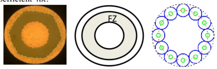
The composite is replaced by a N-uplet of superconducting tubes of radius 𝑅𝑓 (green circle in figure 1) placed on a circle.
The conductance 𝜎 between those tube strands is estimated in order to get the real time constant of the composite. The radius 𝑅𝑓 has been adjusted to obtain the same shielding
coefficient 𝑛𝜅.
Fig. 1. JT-60SA TF strand on the left, its simplified scheme in the middle and its N-uplet formulation on the right. Each blue circle represents an element of radius 𝑹𝟏 in the N-uplet. Cabling radius 𝑹𝒄 is the red dashed line (right
shceme) gathering gravity centre of each element. TABLE I MAIN PARAMETERS
Geometrical characteristics, time constant and shielding coefficient of the reproduced strand using the N-uplet model (third scheme on the right).
Geometrical parameters of filaments in the N-uplet model are chosen to perfectly reproduce the real strands behavior (twist pitch 𝑙𝑝, radii 𝑅1, 𝑅𝑓 and 𝑅𝑐, conductance 𝜎 …).
Analytical Modelling of CICCs Coupling Losses:
Broad Investigation of Two-Stage Model.
M. Chiletti, J.L. Duchateau, F. Topin, B. Turck, L. Zani.
N 𝑙𝑝1 (mm) 𝑅𝑐1 (mm) 𝑅1 (mm) 𝑅𝑓 𝑅1 ⁄ (S.m-1) 12 15 0.3217 0.0833 0.3 9.9e9 ms) n 18.36 1.247
FZ
1 𝜏 𝜏( Ω2 → ∞ ) Ω1 Ω2 0 Bundle of radius 𝑅𝑐1+ 𝑅1 Cabling radius 𝑅𝑐2 Cabling radius 𝑅𝑐1
This new ‘composite strand' will tend to be a first step to the insertion of the composite in the two stage model. Many tubes of radius 𝑅1 placed as a corona can reproduce the shielding and
the magnetic behavior of the real strand itself. This hypothesis was tested with several corona composed of a different number of strands (8, 12, 24). Given a lineic conductance between elements in the N-uplet, we can reproduce the behavior of the real JT-60SA-TF strand giving the same time constant and shielding coefficient. Let’s note that the circumscribed areas, of the real strand (JT-60SA) and of the corona used to reproduce it, are the same. Elements radii in the corona are chosen to fit this requirement (see table I). The reproduction of the magnetic behavior of the strand with a one stage model is mandatory in order to include this fundamental stage (strand) in the existing two stage model.
IV. FIRST STAGE OF CABLED STRANDS For a given value of conductance between the elements of the second stage (𝜎𝑠𝑢𝑝𝑒𝑟𝑠𝑡𝑎𝑔𝑒 or 𝜎2), of 5𝑒7 𝑆. 𝑚−1, the results
with time constants and shielding coefficient are depicted in Table II. That value of conductance is taken at that level to better illustrate the coupling effects between the three composites. As already stated, our two stage model leads to four time constant system. First stage geometrical parameters of this cable are taken from Table I, and second stage parameters are deduced from tangency condition in a triplet plus using the twist pitch of the first stage of JT-60SA-TF cable with 𝑙𝑝2= 45 𝑚𝑚.
Fig. 2. A triplet of strands in a two-stage approach. Table II COLISEUM OUTPUTS
Time constants and shielding coefficient of the system depicted in Fig. 2 calculated by COLISEUM.
From here, shielding coefficient (n) will be referred to the circumscribed area of the circumscribed cable. As we can see in the above table, 𝜏 and 𝑛𝜅 of the strand (N°2) are still present in the system but slightly modified. The strand shielding coefficient of 0.84 seems different from the one found with the strand model alone but this is only due to reference area. Once reported to the circumscribed area of one element only (corona of 12 strands), we obtain:
𝑛𝜅2𝑐𝑖𝑟𝑐𝑢𝑚= 0.84 × 1.55 = 1.3 .
This is in agreement with the shielding coefficient found in the strand model and in the N-uplet description.
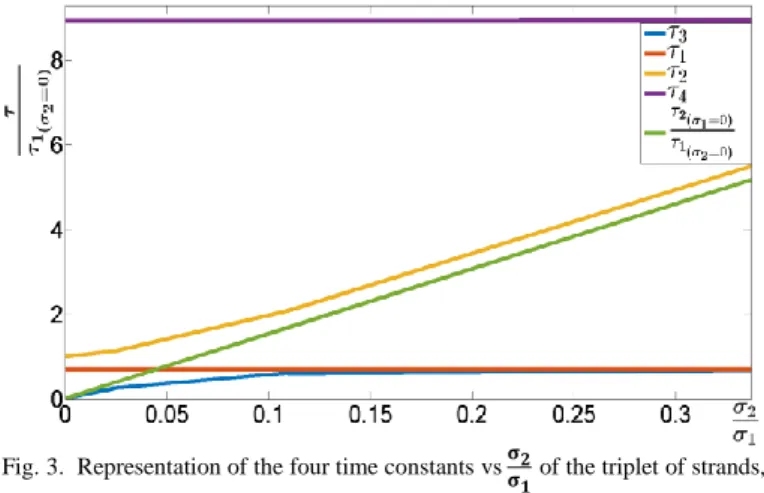
In a first step, keeping constant the twist pitches lengths, the conductance of the second stage has been varied. The results are shown in figure 3. It can be seen in figure 3 below that among the four time constants given by COLISEUM only two do vary with the ratio 𝜎2
𝜎1, 𝜏2 and 𝜏3, the two others 𝜏1 and 𝜏4 are
constant. But, for these time constants, shielding coefficients are less than 10−3 as seen for the whole range in the example
of table II. That leads us to validate a way to reduce to a two time constant system.
Fig. 3. Representation of the four time constants vs 𝛔𝟐
𝛔𝟏of the triplet of strands, obtained through COLISEUM.
In order to get a quick insight into a two-stage system, some simple calculation can be also done on a 2x2 cable which can be analytically solved. Considering a system where 2 𝑙𝑝1= 𝑙𝑝2, with only magnetic coupling between two current loops and currents flowing in elements with no mixing. These two independent current loops, representing the two stages are characterized by their inductances (𝐿1, 𝐿2, 𝑀12) and two
electrical resistances (Ω1 and Ω2). The solutions of the two
associated differential equations identify two time constants 𝜏±:
𝜏±= 6𝐿1
(4Ω1+Ω2)∓√16Ω12−4Ω1Ω2+Ω22
(2)
Represented in figure 3, we can see the limits and asymptotical behavior of this simple two-stage model.
Fig. 4. Representation of the two time constants given by the expression (2).
In this analytical description, when one sub-system decouples (one of the two sigma goes to 0), the global system is led by only one time constant. Indeed, on one side (left of the graph) only one time constant survives whereas on the other side both survive but one of the two is killed by its very low shielding coefficient.
V. TIME CONSTANT NUMBERS REDUCTION If the contact between first and second stage is cut (𝜎2= 0),
then, the remaining time constant is the one linked to the substage and the three other ones are killed by their very low
N° ms) n
1 12.73 5.2e-4
2 18.789 0.84
3 1.047 0.316
4 0.5 1 2 3 4 5 6 0.5 6 0.5 6 4 1 4 1 4 1 3 2
shielding coefficient (inferior to 10−4). In fact, when 𝜎2= 0,
the three bundles representing strands are electrically independent and it is as if we would have three individual strands without interaction. Only the strand time constant is non-zero. Whereas when the contact between elements in the first stage is cut (𝜎1= 0) the remaining time constant is the
one linked to the strand triplet (super-stage) and the three other constants killed themselves by falling to 0. When 𝜎1= 0,
contacts between first stage elements are destroyed and only the magnetic coupling between them is expressed. The behavior of the model seems to be in perfect agreement with what’s expected and given by the little analytical doublet of doublets. In the case of the triplet of composites, the two time constants we are dealing with are respectively 𝜏𝜎2=0= 18.3 𝑚𝑠
and 𝜏𝜎1=0= 1.45 𝑚𝑠 which are slightly different from the ones
we initially found. These two constants found at the limit of the model are supposed to be the proper time constants of each stage (sub and super) supposed isolated and without interaction. The three models (strands, one stage and two stage cable) are consistent with each other’s and give the same results.
We have made a broad investigation of the model (time constants, shielding coefficients) for different twist pitches ratios and conductances ratios. These two parameters were chosen because of their relevance as given in expression (2) to the application of the MPAS model. So it was obvious to check the variation of our model with respect to these two parameters contained in the computation of 𝑛𝜅 and 𝜏. Broad cartographies are established to identify the number (indicated inside colored domains) of couples ( 𝜏, 𝑛𝜅) contributing to the computation of AC losses up to defined contribution percentages (on the right of Fig. 5).
Fig. 5. Cartographic inventory of most contributing 𝒏𝜿𝒊𝝉𝒊.
We have considered a wide investigation over the spectrum of frequencies. The results are quite general. An example is given of the results for the low frequencies regime. In this case, the sum ∑𝑖𝑛𝜅𝑖𝜏𝑖 is representative of the losses. Figure 5 represents
the zone where one to four time constants contribute to the
losses for a product 𝑛𝜅𝑖𝜏𝑖 larger than a given percentage of the
total ∑ 𝑛𝜅𝑖 𝑖𝜏𝑖. As visible in Figure 5, this two-stage model can
be reduced to two time constants (blue region) in a realistic domain of application regarding the twist pitches ratio (around 2) and conductances ratio.
VI. ROLE OF THE CONDUCTANCES
Using different approaches to compute losses (low frequency formulation and COLISEUM [7]), we have noticed that it exists a relation of equality between n sums, and thus on losses in low frequencies, for the same geometrical configuration but with different electrical boundary condition. 𝑛𝜅2𝜏2+ 𝑛𝜅3𝜏3= 𝑛𝜅′1𝜏𝜎2=0+ 𝑛𝜅′2𝜏𝜎1=0= 𝑛𝜅𝜏𝑠𝑢𝑏+ 𝑛𝜅𝜏𝑠𝑢𝑝
① ② ③ In the first brace are gathered, 𝜏2 and 𝜏3 with their respective
shielding coefficient 𝑛𝜅2 and 𝑛𝜅3 (given in Table II and figure
3), the output of COLISEUM with complete coupling between stages.
The second brace refers to the combination of two cases: the sum of 𝑛𝜅𝑖 and 𝜏𝑖 obtained for either 𝜎1= 0, or 𝜎2= 0. That is
the sum of proper behavior of each of the two stages independently. The third one, substage and super-stage contribution to AC losses are depicted using the low frequency approach for a two stage cable (see [7]). Application concerning the triplet of composite is given in Table III below.
TABLE III
EVALUATION OF THE TRIPLE EQUALITY
Geometrical parameters are those corresponding to figure 2. L means left part of a brace and R means right part.
This triple equality well reflects the MPAS philosophy where one time constant belongs to each stage before coupling to the next stage. 𝑛𝜅 𝟎. 𝟗𝟑 (a) 𝟎. 𝟖𝟏 𝟎. 𝟖𝟒 𝟎. 𝟑𝟐 𝜏3 𝜏𝜎1=0 𝜏𝜎2=0 𝜏2 𝜏 (𝑚𝑠) (𝟏. 𝟎𝟓) (𝟏. 𝟒𝟐) (𝟏𝟖. 𝟑) (𝟏𝟖. 𝟕𝟗) 𝒏𝜿 𝟏. 𝟏𝟑 (b) 𝟎. 𝟗𝟑 𝟎. 𝟖𝟏 𝟎. 𝟎𝟑𝟑 𝜏3 𝜏𝜎1=0 𝜏𝜎2=0 𝜏2 𝜏 (𝑚𝑠) (𝟕. 𝟗𝟔) (𝟏𝟒. 𝟐𝟔)
(𝟏𝟖. 𝟑) (𝟐𝟒. 𝟕) Fig. 6. Set of time constants and shielding coefficients for a triplet of composites for two different transverse conductances.
N° (ms) 𝜏L nL 𝑛𝜅𝜏 L (ms) (ms) 𝜏R nR 𝑛𝜅𝜏 R (ms) Σ (ms) ① ② 18.79 18.3 0.84 0.81 15.8 14.8 1.05 1.43 0.32 0.93 0.34 1.34 16.12 16.12 ③ 14.8 1.33 16.12 𝜎2 𝜎1 1 1% 5% 10% 𝑙𝑝2 𝑙𝑝1 1 1 2 3 2 2 2 2 2 2 2 3
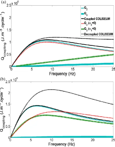
In figure 6, are represented in a diagram with 𝑛𝜅 and 𝜏, values obtained for the triplet of composite. The upper part is with 𝜎2= 5𝑒7 𝑆. 𝑚−1, and is the one discussed in section IV.
The red and green lines are either for 𝜎1= 0 or 𝜎2= 0, as explained above. The blue ones are for the coupled system through complete calculation. The lower part (b) shows the same results for a 10 times higher conductances 𝜎2=
5𝑒8 𝑆. 𝑚−1. Along this exploration of COLISEUM, we have
reached the fact that conductances (as interpreted in COLISEUM, i.e. conductances between stages) are as important as twist pitches ratio in time constants and losses computation. In fact, we have also verified that conductances and (twist pitches lengths) are permutable in time constants or losses computation.
VII. AN APPLICATION OVER THE RANGE OF FREQUENCIES
Using the n𝜅 and 𝜏 value given in figure 6, AC losses vs frequency have been computed. The influence of each stage to total losses highly depends on the conductance attributed to this stage. Using expression (1), we obtain the curves given in figure 7 below:
(a)
(b)
Fig. 7. AC losses 𝑸 vs frequency, for the cases depicted in figure 6. Ordinate axis range is conserved to show the curves deformation between cases (a) and (b).
Curves (a) top and (b) bottom in figure 7 are drawn using values and color codes from cases (a) and (b) of figure 6. Fully coupled and decoupled approaches are matching in the low frequency range as assessed by the previous triple equality. Continuous blue and black curves depict AC losses for the fully coupled system whereas dotted black, red and green curves are used for decoupled system as explained earlier. In the top curves (a) it is seen that when two basic time constants
are well separated, the 𝑄 vs 𝑓 curves slightly differ in the usual range of frequencies (less than 10 Hz). On the other hand when they come closer (bottom curves (b)), in the decoupled system the result is an accumulation of the amplitudes, while the coupled system leads to the emergence of a larger time constant. This results in different maximums although the initial slopes are equal.
Based on those theoretical results the MPAS model will be modified and enhanced step by step to better take into account conductances and coupling effect between stages.
VIII. CONCLUSION
The recently developed COLISEUM had shown its capability to simulate multiplets of composites starting from strands level. Based on the idea that a strand shields its enclosed volume using its exterior edge filaments, we use the one stage COLISEUM to reproduce strands behavior using a corona where basics elements are superconducting tubes used as filaments. Thus multiplets of composites can be simulated using the two stages COLISEUM to better understand interactions at a basic level of a CICC’s. Modelling the same system with different models (CLASS [8]or COLISEUM) we are able to get consistent results concerning the magnetic behavior of the system regarding time constant, shielding coefficient and thus losses.
It has been shown that COLISEUM which had initially four time constant can be reduced to two time constants in a wide range of frequencies and be consistent with the MPAS description of losses using one time constant per stage. Once geometrical parameters have been chosen, only transverse conductances between stages can be tested as free parameters until measurements will determine it. The relevance of conductances ratio has been highlighted through a broad investigation with the COLISEUM. This enhancement by COLISEUM could be a useful tool to guide MPAS in the experimental data fittings.
Thus, confronting MPAS and COLISEUM on experimental data such as the JT-60SA TF conductor will be the next step of our work to see to what extend COLISEUM could drive MPAS fit and improve MPAS description of CICC’s.
At higher frequencies, losses cannot be calculated using only sum of 𝑛𝜅𝜏’s as in cartographies of the figure 5. These studies are meant to be reproduced at higher frequency looking at each time constant contribution to the total losses in order to see whether the two time constant reduction is persistent with increasing frequencies. Same results as at low frequency are expected.
Concerning the low frequencies, the triple equality enlightens us. We could think that coupling effect between stages is weak. In fact it has no effect on the total calculated losses but plays a role in the contributions from each stage to these same losses. It could be therefore interesting to explore the role of the conductance ratio more in details as it reflects the different compaction stage for a same cable. Experimental campaign of AC losses measurement on different compaction levels are in progress on JT-60TF conductor. Data will be fitted using MPAS and COLISEUM.
AKNOWLEGMENT
Authors would like to thank S. Constans and Y. Stefan from ASSYSTEM for their financial and technical support leading to the realization of the work presented here.
REFERENCES
[1] Van Lanen, E. P. A. & Nijhuis, A. ‘‘JackPot: A novel model to study the influence of current non-uniformity and cabling patterns in cable-in-conduit conductors.’’ Cryogenics, vol. 50, Mar 2010.
[2] M. Breschi, P.L. Ribani, ‘‘Electromagnetic Modelling of the Jacket in Cable-in-Conduit Conductors.’’ IEEE Trans. On App. Sup., vol. 18, NO. 1, March 2008
[3] B. Turck, L. Zani, “A macroscopic model for coupling current losses in cables made of multi-stages of superconducting strands and its experimental validation.” Cryogenics, vol. 50, pp. 443-449, Aug 2010.
[4] D. Bessette “Design of a Nb3Sn Cable in Conduit Conductor to withstand the 60000 electromagnetic cycles of the ITER central solenoid” IEEE Trans. On App. Sup., vol.24, USA, Sept. 2013.
[5] A. Louzguiti, “AC coupling losses in CICCs: analytical modeling and experimental results on ITER CS conductor.” IEEE Trans. On App. Sup., vol. 27, Jun. 2016.
[6] A. Louzguiti, “Development of a new generic analytical modeling of AC coupling losses in cable-in-conduit conductors.” IEEE Trans. On App. Sup., vol. 28, Apr. 2018.
[7] A. Louzguiti, “Magnetic screening currents and coupling losses induced in superconducting magnets for thermonuclear fusion”, PhD thesis France, CEA, Dec. 2017.
[8] A. Louzguiti, L. Zani, D. Ciazynski, B. Turck, and F. Topin, “Development of an analytical-oriented extensive model for AC coupling losses in multilayer superconducting composite,” IEEE Trans. On App. Sup., vol. 26, Apr. 2016.