HAL Id: hal-02929450
https://hal.archives-ouvertes.fr/hal-02929450
Submitted on 27 Oct 2020
HAL is a multi-disciplinary open access
archive for the deposit and dissemination of
sci-entific research documents, whether they are
pub-lished or not. The documents may come from
teaching and research institutions in France or
abroad, or from public or private research centers.
L’archive ouverte pluridisciplinaire HAL, est
destinée au dépôt et à la diffusion de documents
scientifiques de niveau recherche, publiés ou non,
émanant des établissements d’enseignement et de
recherche français ou étrangers, des laboratoires
publics ou privés.
observations and a land surface model
K. Rebel, R. de Jeu, P. Ciais, N. Viovy, S. Piao, G. Kiely, A. Dolman
To cite this version:
K. Rebel, R. de Jeu, P. Ciais, N. Viovy, S. Piao, et al.. A global analysis of soil moisture derived from
satellite observations and a land surface model. Hydrology and Earth System Sciences, European
Geosciences Union, 2012, 16 (3), pp.833-847. �10.5194/hess-16-833-2012�. �hal-02929450�
www.hydrol-earth-syst-sci.net/16/833/2012/ doi:10.5194/hess-16-833-2012
© Author(s) 2012. CC Attribution 3.0 License.
Earth System
Sciences
A global analysis of soil moisture derived from satellite observations
and a land surface model
K. T. Rebel1,2, R. A. M. de Jeu2, P. Ciais3, N. Viovy3, S. L. Piao3, G. Kiely4, and A. J. Dolman2
1Department of Environmental Sciences, Copernicus Institute of Sustainable Development, Utrecht University,
Utrecht, The Netherlands
2Department of Earth Sciences, Faculty of Earth and Life Sciences, Vrije Universiteit Amsterdam,
Amsterdam, The Netherlands
3Laboratory for Climate Sciences and the Environment (LSCE), CEA-CNRS-UVSQ, Gif-sur-Yvette, France 4Department of Civil & Environmental Engineering, Centre for Hydrology, Micrometeorology and Climate Change,
University College Cork, College Road, Cork, Ireland
Correspondence to: K. T. Rebel (k.t.rebel@uu.nl)
Received: 26 March 2011 – Published in Hydrol. Earth Syst. Sci. Discuss.: 29 April 2011 Revised: 6 January 2012 – Accepted: 17 February 2012 – Published: 16 March 2012
Abstract. Soil moisture availability is important in
regulat-ing photosynthesis and controllregulat-ing land surface-climate feed-backs at both the local and global scale. Recently, global remote-sensing datasets for soil moisture have become avail-able. In this paper we assess the possibility of using re-motely sensed soil moisture – AMSR-E (LPRM) – to sim-ilate soil moisture dynamics of the process-based vegeta-tion model ORCHIDEE by evaluating the correspondence between these two products using both correlation and au-tocorrelation analyses. We find that the soil moisture prod-uct of AMSR-E (LPRM) and the simulated soil moisture in ORCHIDEE correlate well in space and time, in particular when considering the root zone soil moisture of ORCHIDEE. However, the root zone soil moisture in ORCHIDEE has on average a higher temporal autocorrelation relative to AMSR-E (LPRM) and in situ measurements. This may be due to the different vertical depth of the two products – AMSR-E (LPRM) at the 2–5 cm surface depth and ORCHIDEE at the root zone (max. 2 m) depth – to uncertainty in precipitation forcing in ORCHIDEE, and to the fact that the structure of ORCHIDEE consists of a single-layer deep soil, which does not allow simulation of the proper cascade of time scales that characterize soil drying after each rain event. We conclude that assimilating soil moisture, using AMSR-E (LPRM) in a land surface model like ORCHIDEE with an improved hy-drological model of more than one soil layer, may signifi-cantly improve the soil moisture dynamics, which could lead to improved CO2and energy flux predictions.
1 Introduction
Changes in land CO2 uptake and emissions at mid
lati-tudes are strongly related to the frequency and magnitude of droughts (Angert et al., 2005) and are, thus, ultimately linked to variations and possible future changes in the global hydrological and carbon cycles. Details of when, where, and how strong this coupling is, are largely unknown. Summer droughts under future climate conditions are likely to in-crease in frequency and intensity over Europe (Seneviratne at al., 2006b), parts of Northern America and the Mediter-ranean area according to the IPCC (Solomon et al., 2007), but there is doubt as to whether this is already visible in the observational record (van der Schrier, 2006). Various regions in the world also appear more sensitive to regional and local scale atmospheric feedbacks induced by soil moisture status that can increase the persistence and likelihood of drought (e.g. Koster et al., 2004; Seneviratne et al., 2006a). Albert-son et al. (2001) and D’Andrea et al. (2006) even suggest that wet and dry summers may exhibit bimodal distributions of soil moisture. This implies that changes from relatively wet- and carbon fixating conditions- towards dry- and carbon emitting-conditions, may be far more abrupt than previously thought.
Angert et al. (2005) suggest that hydrological processes, such as soil moisture availability, may in fact be more impor-tant in the carbon uptake of vegetation than the traditionally studied growth enhancing temperature effects (see also Ciais et al., 2005; Reichstein et al., 2007). Recent land-surface
modelling intercomparisons point to the need to focus on an accurate description of the soil moisture in the carbon and climate feedbacks (Reichstein et al., 2007). These are cur-rently not adequately capturing the spatial and temporal re-sponse of the biosphere. Our lack of understanding of the coupling of the hydrological and carbon cycle is largely due to the lack of adequate soil moisture observations at relevant scales (e.g. subcontinental).
Unfortunately, soil moisture is notoriously difficult to ob-serve with in situ measurements at large scales due to its large spatial and temporal variability, and its variation within the soil profile. Remote sensing of surface soil moisture has the potential to help fill this gap (Wagner et al., 2007). Microwave remote sensing provides the capability for spa-tial soil moisture observation in the top-soil (upper few cen-timeters). Microwave measurements have the benefit of be-ing largely unaffected by cloud cover. The most accurate soil moisture estimates are, however, limited to regions that have low to moderate amounts of vegetation cover with a vegetation optical depth at C-band < 0.6 (NDVI value of about 0.6; De Jeu et al., 2009; Liu et al., 2011a). In the absence of significant vegetation cover (C-band vegetation optical depth < 0.8), soil moisture is the dominant effect on the received signal (Njoku and Entekhabi, 1996). During the last few years several global soil moisture datasets have been published (Njoku et al., 2003; Wagner et al., 2003). These products have different characteristics, depending on satellite technique, and retrieval approach.
A global soil moisture dataset that has recently been devel-oped by Owe et al. (2008) uses a microwave radiative transfer model to retrieve soil moisture from the observed brightness temperatures (Land Parameter Retrieval Model, LPRM). The LPRM has been applied to 29 years of historical microwave data and the retrieved soil moisture has been validated over different parts of the world (De Jeu et al., 2008; Liu et al., 2009). This dataset provides an excellent opportunity to test the performance of global land surface models, working at a similar spatial resolution as the microwave observations.
Since a few years, data from a global network of mi-crometeorological flux measurement sites have been avail-able for scientists. This dataset is called FLUXNET (see http://www.fluxdata.org) and the set has been extensively used for carbon and energy studies (Baldocchi et al., 2001). Some of the sites have soil moisture information, but the in situ soil moisture data from this data network have so far been overlooked. Within this study we will use the soil mois-ture information from FLUXNET and explore the quality of this dataset.
In this study we will also use ORCHIDEE, a process-based global land surface model (Krinner et al., 2005), which is be-ing used for simulation of carbon and water fluxes of point locations, in European and global applications (Ciais et al., 2005; Piao et al., 2007). ORCHIDEE simulates fluxes of CO2, water and energy at a half-hourly time step, while the
ecosystem carbon and water dynamics (e.g. allocation, plant
respiration, growth, mortality, soil organic matter decompo-sition, water infiltration and runoff) are calculated at a daily time step (Krinner et al., 2005). The remotely sensed soil moisture data are compared to gridded soil moisture mod-eled by ORCHIDEE, with the goal to study the possibility of using satellite soil moisture data for soil moisture assimi-lation with ORCHIDEE. Since satellite remote sensing sam-ples only the first few centimeters of soil, we focus on the relative comparisons and the dynamics of the soil moisture depletion processes after rain events. These processes are strongly affected by climate forcing and the soil hydrologi-cal characteristics, and give us valuable information on the performance of both the structure of ORCHIDEE in terms of subsurface soil hydrology, and satellite soil moisture. The soil moisture depletion process time varies between a few days to several months and can be characterized with auto-correlation analysis. The general objective of this study is, thus, to evaluate the performance of subsurface hydrology of ORCHIDEE in relation to satellite and in situ soil moisture using both correlation and autocorrelation analysis. These are the necessary required first steps before a full assimilation methodology can be implemented.
2 Data
2.1 Satellite-derived soil moisture
Satellite observations from the Advanced Microwave Scan-ning Radiometer (AMSR-E) on board the AQUA satellite are used for soil moisture retrieval. The AQUA satellite was launched in May 2002 and stopped on 4 October 2011. The instrument measures the microwave radiation emitted by the Earth’s surface in vertical and horizontal polariza-tion, expressed in terms of brightness temperature. AMSR-E provides global passive microwave observations at 6 dif-ferent frequencies, including 6.9 GHz (C-band), 10.7 GHz (X-band) and the 36.5 GHz (Ka-band). The spatial resolu-tion of the footprint measurements is 56 km at C-band, 38 km at X-band and 12 km at Ka-band. AMSR-E scans the Earth’s surface in an ascending (01:30 p.m. LT) and descend-ing (01:30 a.m. LT) mode. Level 2A globally swath spa-tially resampled brightness temperatures (Ascroft and Wentz, 2003) are obtained from the National Snow and Ice Data Center (NSIDC) and used in the Land Parameter Retrieval Model (Owe et al., 2008) to retrieve surface soil moisture of the first centimeters. The LPRM is based on the inversion of the ω − τ radiative transfer model (Mo et al., 1982), and uses the internal analytical approach to solve for the vegetation optical depth, τ (Meesters et al., 2005). This unique feature reduces the required vegetation parameters to one, the single scattering albedo.
The retrieval methodology uses a nonlinear iterative pro-cedure in a forward modeling approach to partition the sur-face emission into its primary source components, i.e. the
soil surface and the vegetation canopy, and optimizes on the canopy optical depth and the soil dielectric constant. Once convergence between the calculated and observed brightness temperature is achieved, the model uses a global data base of soil physical properties (Rodell et al., 2004) together with a soil dielectric model (Wang and Schmugge, 1980) to derive surface soil moisture from the optimized dielectric constant. No field observations of soil moisture, canopy biophysical properties, or other observations are used for calibration pur-poses, making the model largely physically-based with no regional dependence and applicable at any microwave fre-quency suitable for soil moisture monitoring (i.e. L-, C-, X-, or Ka-band). For this study we used the descending rela-tive to ascending C-band frequency retrievals because this dataset has been shown to be the most reliable soil moisture dataset because the night time observations are less sensitive to temperature fluctuations (Owe et al., 2008; Draper et al., 2009; Liu et al., 2011b). The default C-band derived soil moisture is replaced with the X-band if the grid cell is diag-nosed with radio frequency interference (RFI) according to the method of Li et al. (2004). Data between July 2002 and December 2010 were selected and used in this study. The soil moisture retrievals are produced from Level 2A AMSR-E swaths with a sampling density of about 0.1◦and a spatial resolution of 74 by 43 km. Daily Earth coverage is nearly 100 % above and below 45 north and south latitudes, while mid latitudes experience about 80 % coverage (Ascroft and Wentz, 2003). The swath soil moisture data are globally av-eraged and gridded in order to create daily maps at a 0.5◦ grid scale. These satellite-derived soil moisture products at the frequencies used here (C- and X-band) are representative of soil moisture of approximately several tenths of a wave-length (∼0–2 cm at C-band; Schmugge, 1983). For clarity, we will name the satellite-derived soil moisture in the rest of the paper AMSR-E (LPRM).
The uncertainty of soil moisture retrieval is a function of the vegetation density and sensor characteristics and was pre-viously estimated to be 0.04 m3m−3for sites with sparse veg-etation (LPRM vegveg-etation optical depth < 0.4) to 0.1 m3m−3 for regions with moderate to dense (LPRM vegetation optical depth > 0.4) vegetation cover (Parinussa et al., 2011a). The range of soil moisture between a dry and wet state is about 10 times higher (∼0.4 m3m−3) than the uncertainty. AMSR-E (LPRM) observations were calculated with and without a low pass filter (i.e. a 5 day moving average) to quantify the effect of the random noise on the signal. The noise is mainly caused by the accuracy of the instrument itself and partly due to the low revisit time of the satellite. The revisit period of Aqua is 16 days meaning that the satellite will be on the ex-act same orbit after 16 days. However, the sensor will have a global coverage within two days.
AMSR-E (LPRM) observations are stored in a 0.5◦ grid using a nearest neighbor approach, but each gridded observa-tion in time is based on a selecobserva-tion of footprint observaobserva-tions, which represent a slightly different area at each time step.
After 16 days they will see more or less the same region. One part of the soil moisture noise is caused by this issue, which could be resolved with a low pass filter, as done previously by Wagner et al. (2007) and Draper et al. (2009). The global soil moisture product retrieved using the AMSR-E (LPRM) method is well validated with in situ observations, land sur-face models, and other global satellite-derived soil moisture products over a variety of vegetation covers (e.g. Wagner et al., 2007, De Jeu et al., 2008; Draper et al., 2009; R¨udiger et al., 2009; Dorigo et al., 2010; Mladenova et al., 2011).
2.2 ORCHIDEE soil moisture
ORCHIDEE is a process-oriented model of the terrestrial water-carbon-energy cycles. It consists of three sub-models (Krinner et al., 2005). The Soil Vegetation Atmosphere Transfer (SVAT) scheme SECHIBA (Ducoudr´e et al., 1993; de Rosnay and Polcher, 1998), which calculates water fluxes in the soil-plant-atmosphere continuum and photosynthesis with a 1/2 hourly time step. The STOMATE model (Krinner et al., 2005) describes the carbon dynamics within ecosys-tems, including allocation of assimilates within plant or-gans, phenology, mortality, and litter and soil organic car-bon decomposition and subsequent respiration, with a daily time step. The third sub-model, describing the long-term dynamics of vegetation, and largely inspired from the LPJ vegetation dynamics (Sitch et al., 2003), is not activated in this study. Rather, vegetation cover is prescribed here from IGBP-DISCover Global Land Cover Classification (GLCC) products (Loveland et al., 2000). Within ORCHIDEE, the global vegetation is described using 12 plant functional types and bare soil. Two distinct plant functional types are gov-erned by the same equations for carbon and water dynamics, but with different parameters. The only exception to this is the leaf onset date (phenology), which is calculated as a func-tion of temperature or soil moisture, using a specific equafunc-tion for each plant functional type (Botta et al., 2000).
Of main interest in this study for comparison with the satellite-derived soil moisture is the sub-model of surface and sub-surface soil hydrology, which has two soil layers of variable depth: the upper one (normally indicated as GQSB, in this study indicated as SHALLOW SM) and the lower one (normally indicated as BQSB, in this study indicated as DEEP SM), the latter fixed to a depth of 2 m everywhere. SHALLOW SM acts as a bucket. It only loses water by evapotranspiration. So the speed for water loss is related to the evapotranspiration rate. It is filled by precipitation that reaches the soil (e.g. precipitation that is not intercepted by leaves). So SHALLOW SM will first fill up until it reaches the surface. Then its depth will increase. If its depth reaches the DEEP SM pool, the two pools will merge and SHAL-LOW SM will disappear. When it rains, SHALSHAL-LOW SM fills up with non-intercepted water. When evapotranspiration is larger than precipitation, water is removed for evapotran-spiration from this upper layer when available. Otherwise
the evaporative demand is taken from DEEP SM, which will always exist and can be saturated or not. However, SHAL-LOW SM will disappear after drying out, when all avail-able water has been taken up by the vegetation or has perco-lated downwards to DEEP SM. SHALLOW SM will replen-ish with rain. Surface runoff occurs when the soil is saturated (Ducoudr´e et al., 1993).
The maximum amount of water that is available for plant water uptake is 300 mm, which is computed as the difference between soil moisture at field capacity and wilting point in a 2 m soil profile, and is uniform in space. In other model versions, field capacity can be estimated as a function of sur-face soil texture, and varies in space, but results are not very different from using a fixed uniform value for this parame-ter. The potential root water uptake profile differs between grassland and forest, according to a prescribed decreasing exponential function with depth. A residual fraction of 20 % of the maximum potential root uptake is still possible when the bottom layer is almost empty. The variable HUMREL (in this study indicated as ROOT SM) is defined as the soil mois-ture that is available in the root profile (exponential decline with depth). In ROOT SM, the soil moisture is weighted by the average fraction of roots at this level assuming that the total (sum) of root fractions is 1 with the soil depth.
The ORCHIDEE model was forced by the CRU-NCEP dataset (http://dods.extra.cea.fr/data/p529viov/cruncep/ readme.htm). This dataset is based on CRU2.0 monthly climate anomalies at a 0.5◦×0.5◦covering the period 1901
to 2002 (Mitchell and Jones, 2005), and the NCEP reanalysis at a 1◦×1◦covering the period 1948 to 2010 (Kanamistu et al., 2002). The two datasets are combined using the 6 hourly variability of NCEP and the monthly fields of CRU to obtain a pseudo 0.5◦×0.5◦ 6 hourly dataset covering the period 1901 to 2010.
For the spin up, ORCHIDEE was run using the 1901–1930 climate in loop until equilibrium of water and carbon pools in soil and vegetation was achieved. Note that few years would suffice to equilibrate the water pools, but since the vegetation structure (LAI, biomass) depends on a spin-up carried out over a longer time period, soil moisture is indirectly sensi-tive to the carbon cycle spin-up length. Then, the simulation was launched using climate from 1901 to 2010 taking into account increasing CO2, which is prescribed uniform in the
atmosphere and varies each year according to ice core data and Mauna Loa observations after year 1957 (data compiled by Rayner et al., 2005). ROOT SM and other relevant model output variables have been archived for the period from 2002 to 2010 at a daily time step for comparison with satellite observations.
2.3 FLUXNET soil moisture
FLUXNET is a global network of micrometeorological flux measurement sites that estimate the exchange of carbon dioxide, water vapor, and energy between the biosphere
and atmosphere. Vegetation under study includes temper-ate conifer, broadleaf evergreen and deciduous forests, tropi-cal and boreal forests, crops, grasslands, chaparral, wetlands, and tundra. Sites exist on five continents and their latitudinal distribution ranges from 70◦N to 30◦S. Data (up to 2007) and site information are available online at the FLUXNET Website, http://www.fluxdata.org (Baldocchi et al., 2001).
Of all available FLUXNET sites (253), 118 sites include soil moisture measurements in the top 30 cm of the soil. We applied a data selection to ensure data quality. First we selected sites with more than 300 data-points between July 2002 and January 2007, which resulted in 35 sites. Next we ensured the sites were (a) not located near coasts/water bodies (excluding mixed pixels), (b) not located at regions where the AMSR-E (LPRM) sensor was contaminated by radiofrequency interference, and (c) not located in a region with a too high a vegetation density (optical depth < 0.8, Par-inussa et al., 2011a). Finally we visually assessed whether the sites had enough data in winter, and that the sites did not include strange data-jumps due to e.g. change of instruments. This resulted in 15 sites available for this study. These se-lected sites have a variety of vegetation types and climates. Table 1 lists the selected FLUXNET sites, their coordinates and the vegetation type at the site.
3 Comparison studies 3.1 Setup
3.1.1 Correlation between AMSR-E (LPRM) and ORCHIDEE
For both AMSR-E (LPRM) and ORCHIDEE, half degree soil moisture values have been calculated from July 2002 to December 2010. We have calculated several state variables in ORCHIDEE, i.e. SHALLOW SM, DEEP SM, TOT SM (= SHALLOW SM + DEEP SM) and ROOT SM, and compared these to the AMSR-E (LPRM) values.
The routine for AMSR-E (LPRM) has an output in vol-umetric soil moisture (in m3m−3), while for ORCHIDEE the output is in mm available water – except for ROOT SM, which is defined as a fraction from 0 (dry) to 1 (saturated). To calculate the correspondence between AMRS-E and OR-CHIDEE soil moisture, we first calculated the Pearson’s cor-relation coefficient (r) between the daily output values of AMSR-E (LPRM) and the daily soil moisture state vari-ables of ORCHIDEE over 2002–2010. We then computed the anomalies of the AMSR-E (LPRM) as well as the OR-CHIDEE output. The anomalies were calculated by decom-posing the raw time series data into climatology and anomaly components. For both AMSR-E (LPRM) and ORCHIDEE the climatology for the entire analysis period (i.e. July 2002– December 2010) was calculated using a 31 day moving win-dow centered on a particular day of year. The anomalies
Table 1. Geographical location and characteristics of the 15 FLUXNET study sites as used in the ground validation study.
No. Site name Lat. Long. Vegetation (IGBP class) Precip. Primary contact/reference (mm yr−1)
1 Lethbridge, Canada 49.71◦N 112.94◦W Grassland 398 Lawrence Flanagan, Flanagan and Johnson (2005)
2 Las Majadas del Tietar, Spain 39.94◦N 5.77◦W Savanna 528 Maria Jose Sanz, Casal et al. (2009) 3 Vall d’Alinya, Spain 42.15◦N 1.45◦E Grassland 1064 Gilmanov et al. (2007)
4 Le Bray, France 44.72◦N 0.77◦W Evergreen needleleaf forest 972 Berbigier et al. (2001)
5 Dripsey, Ireland 51.99◦N 8.75◦W Grassland 1450 Gerard Kiely, Jaksic et al. (2006) 6 Mitra IV Tojal, Portugal 38.48◦N 8.02◦W Grassland 750 Gilmanov et al. (2007) 7 Pang/Lambourne, UK 51.45◦N 1.27◦W Deciduous broadleaf forest 800 Richard Harding 8 Lamont, Oklahoma, USA 35.55◦N 98.04◦W Grassland 740 Marc Fischer
9 Hainich, Germany 51.08◦N 10.45◦E Deciduous broadleaf forest 780 Alexander Knohl, Knohl et al. (2003) 10 Tonzi Range, CA, USA 38.43◦N 120.97◦W Savanna 581 Dennis Baldocchi, Ma et al. (2007) 11 Mehrstedt, Germany 51.27◦N 10.66◦E Grassland 695 Axel Don, Don et al. (2009)
12 Hartheim, Germany 47.56◦N 7.37◦E Pine forest 600 Helmut Mayer, Jaeger and Kessler (1997) 13 Klingenberg, Germany 50.89◦N 13.52◦E Cropland 702 Christian Bernhofer
14 Duke Forest, NC, USA 35.97◦N 79.10◦W Hardwood 1169 Gaby Katul
15 Metolius Pine, OR, USA 44.45◦N 121.56◦W Ponderosa Pine 522 Bev Law, Thomas et al. (2009)
were calculated by subtracting the (8-year) climatology from the original observations on a particular day (Parinussa et al., 2011b). Next, we analyzed the correlation coefficient of the anomalies between the daily values derived from AMSR-E (LPRM) and the daily soil moisture state variables of OR-CHIDEE over 2002–2010. The correlation of both analyses can be skewed due to errors or scale differences in precip-itation forcing in ORCHIDEE. This version of ORCHIDEE used CRU-NCEP data, which are 0.5◦monthly CRU data ad-justed to daily values using 1◦NCEP data, while AMSR-E (LPRM) is a more direct measure of surface soil moisture with a better spatial resolution and therefore expected to be more sensitive to actual precipitation events. To identify the accuracy of the CRU-NCEP forcing, we also correlated the CRU-NCEP daily rainfall data to the AMSR-E (LPRM) soil moisture data.
The relationship between ORCHIDEE and AMSR-E (LPRM) varies geographically. To learn more about these differences, we used the FLUXNET data for in situ comparisons with AMSR-E (LPRM) and ORCHIDEE.
3.1.2 Autocorrelation
Modeled, satellite and in situ observed soil moisture prod-ucts do not necessarily have to agree since they are a result of processes at a different spatial scale. For example, a small local rainstorm could have a significant impact on an in situ observation, but only a limited impact at 0.5◦scale. How-ever, despite the differences in spatial scale, in situ, mod-eled and satellite products should agree in terms of temporal dynamics (e.g. trend) and hence have a similar response to rainfall if the rainfall was equally distributed. An autocorre-lation analysis captures the general temporal dynamics of soil moisture and is thus a powerful tool to analyze different soil
moisture products, because it describes the direct soil mois-ture response to hydrological processes, being less sensitive to spatial scaling issues.
For continuous variables we characterize persistence in terms of temporal autocorrelation (lagged correlation), which is the correlation of a variable with its own future and past values (Wilks, 1995). Therefore, a dry-down and rewet-ting pattern should show similar autocorrelation values if their dynamics are similar, even though the climate forcing might not be timed simultaneously. In this study, the Pearson product-moment correlation coefficient was used to calcu-late the lagged correlation, where the lag-k autocorrelation coefficient (rk) can be written as (Wilks, 1995):
rk = n−k P i=1 (xi xi+k) − (n − k) x2 n P i=1 xi2 −n x2 (1)
where n is the total number of observations in the time series,
iis the current observation to be analyzed, k is the lag-time in days (one of the series shifted by k units of time) and x is the observation of the time series. An rkof 1 shows a perfect
autocorrelation (autocorrelation of data with itself), and an
rkof 0 shows there is no autocorrelation between the original
and the shifted original dataset. The characteristic lag-time is the time at which the lag of the autocorrelation function (rk)
reduces to 1/e (0.37) (Delworth and Manabe, 1988; Maurer et al., 2001).
First we calculated the autocorrelation of AMSR-E (LPRM) derived top-soil moisture, ROOT SM values in OR-CHIDEE, and in situ values at the point locations where FLUXNET soil moisture data were available. Next, we calculated the autocorrelation of the anomaly of AMSR-E
(LPRM) and ROOT SM at the same point locations. We could only calculate the anomaly autocorrelation for FLUXNET data with time series longer than 2 years. Finally, we calculated the autocorrelation and the anomaly autocor-relation of both AMSR-E (LPRM) and ORCHIDEE for all grids globally.
3.2 Results and discussion
3.2.1 Global correlation of AMSR-E (LPRM) and ORCHIDEE soil moisture
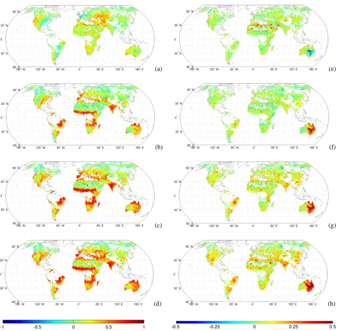
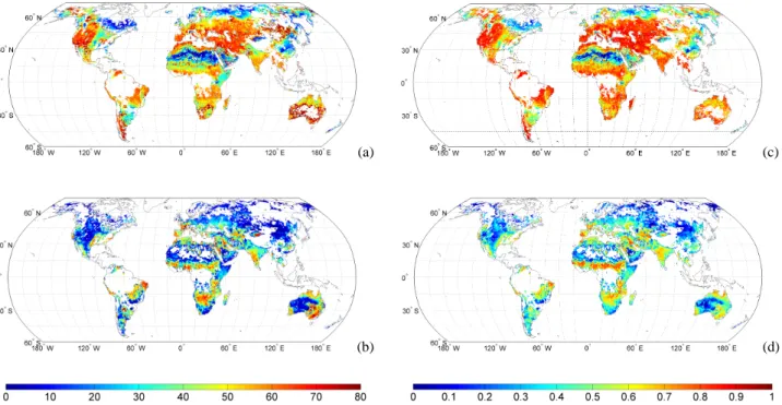
We analyzed the correlation between daily AMSR-E (LPRM) retrieved top-soil moisture and the different state variables representing different soil moisture quantities cal-culated in ORCHIDEE, on a daily time step. In Fig. 1a–d, the significant (p < 0.05) correlation coefficients are shown between AMSR-E (LPRM) and the ORCHIDEE variables SHALLOW SM, DEEP SM, TOT SM and ROOT SM. In the northern latitudes, AMSR-E (LPRM) is frequently not receiving a good signal because there is often snow on the ground, which leads to few reliable data points for the com-parison. Therefore, we applied a simple Land Surface Tem-perature filter to mask all cells with T < 273◦K (Holmes et al., 2009), and masked all cells with less than 100 (daily) data points per year. In areas with dense vegetation (optical depth > 0.8), AMSR-E (LPRM) is not reliable (Parinussa et al., 2011a) and therefore masked out completely.
It is clear that both modeled variables TOT SM and ROOT SM show the best correlation values with AMSR-E (LPRM) (Fig. 1c and d). SHALLOW SM and DEEP SM show somewhat opposite behavior. For dry areas the DEEP SM is very small and in fact interacts little with the surface since there is never the possibility of a merge between SHALLOW SM and DEEP SM. Therefore, in this case the model behaves like a single bucket model represented by the SHALLOW SM. This explains why we have a relatively good correlation between SHALLOW SM and AMSR-E (LPRM) and a poor correlation between DEEP SM and AMSR-E (LPRM) in dry regions. For others regions, the behavior of SHALLOW SM is more complex and can ap-pear or disapap-pear when merging with DEEP SM in a rela-tively random way which explains the poor correlation be-tween SHALLOW SM and AMSR-E (LPRM) and the good correlation between DEEP SM and AMSR-E (LPRM), be-cause SHALLOW SM drains into DEEP SM. Even though SHALLOW SM represents a shallow soil layer in the model, the correlation coefficient cannot be calculated at very dry times of the year, because this upper layer does not ex-ist and SHALLOW SM takes values equal to zero. There-fore, we do not use SHALLOW SM further in the analy-sis; rather, we continue with the ORCHIDEE output that showed the best correlation values, ROOT SM. In large ar-eas of Europe, East Europe, North America, South America and mid to south Africa, the correlation coefficient between
AMSR-E (LPRM) and ROOT SM is close to one, mean-ing that the temporal variability of the two products is very closely related. In the northern latitudes, the correlation co-efficient takes values between 0 and −1, which is caused by the fact that frozen soil in ORCHIDEE contains little water, while the water content is retrieved close to satura-tion in AMSR-E (LPRM). This is caused by the simple ap-plied mask, which has an uncertainty of ±4 K (Holmes et al., 2009), allowing soils to remain frozen when the surface tem-perature > 273◦K. In very dry areas (i.e. deserts), we find almost no correlation, since ORCHIDEE simulates no dif-ference in soil moisture, while AMSR-E (LPRM) has a high signal to noise ratio in these regions (De Jeu et al., 2008). The regions where ORCHIDEE and AMSR-E (LPRM) are closely related (r close to 1), correspond to a comparison of the European Remote Sensing Satellites (ERS) soil mois-ture products with soil moismois-ture output by the global dy-namic vegetation model LPJ (Wagner et al., 2003), as well as the comparison of AMSR-E (LPRM) with the global NOAH shallow soil moisture output (Liu et al., 2011b).
The anomaly analysis (Fig. 1e–h) shows much smaller correlation coefficients (range between −0.5–0.5) than the correlation between AMSR-E (LPRM) and the different state variables of ORCHIDEE, even though the general geo-graphic pattern is similar. This indicates that the inter-annual variability between AMSR-E (LPRM) and ORCHIDEE agree less, and part of the signal of the correlation coeffi-cient shown in Fig. 1a–d is caused by seasonality. Australia has a high anomaly correlation coefficient when comparing AMSR-E (LPRM) and ROOT SM. AMSR-E (LPRM) has been shown to have a good signal in this area (Draper et al., 2009; Mladenova et al., 2011), and ORCHIDEE input as well as soil description is probably very suitable for this region, causing an r of nearly 0.5. Although Southern Brazil has been shown to be a difficult area for AMSR-E (LPRM) (Dorigo et al., 2010), the inter-annual variability between AMSR-E (LPRM) and ROOT SM agree reasonably well.
Correlating the precipitation forcing (CRU-NCEP; with CRU at 0.5◦combined with NCEP at 1◦spatial resolution) to the AMSR-E (LPRM) soil moisture results in r-values be-tween −1 and 1 (Fig. 2). Correlation values are lower than AMSR-E (LPRM) compared with ORCHIDEE ROOT SM, which is caused both by the uncertainty of the precipitation field, and by the influence of land evaporation. Precipitation forcing fields are highly uncertain, and land surface models are most sensitive to this forcing to calculate soil moisture (Guo and Dirmeyer, 2006). New methods are being devel-oped to improve precipitation forcing along with soil mois-ture fields, e.g. using satellite-based rainfall accumulation estimates to improve surface soil moisture retrievals (Schu-mann et al., 2009), and sometimes including the use of hy-drological models (Crow et al., 2009; Parajka et al., 2009). Evaporation is highly important for the seasonal soil mois-ture cycle, as soil moismois-ture is not only driven by precipitation but also by soil water uptake (Miralles et al., 2011).
(a) (e)
(b) (f)
(c) (g)
(d) (h)
Fig. 1. (a)–(d): Global correlation coefficient maps of AMSR-E (LPRM) versus the ORCHIDEE soil moisture parameters SHALLOW SM, DEEP SM, TOT SM and ROOT SM for the time period 2002–2010. (e)–(h): Global correlation coefficient maps of the anomalies of AMSR-E (LPRM) versus the ORCHIDEE soil moisture parameters SHALLOW SM, DEEP SM, TOT SM and ROOT SM for the time period 2002–2010.
3.2.2 Evaluation with in situ data
The Pearson’s correlation coefficients between the soil mois-ture observations at the FLUXNET locations and AMSR-E (LPRM) and ROOT SM are shown in Table 2. AMRS-E (LPRM) and ROOT SM values are compared with available FLUXNET data between June 2002 and December 2007. The variability in correlation between in situ and mod-eled/satellite soil moisture is large, ranging from r = 0.13 in a cropland in Klingenberg, Germany, to r = 0.92 in a Pine for-est in CA, USA. We calculated the r of AMSR-E (LPRM)
with in situ data with and without a 5-day moving average on AMSR-E (LPRM), to see the difference when account-ing for the noise on AMSR-E (LPRM) and found that a 5-day moving average did not make a significant difference for these sites. No significant relation can be found between the value of the correlation coefficient and vegetation cover, and it seems that the order of the value of the correlation coeffi-cient is mainly determined by the existence of local processes such as land cover heterogeneity and subgrid precipitation events affecting each site. The correlation coefficients for
Table 2. Pearson’s correlation coefficient (r), and characteristic lag-times (ch. lag) in days of the FLUXNET in situ measurements, AMRS-E (LPRM) and ORCHIDEE (ROOT SM).
No Site Name In Situ AMSR-E (LPRM) ORCHIDEE (ROOT SM) N Period ch. lag r r(mov. av.)∗ r(ano.)∗ ch. lag r r(ano.)∗ ch. lag days
1 Lethbridge, Canada 33 0.33 0.44 0.48 5 0.51 0.13 59 804 Jul 2002–Jan 2006 2 Majadas del T, Spain 48 0.87 0.88 0.49 49 0.73 0.15 66 408 Jan 2005–Jan 2007 3 Vall dl Alinya, Spain 14 0.44 0.51 0.28 20 0.51 0.19 40 445 Mar 2004–Jan 2007 4 Le Bray, France 47 0.60 0.72 0.07 51 0.76 0.12 75 487 Jan 2005–Jan 2007 5 Dripsey, Ireland 51 0.44 0.65 0.09 2 0.79 0.63 45 437 Jan 2003–Jan 2006 6 Mitra IV Tojal, Port. 67 0.80 0.80 0.67 62 0.82 0.42 59 493 Jan 2005–Jan 2007 7 Pang/Lambourne, UK 60 0.54 0.76 0.19 19 0.89 0.07 71 593 Jan 2005–Jan 2007 8 Lamont, OK, USA 85 0.47 0.48 0.49 62 0.31 0.22 23 574 Jan 2003–Nov 2006 9 Hainich, Germany 55 0.46 0.53 0.47 23 0.81 0.49 65 1011 Jul 2002–Jan 2007 10 Tonzi Range, CA, USA 62 0.60 0.67 0.34 32 0.92 0.64 64 773 Jul 2002–Jan 2007 11 Mehrstedt, Germany 51 0.55 0.65 0.14 34 0.62 0.00 54 704 Sep 2003–Jan 2007 12 Hartheim, Germany 51 0.48 0.53 0.13 42 0.78 0.29 42 492 Jan 2005–Jan 2007 13 Klingenberg, Germany 10 0.43 0.43 0.45 9 0.13 0.15 66 393 Jan 2005–Jan 2007 14 Duke Forest, NC, USA 53 0.65 0.65 0.34 53 0.52 0.43 17 601 Jul 2003–Jan 2006 15 Metolius Pine, OR, USA 63 0.59 0.67 0.21 44 0.93 0.41 67 493 Jul 2004–Dec 2005
∗mov. av. = 5 day moving average, ano. = anomalies
Fig. 2. Global Pearson’s correlation coefficient maps of AMSR-E versus the CRU-NCEP precipitation forcing of ORCHIDEE.
ORCHIDEE are generally higher than for AMSR-E (LPRM) (on average 0.67 and 0.55 respectively), which may indicate that the FLUXNET measurements, which are taken in the top 30 cm, are more comparable to the depth of the ORCHIDEE root zone soil moisture than to the 2–5 cm surface soil mois-ture of AMSR-E. However, Cosh et al. (2006) suggest that at least 16 soil moisture stations are needed to obtain a reliable spatially averaged soil moisture value at a 0.25◦scale. Here, just a single observation is analyzed in comparison with 0.5◦ averaged satellite observations and care should be taken in the interpretation of these results. A temporal autocorrela-tion signature is likely to be spatially more stable and thus a more a powerful tool for data analysis when a dense soil moisture network is not present.
The soil moisture autocorrelation was calculated as the lag-k autocorrelation coefficient (rk) for the in situ
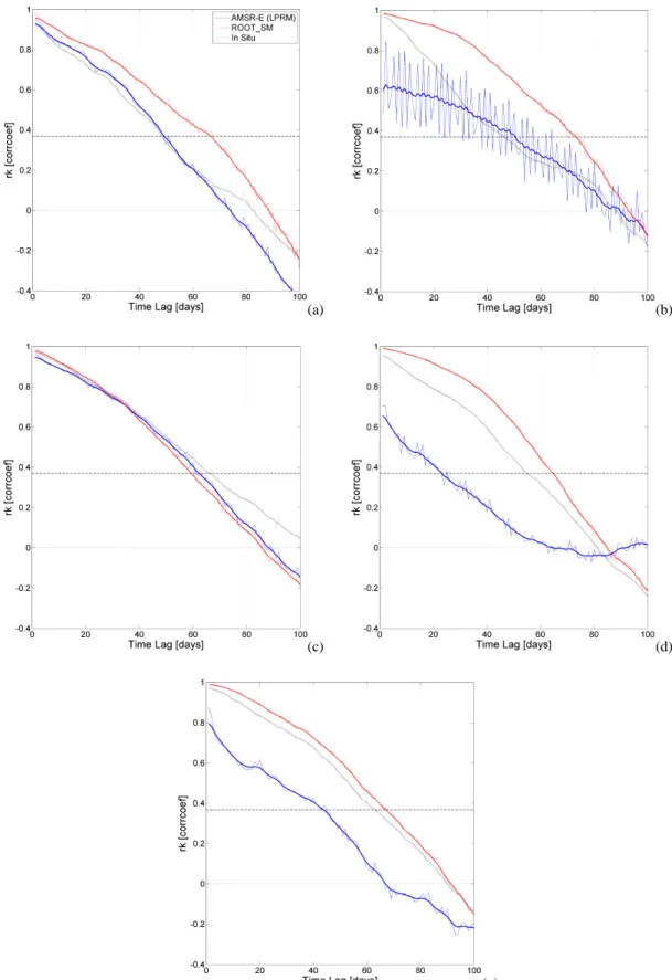
FLUXNET measurements, the satellite AMSR-E (LPRM) retrievals, and the ORCHIDEE ROOT SM simulated vari-able at each FLUXNET site (Tvari-ables 1 and 2). In Fig. 3, we
show the time series and in Fig. 4 the autocorrelation plots of these different variables for sites in Spain, France, Portugal, Germany and the USA. The time series shows the temporal dynamics of the different variables. In the autocorrelation plots (Fig. 4), on the y-axes rkis shown, which is a measure
of autocorrelation (Eq. 1). On the x-axes, the lag-time in days is shown for the corresponding autocorrelation values. The characteristic lag-time is the lag at which the autocorrelation function (rk) reduces to 1/e (0.37) (Delworth and Manabe,
1988; Maurer et al., 2001), which is represented by the black dashed horizontal line. For example, at the Portuguese site, AMSR-E (LPRM) (blue), ORCHIDEE (red) and the in-situ data (black) have a characteristic lag-time of around 60 days, which means that the “soil memory” is 60 days.
In Fig. 4, ORCHIDEE and FLUXNET show an excellent agreement in autocorrelation at the sites in Portugal, Ger-many and the USA, suggesting that the model captures the temporal dynamics of soil moisture on synoptic to seasonal scales well. On the other hand, AMSR-E (LPRM) has lower characteristic lag-times than FLUXNET data on the German and the USA sites, but agrees well on the Spanish, French and Portuguese sites. Annual rainfall and plant functional type do not seem to explain this behavior.
The time series for the in-situ FLUXNET measurements generally do not exceed a 2-year time period, which is too short for the anomaly autocorrelation calculation. However, we do have a 4.5 years-long time series for Hainich, Ger-many, for which we show the anomaly autocorrelation in Fig. 5. Even though the autocorrelation has a high similarity for in-situ and ORCHIDEE (Fig. 4), this signal is most likely dominated by the seasonal cycle as can be seen by the dissim-ilarity of in-situ and ORCHIDEE when addressing anomaly autocorrelation (Fig. 5). Figure 6 compares the in situ
(a) (b)
(c) (d)
(e)
Fig. 3. Time series of AMSR-E, ORCHIDEE ROOT SM and in situ FLUXNET soil moisture data of (a) Majadas del T, Spain (# 2), (b) Le Bray, France (# 4), (c) Mitra IV, Portugal (# 6), (d) Hainich, Germany (# 9) and (e) Metolius Pine, USA, (# 15).
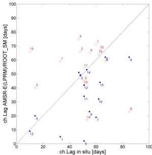
FLUXNET characteristic lag-time versus the characteristic lag-time of satellite AMSR-E (LPRM) soil moisture, and modeled ROOT SM variables, for the 15 sites. The cross-sites correlation coefficient of the characteristic lag-time be-tween in situ and AMSR-E (LPRM) is higher (r = 0.61), than the correlation coefficient of the characteristic lag-time be-tween in situ and ROOT SM (r = −0.16). This demonstrates a higher correspondence in the autocorrelation signature be-tween in situ FLUXNET and satellite observations, indicat-ing that both have a similar response to the hydrological pro-cesses. The autocorrelation signature of ROOT SM is sig-nificantly different, generally showing a lower temporal dy-namic in the model, mostly dictated by its sub-surface hy-drology. This can be expected from a mono-layer bucket, which is also indicative for the ORCHIDEE hydrology, since the top layer is often empty. Figure 6 shows that the model bias is rather constant for AMSR-E (LPRM), which always has a lower characteristic time than in-situ measurements. In contrast, ORCHIDEE generally has longer characteristic lag times than FLUXNET sites, except for two sites in the USA, Lamont, Oklahoma (740 mm yr−1 precip) and Duke forest,
North Carolina (1169 mm yr−1 precip). The longer charac-teristic lag-times by ORCHIDEE could be due to (1) unre-alistic (too smooth) rainfall forcing from CRU-NCEP model (i.e. underestimated precipitation variability because of unre-solved rainstorms; (2) structural rigidity in soil moisture dy-namics calculation of ORCHIDEE (i.e. not enough surface
runoff or lack of temporally variable root water uptake); in particular the unique deep soil layer imposes a single resi-dence time for water in the soil with respect to plant transpi-ration removal, whereas in reality, each soil layer has its own residence time; (3) misfit between modeled and observed soil moisture because ORCHIDEE only provides root-zone inte-grated values, which will show less variability than top-soil values, while AMSR-E (LPRM) and the measurements re-flect more shallow soil moisture dynamics, which are charac-terized by short term variability and thus short characteristic lag-times (Wu and Dickinson, 2004; De Lannoy et al., 2006). This is confirmed by Wagner et al. (1999) who found mean correlations between 0.35 to 0.53 and 0.33 to 0.49 when com-paring ERS scatterometer data with gravimetric soil moisture measurements in Ukraine in 0–20 cm and 0–100 cm layers respectively. The introduction of a multi-layer soil mois-ture model within ORCHIDEE with a better description of top-soil moisture dynamics might be a logical next step in model development. This could lead to a better assimilation of the entire soil moisture profile, which would result in a more direct one to one comparison with in situ and satellite observations.
3.2.3 Global autocorrelation maps
It is assumed that the autocorrelation function rkbecomes
in-significant when it takes values lower than 1/e, also shown in Figs. 4 and 5. In Fig. 7a and b, the characteristic lag-time
(a) (b)
(c) (d)
(e)
Fig. 4. Autocorrelation graphs of AMSR-E, ORCHIDEE ROOT SM and in situ FLUXNET soil moisture data of (a) Majadas del T, Spain (# 2), (b) Le Bray, France (# 4), (c) Mitra IV, Portugal (# 6), (d) Hainich, Germany (# 9) and (e) Metolius Pine, USA, (# 15). Black dashed horizontal line in autocorrelation graphs indicates where the rk value is equal to 1/e, indicating the characteristic lag-time at the x-axis.
Fig. 5. Anomaly autocorrelation for the Deciduous broadleaf forest site Hainich in Germany. Black dashed horizontal line in autocor-relation graph indicate where the rk value is equal to 1/e, indicating the characteristic lag-time at the x-axis, and where the rk value is equal to 0, indicating at which lag (x-axis) the autocorrelation has been lost.
is plotted on each grid point for 2002–2010. In general, the lag-time in ROOT SM is longer than in AMSR-E (LPRM), with differences of up to 50 days. Figure 7c and d show the autocorrelation value at a 20-day lag for ORCHIDEE ROOT SM (Fig. 7c) and AMSR-E (LPRM) (Fig. 7d). This shows a very similar trend as Fig. 7a and b, now showing that ORCHIDEE ROOT SM has high autocorrelation values at a 20-day lag, while AMSR-E (LPRM) autocorrelation has decreased to values below 0.4. Both analyses suggest a dis-crepancy due to the deeper soil depth in ROOT-SM, which produces a slower moisture removal after rain compared to AMSR-E (LPRM).
Overall, the slow decrease of soil moisture after rain in ORCHIDEE may suggest that this model will underestimate the response of vegetation to dry spells in the future, and hence may underestimate the positive feedback of climate change on the carbon cycle as well. In the recent coupled carbon-climate models intercomparison of Friedlingstein et al. (2006), ORCHIDEE indeed shows a smaller positive feed-back compared to other models. At face value, the too slow characteristic lag-time also reflects some inconsistency be-tween what is modeled (total soil moisture content) and what is observed (top-soil moisture). In that respect, it would help to incorporate a multi-layer soil hydrology in ORCHIDEE, as defined for instance by de Rosnay and Polcher (1998) and Orgeval et al. (2008).
Fig. 6. Characteristic lag-time of FLUXNET in situ soil moisture against characteristic lag-time of AMSR-E (blue) and ROOT SM (red). The numbers correspond to the site-numbers in Table 1.
4 Conclusions and summary
It has been shown that the daily soil moisture product of AMSR-E (LPRM) and simulations of ORCHIDEE forced by CRU-NCEP correlate well in time, within known errors of both, with correlation coefficients r greater than 0.6 for 30 % of the land area. However, correlation is known to be sensi-tive to outliers and general trends. When we study the tempo-ral characteristics of the two soil moisture products, they are quite different. Remotely sensed soil moisture has a much faster reaction time and much shorter characteristic lag-time than the soil moisture in ORCHIDEE. The characteristic lag-time of remotely sensed soil moisture corresponds well to the in-situ surface FLUXNET soil moisture. These results can be explained by the assumption that AMSR-E (LPRM) resents the upper 5 cm of soil at most, while ROOT SM rep-resents the root zone profile, generally the first meter of soil. In conclusion, we find that the remotely sensed soil moisture data compare well to the gridded soil moisture data modeled by the global dynamic vegetation model ORCHIDEE when looking at correlation, while they do not agree when also considering the temporal characteristics of the signal. The temporal response of ORCHIDEE to hydrological processes is different from the in situ and satellite observations.
This study demonstrates the potential to improve global land surface models with satellite soil moisture observations, because these observations appear to capture the existing temporal dynamics in soil moisture well. In the near future, satellite soil moisture observations might be used in a data as-similation routine to improve the soil moisture dynamics of the land surface model, similar to the assimilation of MODIS leaf area index (Demarty et al., 2007). This study shows that
(a) (c)
(b) (d)
Fig. 7. Global characteristic lag-time (days) for ORCHIDEE ROOT SM (a) and AMSR-E (LPRM) (b), as well as the autocorrelation value at a 20-day lag for ORCHIDEE ROOT SM (c) and AMSR-E (LPRM) (d).
this will most likely result in a better description of the bio-geochemical processes. Structural model developments to explicitly better account for soil moisture dynamics in the up-per soil layers (in particular a multilayered sub-surface soil-hydrology; de Rosnay and Polcher, 1998), would need to be executed to be able to assimilate the soil moisture data. This could result in a significant improvement of the terrestrial hy-drological cycle of the model. Global satellite soil moisture observations could be used as well to evaluate models for the characteristic drying times of soils after rainfall, a critical variable that will determine the future availability of moisture in soils in a warmer world, and hence the feedbacks between climate and the carbon cycle in coupled models.
Acknowledgements. The research leading to these results has
received funding from the European Community’s Seventh Framework Programme (FP7/2007-2013) under grant agreement no. 226701 (CARBO-Extreme). We also thank the PIs of the Fluxnet sites who allowed us to use their data for the validation of the model and satellite observations. The Metolius fluxnet site was funded by the US Department of Energy’s Office of Science (BER; grant DE-FG02-06ER64318).
Edited by: J. Liu
References
Albertson, J. D. and Kiely, G.: On the structure of soil moisture time series in the context of land surface models, J. Hydrol., 243, 101–119, 2001.
Angert, A., Biraud, S., Bonfils, C., Henning, C. C., Buermann, W., Pinzon, J., Tucker, C. J., and Fung, I.: Drier summers cancel out the CO2uptake enhancement induced by warmer springs, P.
Natl. Acad. Sci. USA, 102, 10823–10827, 2005.
Ashcroft, P. and Wentz, F.: AMSR-E/Aqua L2A Global Swath Spatially-Resampled Brightness Temperatures (Tb) V001, September to October 2003, National Snow and Ice Data Center, Digital media (Updated daily), Boulder, CO, USA, 2003. Baldocchi, D., Falge, E., Gu, L., Olson, R., Hollinger, D., Running,
S., Anthoni, P., Bernhofer, C., Davis, K., Evans, R., Fuentes, J., Goldstein, A., Katul, G., Law, B., Lee, X., Malhi, Y., Meyers, T., Munger, W., Oechel, W., Paw, K. T. U., Pilegaard, K., Schmid, H. P., Valentini, R., Verma, S., Vesala, T., Wilson, K., and Wofsy, S.: FLUXNET: A new tool to study the temporal and spatial variability of ecosystem-scale carbon dioxide, water vapor, and energy flux densities, B. Am. Meteorol. Soc., 82, 2415–2434, 2001.
Berbigier, P., Bonnefond, J. M., and Mellmann, P.: CO2and water vapour fluxes for 2 years above Euroflux forest site, Agr. Forest Meteorol., 108, 183–197, 2001.
Botta, A., Viovy, N., Ciais, P., Friedlingstein, P., and Monfray, P.: A global prognostic scheme of leaf onset using satellite data, Global Change Biol., 6, 709–725, 2000.
Casal, P., Gimeno, C., Carrara, A., L’opez-Sangil, L., and Sanz, M. J.: Soil CO2efflux and extractable organic carbon fractions under simulated precipitation events in a Mediterranean Dehesa, Soil Biol. Biochem., 41, 1915–1922, 2009.
Ciais, P., Reichstein, M., Viovy, N., Granier, A., Og´ee, J., Al-lard, V., Aubinet, M., Buchmann, N., Bernhofer, C., Carrara, A., Chevallier, F., De Noblet, N., Friend, A. D., Friedlingstein, P., Gr¨unwald, T., Heinesch, B., Keronen, P., Knohl, A., Krinner, G., Loustau, D., Manca, G., Matteucci, G., Miglietta, F., Ourcival, J. M., Papale, D., Pilegaard, K., Rambal, S., Seufert, G., Sous-sana, J. F., Sanz, M. J., Schulze, E. D., Vesala, T., and Valentini, R.: Europe-wide reduction in primary productivity caused by the heat and drought in 2003, Nature 437, 529–533, 2005.
Cosh, M. H , Jackson, T. J., Starks, P., and Heathman, G.: Tempo-ral stability of surface soil moisture in the Little Washita River watershed and its applications in satellite soil moisture product validation, J. Hydrol., 323, 168–177, 2006.
Crow, W. T., Huffman, G. F., Bindlish, R., and Jackson, T. J.: Improving satellite rainfall accumulation estimates using space-borne soil moisture retrievals, J. Hydrometeorol., 10, 199–212, 2009.
D’Andrea, F., Provenzale, A., Vautard, R., and De Noblet, N.: Hot and cool summers: Multiple equilibria of the continental water cycle, Geophys. Res. Lett., 33, L24807, doi:10.1029/2006GL027972, 2006.
d’Orgeval, T., Polcher, J., and de Rosnay, P.: Sensitivity of the West African hydrological cycle in ORCHIDEE to infil-tration processes, Hydrol. Earth Syst. Sci., 12, 1387–1401, doi:10.5194/hess-12-1387-2008, 2008.
De Jeu, R. A. M., Wagner, W. W., Holmes, T. R. H., Dolman, A. J., van de Giesen, N. C., and Friesen, J.: Global Soil Moisture Patterns Observed by Space Borne Microwave Ra-diometers and Scatterometers, Surv. Geophys., 28, 399–420, doi:10.1007/s10712-008-9044-0, 2008.
De Jeu, R. A. M., Holmes, T. R. H., Panciera, R., and Walker, J. P.: Parameterization of the Land Parameter Retrieval Model for L-Band Observations Using the NAFE’05 Data Set, IEEE Geosci. Remote S., 6, 630–634, doi:10.1109/LGRS.2009.2019607, 2009.
De Lannoy, G. J. M., Verhoest, N. E. C., Houser, P. R., Gish, T. J., and Van Meirvenne, M.: Spatial and tempo-ral characteristics of soil moisture in an intensively moni-tored agricultural field (OPE3), J. Hydrol., 331, 719–730, doi:10.1016/j.jhydrol.2006.06.016, 2006.
de Rosnay, P. and Polcher, J.: Modelling root water uptake in a complex land surface scheme coupled to a GCM, Hydrol. Earth Syst. Sci., 2, 239–255, doi:10.5194/hess-2-239-1998, 1998. Delworth, T. L. and Manabe, S.: The influence of potential
evapo-ration on the variabilities of simulates soil wetness and climate, J. Climate, 1, 523–547, 1988.
Demarty, J., Chevallier, F., Friend, A. D., Viovy, N., Piao, S., and Ciais, P.: Assimilation of global MODIS leaf area index re-trievals within a terrestrial biosphere model, Geophys. Res. Lett., 34, L15402, doi:10.1029/2007GL030014, 2007.
Don, A., Rebmann, C., Kolle, O., Scherer-Lorenzen, M., and Schultze, E-D.: Impact of afforestation-associated management changes on the carbon balance of grassland, Global Change Biol. 15, 1990–2002, doi:10.1111/j.1365-2486.2009.01873.x, 2009. Dorigo, W. A., Scipal, K., Parinussa, R. M., Liu, Y. Y., Wagner,
W., de Jeu, R. A. M., and Naeimi, V.: Error characterisation of global active and passive microwave soil moisture datasets, Hydrol. Earth Syst. Sci., 14, 2605–2616, doi:10.5194/hess-14-2605-2010, 2010.
Draper, C. S., Walker, J. R., Steinle, P. J., De Jeu, R. A. M., and Holmes, T. R. H.: Evaluation of AMSR-E derived soil moisture over Australia, Remote Sens. Environ., 113, 703–710, doi:10.1016/j.rse.2008.11.011, 2009.
Ducoudr´e, N. I., Laval, K., and Perrier, A.: SECHIBA, a new set of parameterizations of the hydrologic exchanges at the land-atmosphere interface within the LMD atmospheric general cir-culation model, J. Climate, 6, 248–273, 1993.
Flanagan, L. B. and Johnson, B. G.: Interacting effects of temper-ature, soil moisture and plant biomass production on ecosystem respiration in a northern temperate grassland, Agr. Forest Mete-orol., 130, 237–253, 2005.
Friedlingstein, P., Cox, P., Betts, R., Bopp, L., Von Bloh, W., Brovkin, V., Cadule, P., Doney, S., Eby, M., Fung, I., Bala, G., John, J., Jones, C., Joos, F., Kato, T., Kawamiya, M., Knorr, W., Lindsay, K., Matthews, H. D., Raddatz, T., Rayner, P., Reick, C., Roeckner, E., Schnitzler, K.-G., Schnur, R., Strassmann, K., Weaver, A. J., Yoshikawa, C., and Zeng, N.: Climate-Carbon Cycle Feedback Analysis: Results from the C4MIP Model Inter-comparison, J. Climate, 19, 3337–3353, 2006.
Gilmanov, T. G., Soussana, J. F., Aires, L., Allard, V., Ammann, C., Balzarolo, M., Barcza, Z., Bernhofer, C., Campbell, C. L., Cernusca, A., Cescatti, A., Clifton-Brown, J., Dirks, B. O. M., Dore, S., Eugste, W., Fuhrer, J., Gimeno, C., Gruenwald, T., Haszpra, L., Hensen, A., Ibrom, A., Jacobs, A. F. G., Jones, M. B., Lanigan, G., Laurila, T., Lohila, A., Manca, G., Marcolla, B., Nagy, Z., Pilegaard, K., Pinter, K., Pio, C., Raschi, A., Ro-giers, N., Sanz, M. J., Stefani, P., Sutton, M., Tuba, Z., Valentini, R., Williams, M. L., and Wohlfahrt, G.: Partitioning European grassland net ecosystem CO2exchange into gross primary
pro-ductivity and ecosystem respiration using light response function analysis, Agr. Ecosyst. Environ., 121, 93–120, 2007.
Guo, Z. and Dirmeyer, P. A.: Evaluation of the Sec-ond Global Soil Wetness Project soil moisture simulations: 1. Intermodel comparison, J. Geophys. Res., 111, D22S02, doi:10.1029/2006JD007233, 2006.
Holmes, T. R. H, De Jeu, R. A. M., Owe, M., and Dolman, A. J.: Land Surface Temperatures from Ka-Band (37 GHz) Pas-sive Microwave Observations, J. Geophys. Res., 114, D04113, doi:10.1029/2008JD010257, 2009.
Jaeger, L. and Kessler, A.: Twenty years of heat and water balance climatology at the Hartheim pine forest, Germany, Agr. Forest Meteool., 84, 25–36, 1997.
Jaksic, V., Kiely, G., Albertson, J., Katul, G., and Oren, R.: Net ecosystem exchange of grassland in contrasting wet and dry years, Agr. Forest Meteorol., 139, 323–334, 2006.
Kanamitsu, M., Ebisuzaki, W., Woollen, J., Yang, S.-K., Hnilo, J. J., Fiorino, M., and Potter, G. L.: NCEP-DEO AMIP-II Reanalysis (R-2), M. Bul. Atmos. Metol. Soc., 1631–1643, 2002.
Knohl, A., Schulze, E.-D., Kolle, O., and Buchmann, N.: Large carbon uptake by an unmanaged 250-year-old deciduous forest in Central Germany, Agr. Forest Meteorol., 118, 151–167, 2003. Koster, R. D., Dirmeyer, P. A., Guo, Z., Bonan, G., Chan, E., Cox, P., Gordon, C. T., Kanae, S., Kowalczyk, E., Lawrence, D., Liu, P., Lu, C., Malyshev, S., McAvaney, B., Mitchell, K., Mocko, D., Oki, T., Oleson, K., Pitman, A., Sud, Y. C., Taylor, C. M., Verseghy, D., Vasik, R., Xue, Y., and Yamada, T.: Regions of strong coupling between soil moisture and precipitation, Science, 305, 1138–1140, 2004.
Krinner, G., Viovy, N., De Noblet-Ducoudr´e, N., Og´ee, J., Polcher, J., Friedlingstein, P., Ciais, P., Sitch, S., and Prentice, I. C.: A dynamic global vegetation model for studies of the cou-pled atmophere-biosphere system, Global Biogeochem. Cy., 19, GB1015, doi:10.1029/2003GB002199, 2005.
Loveland, T. R., Reed, B. C., Brown, J. F., Ohlen, D. O., Zhu, Z., Yang, L., and Merchant, J. W.: Development of a global land cover characteristics database and IGBP DISCover from 1 km AVHRR data, Int. J. Remote Sens., 716, 1303–1330, 2000. Li, L., Njoku, E. G., Im, E., Chang, P. S., and St. Germaine, K.:
A preliminary survey of radio-frequency interference over the U.S. in Aqua AMSR-E data, IEEE T. Geosci. Remote, 42, 380– 390, 2004.
Liu, Y., Van Dijk, A. I. J. M., De Jeu, R. A. M., and Holmes, T. R. H.: An Analysis on Spatiotemporal Variations of Soil and Vegetation Moisture from a 29 year Satellite Derived Dataset over Mainland Australia, Water Resour. Res., 45, W07405, doi:10.1029/2008WR007187, 2009.
Liu, Y. Y., De Jeu, R. A. M., McCabe, M. F., Evans, J. P., and Van Dijk, A. I. J. M.: Global long-term passive microwave satellite-based retrievals of vegetation optical depth, Geophys. Res. Lett., 38, L18402, doi:10.1029/2011GL048684, 2011a.
Liu, Y. Y., Parinussa, R. M., Dorigo, W. A., De Jeu, R. A. M., Wag-ner, W., van Dijk, A. I. J. M., McCabe1, M. F., and Evans J. P.: Developing an improved soil moisture dataset by blending passive and active microwave satellite-based retrievals, Hydrol. Earth Syst. Sci., 15, 425–436, 2011b,
http://www.hydrol-earth-syst-sci.net/15/425/2011/.
Ma, S., Baldocchi, D. D., Xu, L., and Hehn, T.: Inter-annual vari-ability in carbon dioxide exchange of an oak/grass savanna and open grassland in California, Agr. Forest Meteorol., 147, 157– 171, 2007.
Maurer, E. P., O’Donnell, G. M., Lettenmaier, D. P., and Roads, J. O.: Evaluation of NCEP/NCAR reanalysis water and en-ergy budgets using macroscale hydrologic model simulations, in: Land surface hydrology, meteorology, and climate: ob-servation and modeling, edited by: Lakshmi, V., Albert-son, J., and Schaake, J., AGU, Washington, D.C., 137–158, doi:10.1029/WS003p0137, 2001.
Meesters, A. G. C. A., De Jeu, R. A. M., and Owe, M.: Analytical Derivation of the Vegetation Optical Depth from the Microwave Polarization Difference Index, IEEE Geosci. Remote S., 2, 121– 123, 2005.
Miralles, D. G., De Jeu, R. A. M., Gash, J. H., Holmes, T. R. H., and Dolman, A. J.: Magnitude and variability of land evaporation and its components at the global scale, Hydrol. Earth Syst. Sci., 15, 967–981, doi:10.5194/hess-15-967-2011, 2011.
Mitchell, T. D. and Jones, P. D.: An improved method of construct-ing a database of monthly climate observations and associated high-resolution grids, Int. J. Climatol., 25, 693–712, 2005. Mladenova, I., Lakshmi, V., Jackson, T. J., Walker, J. P., Merlin, O.,
and De Jeu, R. A. M.: Validation of AMSR-E Soil Moisture Us-ing L-band Airborne Radiometer Data from NAFE’06, Remote Sens. Environ., 115, 2096–2103, 2011.
Mo, T., Choudhury, B. J., Schmugge, T. J., Wang, J. R., and Jack-son, T. J.: A Model for Microwave Emission from Vegetation-Covered Fields, J. Geophys. Res., 87, 229–237, 1982.
Njoku, E. G. and Entekhabi, D.: Passive microwave remote sensing of soil moisture, J. Hydrol., 184, 101–129,
doi:10.1016/0022-1694(95)02970-2, 1996.
Njoku, E. G., Jackson, T. J., Lakshmi, V., Chan, T. K., and Nghiem, S. V.: Soil moisture retrieval from AMSR-E, IEEE T. Geosci. Remote, 41, 215–229, 2003.
Owe, M., De Jeu, R., and Holmes, T.: Multi-Sensor Climatology of Satellite-Derived Global Land Surface Moisture, J. Geophys. Res., 113, F01002, doi:10.1029/2007JF000769, 2008.
Parajka, J., Naeimi, V., Bl¨oschl, G., and Komma, J.: Matching ERS scatterometer based soil moisture patterns with simulations of a conceptual dual layer hydrologic model over Austria, Hydrol. Earth Syst. Sci., 13, 259–271, doi:10.5194/hess-13-259-2009, 2009.
Parinussa, R., Meesters, A. G. C. A., Liu, Y. Y., Dorigo, W., Wagner, W., and De Jeu, R. A. M.: An analytical solution to estimate the error structure of a global soil moisture data set, IEEE Geosci. Remote S., 8, 779–783, 2011a.
Parinussa, R. M., Holmes, T. R. H., Yilmaz, M. T., and Crow, W. T.: The impact of land surface temperature on soil mois-ture anomaly detection from passive microwave observations, Hydrol. Earth Syst. Sci., 15, 3135–3151, doi:10.5194/hess-15-3135-2011, 2011b.
Piao, S., Friedlingstein, P., Ciais, P., de Noblet-Ducoudr´e, N., Labat, D., and Zaehle, S.: Changes in climate and land use have a larger direct impact than rising CO2 on global river runoff trends, P.
Natl. Acad. Sci. USA, 104, 15242–15247, 2007.
Rayner, P. J., Scholze, M., Knorr, W., Kaminski, T., Giering, R., and Widmann, H.: Two decades of terrestrial Carbon fluxes from a Carbon Cycle Data Assimilation System (CCDAS), Global Bio-geochem. Cy., 19, GB2026, doi:10.1029/2004GB002254, 2005. Reichstein, M., Papale, D., Valentini, R., Aubinet, M., Bernhofer, C., Knohl, A., Laurila, T., Lindroth, A., Moors, E., Pilegaard, K., and Seufert, G.: Determinants of terrestrial ecosystem car-bon balance inferred from European eddy covariance flux sites, Geophys. Res. Lett., 34, L01402, doi:10.1029/2006GL027880, 2007.
Rodell, M, Houser, P. R., Jambor, U., Gottschalck, J., Mitchell, K., Meng, C. J., Arsenault, K., Cosgrove, B., Radakovich, J., Bosilovich, M., Entin, J. K., Walker, J. P., Lohmann, D., and Toll, D.: The global land data assimilation system, B. Am. Meteorol. Soc., 85, 381–394, 2004.
R¨udiger, C., Calvet, J. C., Gruhier, C., Holmes, T. R. H., De Jeu, R. A M., and Wagner W. W.: An Intercomparison of ERS-Scat, AMSR-E Soil Moisture Observations with Model Simulations over France, J. Hydrometeorol., 10, 431–448, doi:0.1175/2008JHM997.1, 2009.
Schmugge, T. J.: Remote sensing of soil moisture: Recent ad-vances, IEEE T. Geosci. Remote, 21, 336–344, 1983.
Schumann, G., Lunt, D. J., Valdes, P. J., de Jeu, R. A. M., Scipal, K., and Bates, P. D.: Assessment of soil moisture fields from imperfect climate models with uncertain satellite observations, Hydrol. Earth Syst. Sci., 13, 1545–1553, doi:10.5194/hess-13-1545-2009, 2009.
Seneviratne, S. I., Koster, R. D., Guo, Z., Dirmeyer, P. A., Kowal-czyk, E., Lawrence, D., Liu, P., Mocko, D., Lu, C., Oleson, K. W., and Verseghy, D.: Soil Moisture Memory in AGCM Simu-lations: Analysis of Global Land-Atmosphere Coupling Experi-ment (GLACE) Data, J. Hydrometeorol., 7, 1090–1112, 2006a. Seneviratne, S. I., L¨uthi, D., Litschi, M., and Sch¨ar, C.:
205–209, 2006b.
Sitch, S., Smith, B., Prentice, I. C., Arneth, A., Bondeau, A., Cramer, W., Kaplan, J. O., Levis, S., Lucht, W., Sykes, M. T., Thonicke, K., and Venevsky, S.: Evaluation of ecosystem dy-namics, plant geography and terrestrial carbon cycling in the LPJ dynamic global vegetation model, Global Change Biol., 9, 161– 185, 2003.
Solomon, S., Qin, D., Manning, M., Chen, Z., Marquis, M., Averyt, K. B., Tignor, M., and Miller, H. L.: Contribution of Working Group I to the Fourth Assessment Report of the Intergovernmen-tal Panel on Climate Change, Cambridge University Press, Cam-bridge, UK and New York, NY, USA, 2007.
Thomas, C. K., Law, B. E., Irvine, J., Martin, J. G., Pettijohn, J. C., and Davis, K. J.: Seasonal hydrology explains interannual and seasonal variation in carbon and water exchange in a semi-arid mature ponderosa pine forest in Central Oregon, J. Geophys. Res., 114, G04006, doi:10.1029/2009JG001010, 2009.
van der Schrier, G., Briffa, K. R., Osborn, T. J., and Cook, E. R.: Summer moisture availability across North America, J. Geophys. Res., 111, D11102, doi:10.1029/2005JD006745, 2006.
Wagner, W., Lemoine, G., and Rott, H.: A Method for Estimating Soil Moisture from ERS Scatterometer and Soil Data, Remote Sens. Environ., 70, 191–207, 1999.
Wagner, W., Scipal, K., Pathe, C., Gerten, D., Lucht, W., and Rudolf, B.: Evaluation of the agreement between the first global remotely sensed soil moisture data with model and precipitation data, J. Geophys. Res., 108, 4611, doi:10.1029/2003JD003663, 2003.
Wagner, W., Naeimi, V., Scipal, K., de Jeu, R., and Martinez-Fernandez, J.: Soil Moisture from Operational Meteorological Satellites, Hydrogeol. J., 15, 121–131, doi:1007/s10040-006-0104-6, 2007.
Wang, J. R. and Schmugge, T. J.: An empirical-model for the com-plex dielectric permittivity of soils as a function of water content, IEEE T. Geosci. Remote, 18, 288–295, 1980.
Wilks, D. S.: Statistical methods in the atmospheric sciences, Aca-demic Press, 51–54, 1995.
Wu, W. and Dickinson, R. E.: Time scales of layered soil mois-ture memory in the context of land-atmosphere interaction, J. Climate, 17, 2752–2764, 2004.