HAL Id: hal-02395959
https://hal.archives-ouvertes.fr/hal-02395959
Submitted on 8 Jan 2021
HAL is a multi-disciplinary open access
archive for the deposit and dissemination of
sci-entific research documents, whether they are
pub-lished or not. The documents may come from
teaching and research institutions in France or
abroad, or from public or private research centers.
L’archive ouverte pluridisciplinaire HAL, est
destinée au dépôt et à la diffusion de documents
scientifiques de niveau recherche, publiés ou non,
émanant des établissements d’enseignement et de
recherche français ou étrangers, des laboratoires
publics ou privés.
Distributed under a Creative Commons Attribution - NonCommercial| 4.0 International
720,000 years from Antarctic ice cores and climate
modeling
Kenji Kawamura, Ayako Abe-Ouchi, Hideaki Motoyama, Yutaka Ageta, Shuji
Aoki, Nobuhiko Azuma, Yoshiyuki Fujii, Koji Fujita, Shuji Fujita, Kotaro
Fukui, et al.
To cite this version:
Kenji Kawamura, Ayako Abe-Ouchi, Hideaki Motoyama, Yutaka Ageta, Shuji Aoki, et al.. State
dependence of climatic instability over the past 720,000 years from Antarctic ice cores and climate
modeling. Science Advances , American Association for the Advancement of Science (AAAS), 2017,
3 (2), pp.e1600446. �10.1126/sciadv.1600446�. �hal-02395959�
P A L E O C L I M A T E 2017 © The Authors, some rights reserved; exclusive licensee American Association for the Advancement of Science. Distributed under a Creative Commons Attribution NonCommercial License 4.0 (CC BY-NC).
State dependence of climatic instability over
the past 720,000 years from Antarctic ice cores
and climate modeling
Dome Fuji Ice Core Project Members: Kenji Kawamura,1,2,3* Ayako Abe-Ouchi,4,5* Hideaki Motoyama,1,2* Yutaka Ageta,6Shuji Aoki,7Nobuhiko Azuma,8Yoshiyuki Fujii,1,2 Koji Fujita,6 Shuji Fujita,1,2Kotaro Fukui,1†Teruo Furukawa,1,2 Atsushi Furusaki,9
Kumiko Goto-Azuma,1,2Ralf Greve,10 Motohiro Hirabayashi,1Takeo Hondoh,10Akira Hori,11 Shinichiro Horikawa,10‡Kazuho Horiuchi,12Makoto Igarashi,1Yoshinori Iizuka,10Takao Kameda,11 Hiroshi Kanda,1,2Mika Kohno,1§Takayuki Kuramoto,1Yuki Matsushi,13¶Morihiro Miyahara,14 Takayuki Miyake,1Atsushi Miyamoto,10Yasuo Nagashima,15Yoshiki Nakayama,16Takakiyo Nakazawa,7 Fumio Nakazawa,1,2Fumihiko Nishio,17Ichio Obinata,18Rumi Ohgaito,5Akira Oka,4Jun’ichi Okuno,1,2 Junichi Okuyama,10||Ikumi Oyabu,1Frédéric Parrenin,19Frank Pattyn,20Fuyuki Saito,5
Takashi Saito,21Takeshi Saito,10Toshimitsu Sakurai,1** Kimikazu Sasa,15Hakime Seddik,10 Yasuyuki Shibata,22Kunio Shinbori,10Keisuke Suzuki,23Toshitaka Suzuki,24Akiyoshi Takahashi,14 Kunio Takahashi,5Shuhei Takahashi,11Morimasa Takata,8Yoichi Tanaka,25Ryu Uemura,1,26 Genta Watanabe,27Okitsugu Watanabe,28Tetsuhide Yamasaki,14Kotaro Yokoyama,29
Masakazu Yoshimori,30Takayasu Yoshimoto31
Climatic variabilities on millennial and longer time scales with a bipolar seesaw pattern have been documented in paleoclimatic records, but their frequencies, relationships with mean climatic state, and mechanisms remain unclear. Understanding the processes and sensitivities that underlie these changes will underpin better understanding of the climate system and projections of its future change. We investigate the long-term characteristics of climatic variability using a new ice-core record from Dome Fuji, East Antarctica, combined with an existing long record from the Dome C ice core. Antarctic warming events over the past 720,000 years are most frequent when the Antarctic temperature is slightly below average on orbital time scales, equivalent to an intermediate climate during glacial periods, whereas interglacial and fully glaciated climates are unfavourable for a millennial-scale bipolar seesaw. Numerical experiments using a fully coupled atmosphere-ocean general circulation model with freshwater hosing in the northern North Atlantic showed that climate becomes most unstable in intermediate glacial conditions associated with large changes in sea ice and the Atlantic Meridional Overturning Circulation. Model sensitivity experiments suggest that the prerequisite for the most frequent climate instability with bipolar seesaw pattern during the late Pleistocene era is associated with reduced atmospheric CO2concentration via global cooling and sea ice formation in the North Atlantic, in addition to extended Northern Hemisphere ice sheets.
INTRODUCTION
Deep ice cores from Antarctica have provided records of climatic and environmental changes during the late Quaternary on 1000- to 100,000-year time scales (1–3). For the last glacial period, 25 millennial-scale Antarctic warming events [Antarctic Isotope Maximum (AIM)] have been identified as counterparts of abrupt climate changes in Greenland (Dansgaard-Oeschger events) (4, 5) and associated changes in hydrological cycles at lower latitudes (6). This is consistent with the bipolar seesaw hypothesis (7), in which changes of the Atlantic Meridio-nal Overturning Circulation (AMOC) modulate northward oceanic heat transport. Input of freshwater from ice sheets (icebergs or glacial melt) into the northern North Atlantic has been suggested as a cause of AMOC slowdown during glacial periods (8, 9). Documenting, understanding, and modeling the processes and sensitivities of these variabilities will aid in understanding the climate system and projections of its future change. However, the frequencies of millennial-scale climate variations in older glacial periods are inconsistent among studies and are therefore poorly constrained (3, 6, 10–13), thereby hampering the understanding of their relationships with mean climatic state and ultimate driving mecha-nisms (8–16). Problems in previous studies are partially attributable to the
lack of consistency through time due to decreasing time resolution with age for most paleoenvironmental archives.
Recent studies have used isotopic ratio (a temperature proxy) or mi-croparticle flux records from an 800–thousand year (ky) Antarctic ice core (Dome C) to suggest millennial-scale variability to be at its greatest in intermediate climatic states. However, these reported event identifi-cations are inconsistent with each other before 340 thousand years ago (ka) (13, 17). The time resolution of the water isotope record decreases with depth because of isotopic diffusion, which can greatly dampen small or fast signals in deep parts of the core (18). The microparticles do not undergo diffusion, yet their concentrations and deduced flux vary by an order of magnitude between glacial and interglacial periods, making it difficult to distinguish the climatic signal from analytical noise in warm periods. Investigation of millennial-scale variations based on the microparticle record has been limited to cold periods (17). There-fore, robustly documenting the frequency of climatic variability through multiple glacial cycles has required more than one long ice core. Here, we present a new ice-core record from Dome Fuji, Antarctica, which covers 720 ky (Fig. 1 and figs. S1 and S2). One advantage of this core is that the annual layers are two to three times thicker in its oldest glacial period than
on January 8, 2021
http://advances.sciencemag.org/
those in the Dome C core (fig. S3E), which enables higher sampling reso-lution and less diffusive smoothing of isotopic signals (see Materials and Methods) (18). By combining the isotope and microparticle records of the Dome Fuji and Dome C cores, it is possible to perform robust identi-fication and analysis of climatic variabilities and their relationship with background climatic state. We conduct numerical experiments with our atmosphere-ocean general circulation model (AOGCM) and analyze the results to interpret the ice-core data and investigate the dependence of cli-matic variabilities upon the background clicli-matic state.
RESULTS
There is a close resemblance between Dome Fuji d18O and Dome C dD records (both are interpreted as proxies for local air temperature above the boundary layer) on orbital and millennial time scales (Fig. 1).
For the present study, we aligned the chronology of the two cores using isotopic records and adopted the DFO-2006 time scale (2) where avail-able (for the past ~342 ky; 2500 m deep in the Dome Fuji core) and AICC2012 time scale (19) for the period before ~344 ky (see Materials and Methods and fig. S3). The transition from DFO-2006 to AICC2012 was made by linear interpolation of AICC2012 (see Materials and Methods). The age of the Dome Fuji core at 3028 m thus obtained is ~720 ky within the marine isotope stage (MIS) 17 interglacial period.
Microparticle flux in the Dome Fuji core was also analyzed and is shown in Figs. 1 and 2, together with the published Dome C record (17). The microparticle records are proxies for terrestrial dust input onto polar ice sheets (17). There are millennial-scale AIMs in MIS 16 (the oldest glacial period) (black arrows in Fig. 2) for which both the dust records show clear minima and are inversely correlated with the water isotope records. This suggests reduced aridity and/or weaker wind during Antarctic warming in South America, the dominant source of dust during glacial periods (20, 21). Thus, these AIMs are associated with hydrologic and atmospheric changes at lower latitudes, as seen in the last glacial period.
AIM amplitudes are generally small, so we made a composite iso-topic record from the Dome Fuji and Dome C cores to improve the signal-to-noise ratio (see Materials and Methods and Fig. 1E). In ad-dition, because the temporal resolution of the isotopic records de-creases with depth, we applied a low-pass filter (cutoff period, 3 ky) to the entire record. This was carried out to homogenize the resolution (Fig. 1F, red line) and to focus on detecting relatively large or distinct AIMs by setting constant thresholds to the first and second derivatives (see Materials and Methods and Fig. 1, H and I). The peak detection criteria were chosen to identify the nine AIMs in MIS 16. The cutoff period appeared reasonable considering that isotopic diffusion smooths out variations with periodicities shorter than a few thousand years in the deepest layers of the Dome C core (18). Identified peaks in the filtered curve were then compared with the Dome Fuji and Dome C isotopic and dust records, and only those with visible signals in all of the original data were accepted (see Materials and Methods for details). This led to the detection of 14 of 25 AIMs for the last glacial period and a total of 71 AIMs for the past 720 ky (Fig. 1G, red triangles). The reduced number in the last glacial period represents the magnitude of loss of resolution caused by ice thinning and isotopic diffusion, if these layers were to approach the bedrock.
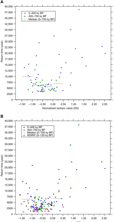
Proxy studies have suggested that climate instability and the asso-ciated bipolar seesaw become active in glacial periods (10, 13, 14). Here, we investigate the frequency of Antarctic climate variability and its re-lationship with mean climate state throughout the seven glacial cycles using our composite data. The relationship between the return time (pe-riod between two events) of AIM and Antarctic temperature proxy filtered on orbital time scales (Fig. 1F, gray line) reveals that the shortest median return time occurs when the temperature is slightly below av-erage in an intermediate glacial state (Fig. 3A) (13). Similar relationships were observed between AIM return time and sea level, although the results may be less robust because of relative chronological uncertainties (fig. S4). The distributions for two time windows (0 to 400 ky and 400 to 700 ky) are similar, suggesting that climatic instability did not notably change across the Mid-Brunhes Event ~430 ka, after which the ampli-tude of global ice volume and interglacial levels of Antarctic tempera-ture and atmospheric CO2content increased (3, 22). This suggests again that climate and ice sheets under intermediate glacial climate are relevant to the most frequent climate variability. These results are robust within a wide range of cutoff periods for the low-pass filter (figs. S5 and S6).
1
National Institute of Polar Research, Research Organizations of Information and Systems, 10-3 Midori-cho, Tachikawa, Tokyo 190-8518, Japan.2Department of Polar Science, Grad-uate University for Advanced Studies (SOKENDAI), 10-3 Midori-cho, Tachikawa, Tokyo 190-8518, Japan.3Institute of Biogeosciences, Japan Agency for Marine-Earth Science
and Technology, 2-15 Natsushima-cho, Yokosuka 237-0061, Japan.4Atmosphere and Ocean Research Institute, University of Tokyo, 5-1-5 Kashiwanoha, Kashiwa 277-8568, Japan.5Japan Agency for Marine-Earth Science and Technology, 3173-25 Showamachi,
Kanazawa, Yokohama, Kanagawa 236-0001, Japan.6Graduate School of Environmental Studies, Nagoya University, Furo-cho, Chikusa-ku, Nagoya 464-8601, Japan.7Graduate School of Science, Tohoku University, 6-3 Aramaki Aza-Aoba, Aoba-ku, Sendai 980-8578, Japan.8Department of Mechanical Engineering, Nagaoka University of
Technology, 1603-1 Kamitomioka, Nagaoka, Niigata 940-2188, Japan.9Asahikawa National College of Technology, 2-1-6, 2-jou, Syunkoudai, Asahikawa, Hokkaido 071-8142, Japan.10Institute of Low Temperature Science, Hokkaido University,
Kita-19, Nishi-8, Kita-ku, Sapporo 060-0819, Japan.11Department of Civil and Environmental Engineering, Kitami Institute of Technology, 165 Koen-cho, Kitami, Hokkaido 090-8507, Japan.12Graduate School of Science and Technology, Hirosaki
University, 3 Bunkyo-cho, Hirosaki, Aomori 036-8561, Japan.13Micro Analysis Lab-oratory, Tandem Accelerator, University of Tokyo, 2-11-16 Yayoi, Bunkyo-ku, Tokyo 113-0032, Japan.14Geo Tecs Co. Ltd., 1-5-14-705 Kanayama, Naka-ku, Nagoya
460-0022, Japan.15AMS Group, Tandem Accelerator Complex, University of Tsukuba,
1-1-1 Tennodai, Tsukuba, Ibaraki 305-8577, Japan.163D Geoscience Inc., Nogizaka Building, 9-6-41 Akasaka, Minato-ku, Tokyo 107-0052, Japan.17Center for Environmental
Remote Sensing, Chiba University, 1-33 Yayoi, Inage, Chiba 263-8522, Japan.18Obinata
Clinic, 3-2-1 Terazawa, Gosen, Niigata 959-1837, Japan.19Univ. Grenoble Alpes, CNRS, IRD, IGE, F-38000 Grenoble, France.20Laboratoire de Glaciologie, Faculté des Sciences,
CP160/03, Université Libre de Bruxelles, B-1050 Brussels, Belgium.21Disaster Prevention
Research Institute, Kyoto University, Gokasho, Uji, Kyoto 611-0011, Japan.22National Institute for Environmental Studies, 16-2 Onogawa, Tsukuba, Ibaraki 305-8506, Japan.
23Faculty of Science, Shinshu University, 3-1-1 Asahi, Matsumoto 390-8621, Japan. 24Faculty of Science, Yamagata University, 1-4-12 Kojirakawa-machi, Yamagata 990-8560,
Japan.25Geosystems Inc., Oshidate 4-11-20, Fuchu, Tokyo 183-0012, Japan.26Department of Chemistry, Biology, and Marine Science, University of the Ryukyus, 1 Senbaru, Nishihara, Okinawa 903-0213, Japan.27Chiken Consultants Co. Ltd., 11-27 Wakitahonmachi,
Kawagoe, Saitama 350-1123, Japan.28Graduate University for Advanced Studies, Shonan Village, Hayama, Kanagawa 240-0193, Japan.29Hokuriku Research Center, National
Agricultural Research Center, 1-2-1 Inada, Joetsu, Niigata 943-0193, Japan.30Faculty of
Environmental Earth Science, Global Institution for Collaborative Research and Education, and Arctic Research Center, Hokkaido University, Kita 10, Nishi 5, Kita-ku, Sapporo 060-0810, Japan.31IOK/Kyushu Olympia Kogyo Co. Ltd., Kunitomi-cho, Higashi-morokata-gun, Miyazaki
880-1106, Japan.
*Corresponding author. Email: kawamura@nipr.ac.jp (K.K.); motoyama@nipr.ac.jp (H.M.); abeouchi@aori.u-tokyo.ac.jp (A.A.-O.)
†Present address: Tateyama Caldera Sabo Museum, 68 Bunazaka-Ashikuraji, Tateyama-machi, Toyama 930-1305, Japan.
‡Present address: Earthquake and Volcano Research Center, Graduate School of Environmental Studies, Nagoya University, Furo-cho, Chikusa-ku, Nagoya 464-8601, Japan.
§Present address: Department of Geochemistry, Geoscience Center, University of Göttingen, Goldschmidtstr. 1, 37077 Göttingen, Germany.
¶Present address: Disaster Prevention Research Institute, Kyoto University, Gokasho, Uji, Kyoto 611-0011, Japan.
||Present address: Advanced Applied Science Department, IHI Co., Yokohama, Japan. **Present address: Civil Engineering Research Institute for Cold Region, Public Work Research Institute, Hiragishi, Toyohira-ku, Sapporo 062-8602, Japan.
on January 8, 2021
http://advances.sciencemag.org/
There are small AIMs undetectable in the above procedures, yet recognizable in individual records (dotted arrows in Fig. 2). As a sup-plementary analysis, using high-resolution data, albeit with reduced robustness, we visually identified small AIMs and added them to those detected in the above. Here, the Dome C dust record has the greatest amount of information because of its large variability and high sampling resolution. The Dome Fuji isotopic record has high resolu-tion in the oldest glacial period, and both isotopic records contain sim-ilar details in other periods. We therefore primarily inspected the Dome C dust record for additional AIMs and validated these AIMs with the Dome Fuji or Dome C isotope record without low-pass filtering (see Materials and Methods and fig. S7). This added 42 AIMs to those detected with the 3-ky filter (Fig. 1G, purple triangles). Median AIM return times decreased, as expected, and the conclusion that AIM is most frequent in intermediate glacial state still held (Fig. 3B). Compared with the aforementioned results, AIMs with a short
return time are clustered in the colder part of the intermediate glacial state (range of normalized isotopic value, −1.0 to −0.5), which is consistent with the distribution from the 25 Dansgaard-Oeschger events during the last glacial period (Fig. 3B).
We also found AIMs with long return time (>10,000 years) and great magnitude during deglaciations, when northern continental ice sheets disintegrate from their maximum extent, and during early parts of glacial periods when continental ice sheets are small (Fig. 1). From an accurate chronology, we previously showed (2) that the timings of large and infrequent AIMs in early glacial periods for the past three glacial cycles are consistent with precession variation, producing highly variable Northern Hemisphere summer insolation. This may suggest a role for orbital forcing in the interhemispheric seesaw, at least when orbital eccentricity is large. Long durations and large amounts of fresh-water input into the North Atlantic may be possible with strong increases in the Northern Hemisphere summer insolation (5, 23). This maintains –6 –4 –2 0 2 4
Dome Fuji and Dome C
isotope composite
(normalized to zero mean and
unit standard deviation)
700,000 600,000 500,000 400,000 300,000 200,000 100,000 0 Age (year BP) 0.01 0.1 1 10 100 (mg/ m
Dome C dust flux
2 /year) 0.01 0.1 1 10 100 (mg/m 2 /year) –1 × 10⁻³ 0 1 1st deriv ative (ky –1 ) –1 × 10⁻⁶ 0 1 2nd derivative (ky –2 ) −60 −58 −56 −54 −52 Dome Fuji δ (‰, VSMOW) 18 O –440 –420 –400 –380 Dome C δ D DF1 DF2 Cutoff period: 18 ky Cutoff period: 3 ky A B C D E F G H I
Mean (for isotope data)
Dome Fuji dus
t flux
(‰, VSMOW)
Fig. 1. Millennial-scale variability in water isotopes and dust flux records during the past 720,000 years for comparison of Dome Fuji ice-core data with Dome C data. (A) d18O record from DF1 core (pink) (1, 2) and DF2 core (red; this study) (see Materials and Methods). (B) dD record from Dome C core (19) relative to VSMOW (Vienna standard mean ocean water). (C) Dome Fuji dust flux. DF1 for younger part (53) and DF2 for older part (this study). (D) Dome C dust flux (17). (E) Composite isotope record. (F) Low-pass filtered isotope records [cutoff periods, 3 ky (red line) and 18 ky (gray line)] shifted downward by 4 units for visibility. (G) AIMs detected primarily using low-pass filtered isotopic composite (red triangles) and those with additionally detected events, primarily using the Dome C dust record (purple triangles) (see text). (H) First derivative of (F) (solid green line) and threshold for AIM detection (black dotted line). (I) Second derivative of (F) (solid green line) and threshold for AIM detection (black dotted line). For (A), (B), (E), and (F), gray dashed lines indicate means. For (C) and (D), thin dotted lines indicate raw data, and thick lines indicate the 1000-year running average. Note the inverted axis scale for (C) and (D). Age scale for all records is the combination of DFO-2006 for the last three glacial cycles and AICC2012 for the older period (see Materials and Methods). BP, before present.
on January 8, 2021
http://advances.sciencemag.org/
a negative ice-sheet mass balance (23), regardless of ice-sheet size and the existence of massive iceberg discharges (14, 24).
A question remains as to why the AMOC changes and bipolar see-saw are most frequent in the intermediate glacial state, in the absence of large orbital variations. To gain insight into the occurrence and dy-namics of the bipolar seesaw, we examined their dependence upon the background climatic state using our AOGCM called MIROC 4m (see Materials and Methods). The background climatic state in the model is established by forcings, such as atmospheric CO2content, ice-sheet size (extent and shape), and orbital configuration (25). We conducted 500-to 1000-year numerical experiments (so-called freshwater hosing experi-ments) under interglacial (preindustrial), midglacial, and full-glacial (16) conditions in which freshwater flux was added to the North Atlantic to examine climate stability, following classic methods (8, 9). Two cases of experiments, with small and large freshwater fluxes (0.05 and 0.10 sverdrup; 1 sverdrup = 106m3s−1) for 500 years, were executed to cover the range of estimated rate of sea-level rise associated with ice discharge events (see Materials and Methods and table S1) (26, 27).
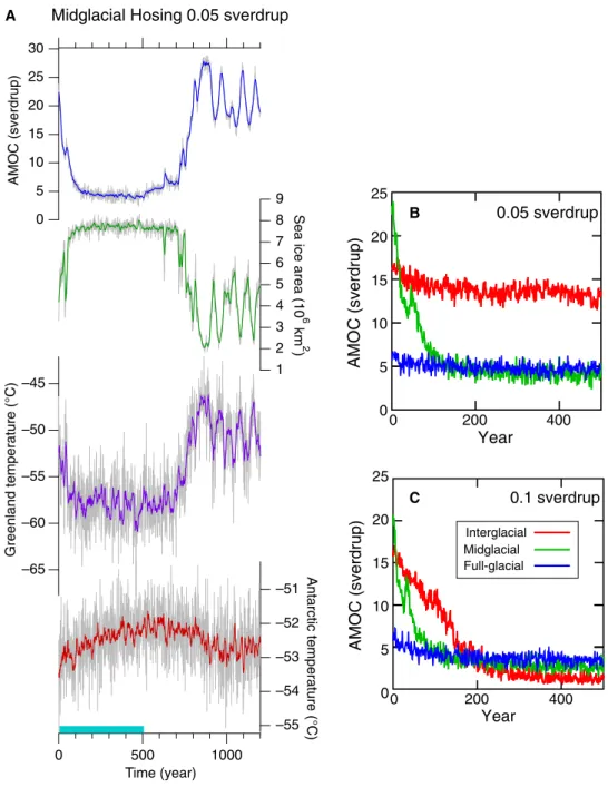
With both small and large amounts of freshwater input into the North Atlantic, the model simulates a clear bipolar seesaw pattern as-sociated with a weakening AMOC under the midglacial climatic con-dition, in contrast to results with the interglacial and full-glacial conditions (Figs. 4 and 5 and figs. S8 to S11). Our AOGCM results show that a strong response of climate to modest freshwater anomalies and the bipolar seesaw pattern occur most readily under intermediate glacial climate, consistent with our ice-core data.
The bipolar seesaw change is strongly related to the AMOC re-sponse to freshwater hosing, which is very different between the inter-glacial, midinter-glacial, and full-glacial simulations (fig. S11). The AMOC response to the small (0.05 sverdrup) freshwater anomaly in the inter-glacial and full-inter-glacial simulations is weak, whereas it is very strong in the midglacial simulation. This difference in AMOC behavior is closely related to the difference in the location of deep water formation and sea ice concentration in the North Atlantic (see Supplementary Notes). Under midglacial conditions, the model simulates decreases in surface salinity, surface density, and deep water formation; increases in sea ice cover in the North Atlantic; and a substantially weakened AMOC (figs. S11 and S12). Freshwater hosing into the cold surface water maintains extensive sea ice cover in the deep water formation region of the North Atlantic. Sea ice reduces the air-sea heat flux, thus halting deep convec-tion, weakening the AMOC, and cooling the North Atlantic surface air temperature (28–30). The AMOC weakening gradually warms the southern South Atlantic and the Southern Ocean (Fig. 5A and fig. S8), resulting in the bipolar seesaw.
Meanwhile, in the interglacial hosing simulation, the same amount of freshwater as above (0.05 sverdrup) is insufficient to form extensive sea ice in the North Atlantic to cover the convection region and ter-minate deep water formation (figs. S11B and S12B). Under the full-glacial condition, the freshwater does not have a great impact because convection in the North Atlantic is already weak before freshwater hosing (fig. S11E) and sea ice is very extensive compared with the in-terglacial or midglacial (fig. S12).
–60 –59 –58 –57 –56 –55 –54 Dome Fuji δ 18 O (‰, VSMOW) 700 690 680 670 660 650 640 630 620 Age (ky BP) –440 –430 –420 –410 –400 Dome C δD (‰, VSMOW) 0.01 0.1 1 10 Dust flux (mg/ m 2 /year ) Dome Fuji δ 18O Dome C δD Dome Fuji dust flux
Dome Fuji dust flux (3pt moving average) Dome C dust flux
Dome C dust flux (41pt moving average)
A
B
C
D
Fig. 2. Water isotope and dust flux records from Dome Fuji and Dome C in the oldest glacial period (MIS 16). (A) dD record from Dome C core (19). (B) d18O
record from DF2 core (this study). (C) Dome Fuji dust flux (this study). (D) EDC dust flux (17). Black arrows indicate nine millennial-scale AIMs identified in low-pass filtered isotopic curve (Fig. 1F). Dotted arrows indicate small AIMs visible in the high-resolution data. All records are on the AICC2012 age scale.
on January 8, 2021
http://advances.sciencemag.org/
Both the bipolar seesaw temperature pattern and the latitudinal evolution and rates of temperature change in our midglacial experi-ment (Figs. 4C and 5A) are consistent with ice-core data, paleoceano-graphic data, and conceptual studies (4, 7, 31, 32). In the Southern Ocean and Antarctica, in particular, the warming is gradual (a rate of ~1°C/500 year), with its onset lagging behind the abrupt Northern Hemisphere cooling by ~200 years (fig. S8) (31). At ~750 model years (~250 years after termination of the freshwater anomaly), the North-ern Hemisphere abruptly warms on a decadal time scale, whereas Antarctica continues warming for another 100 to 200 years before the temperature peaks and begins cooling (fig. S8).
Our model also simulated a clear response of the hydrologic cycle, namely, a southward shift of the low-latitude rain belt or Intertropical Convergence Zone (ITCZ) (9, 33) and an increase of precipitation over most of the Southern Hemisphere under the midglacial climate (Fig. 4D). The model results also showed a decrease in wind speed over the Southern Ocean (fig. S10) in response to the freshwater hosing. These are both believed to reduce dust flux to Antarctica un-der the glacial conditions with freshwater hosing, consistent with the observed anticorrelation between temperature and dust flux.
To understand the process of the clear bipolar climate change and AMOC response to a small freshwater anomaly under midglacial conditions, we ran additional sensitivity experiments, in which only (i) atmospheric greenhouse gases or (ii) continental ice sheets were set to the midglacial level with other conditions identical to those of the interglacial. In the first experiment, through greenhouse gas– induced global cooling, the AMOC was partially weakened not only because of sea ice expansion in the Northern Hemisphere (34) but also because of Antarctic cooling via its influence on the buoyancy of bottom waters (3, 35). With freshwater hosing of 0.05 sverdrup, the experiment shows substantial cooling and sea ice expansion in the Northern Hem-isphere, strong weakening of the AMOC, and a clear bipolar pattern similar to the midglacial simulation (Fig. 4, C and G, and fig. S11, C, D, G, H, and K). In contrast, in the second experiment, the AMOC did not weaken with the freshwater hosing, indicating strong AMOC stability as in the interglacial simulation. Because of the interglacial greenhouse gas forcing, the sea ice extent is small, and therefore, strong convection can occur in the North Atlantic (fig. S12, I and J). On the other hand, the large ice sheet strengthens the Icelandic Low and wind stress over the North Atlantic and promotes vigorous salt advection from low latitudes, resulting in strengthening of the AMOC (36). AMOC response to freshwater hosing was the smallest among all experiments (fig. S11). These sensitivity experiments suggest that a key background condition for frequent climate variability under intermediate glacial conditions is reduced CO2, which cools the high latitudes of both hemispheres.
DISCUSSION
Given the above, our ice-core data and model suggest that a great sen-sitivity of climate and the AMOC under the intermediate glacial conditions are necessary for strong climatic instability with the bipolar seesaw pattern. Key features of those conditions may be a stronger AMOC state (before freshwater forcing) than under the full-glacial conditions and a cooler global climate than under the interglacial conditions, as indicated by our model. This is consistent with a recent paleoceanographic finding of frequent AMOC oscillation between strong and weak modes during the last glacial period (37). For the full-glacial state, our model result indicates that the convections in
40,000 37,500 35,000 32,500 30,000 27,500 25,000 22,500 20,000 17,500 15,000 12,500 10,000 7500 5000 2500 0
Return time (year)
2.50 2.00 1.50 1.00 0.50 0.00 –0.50 –1.00 –1.50
Normalized isotopic value (SD) 0–400 ky BP 400–700 ky BP Median (0–700 ky BP) 40,000 37,500 35,000 32,500 30,000 27,500 25,000 22,500 20,000 17,500 15,000 12,500 10,000 7500 5000 2500 0
Return time (year)
2.50 2.00 1.50 1.00 0.50 0.00 –0.50 –1.00 –1.50
Normalized isotopic value (SD) 0–400 ky BP 400–700 ky BP Median (0–700 ky BP) NGRIP (0–120 ky BP) A B
Fig. 3. Frequency of AIM and its relationship with Antarctic temperature. Return time of AIM plotted against the composite Antarctic isotope record filtered on orbital time scales (Fig. 1F) for 0 to 400 ky (blue circles) and 400 to 700 ky (green diamonds). Median values of return time are plotted as horizontal bars. (A) From AIMs detected in 3-ky low-pass filtered isotopic composite with constant thresholds for the first and second derivatives, with validation by dust records. (B) From AIMs detected using Dome C dust record and validation by unsmoothed isotopic records through visual inspection. Return time for abrupt warming in Greenland (on DFO-2006 time scale) is also plotted (red squares). In each panel, the value of zero on horizontal axis indicates the mean of isotopic composite curve, corresponding to−57.13‰ for Dome Fuji d18O and−421.3‰ for Dome C dD records.
on January 8, 2021
http://advances.sciencemag.org/
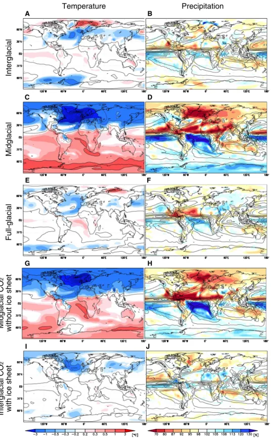
Temperature Precipitation Interglacial Midglacial Full-glacial Midglacial CO 2
without ice sheet
Interglacial CO
2
with ice sheet
A B C D E F G H I J ° ° ° ° ° ° ° ° ° ° ° ° ° ° ° ° ° ° ° ° ° ° ° ° ° ° ° ° ° ° ° ° ° ° ° ° ° ° ° ° ° ° ° ° ° ° ° ° ° ° ° ° ° ° ° ° ° ° ° ° ° ° ° ° ° ° ° ° ° ° ° ° ° ° ° ° ° ° ° °
Fig. 4. Results of MIROC freshwater hosing simulations (0.05 sverdrup) for temperature and precipitation. (A) Map of atmospheric temperature difference and (B) precipitation difference between hosing and control experiments for interglacial climate (mean for 400 to 500 model years after onset of hosing, which is the last 100 years of the“hosing” period). As in (A) and (B), but for (C and D) midglacial climate and (E and F) full-glacial climate. As in (A) and (B), but for sensitivity experiment of (G and H) midglacial climate“without” ice sheet and for (I and J) interglacial climate “with” ice sheet. In the left panels, solid line (dashed line) contours are drawn for every degree Celsius of temperature increase (decrease). The right panels show the same climatological pattern (preindustrial, contour lines) and anomaly in % (colors) caused by freshwater hosing (mean for 400 to 500 model years) for each climate state.
on January 8, 2021
http://advances.sciencemag.org/
the North Atlantic and AMOC are already weak in the background state (35, 37, 38), therefore limiting the impact of freshwater forcing. Therefore, infrequent AIMs may be attributed not only to mostly pos-itive ice-sheet mass balance (23), causing smaller numbers and amounts of freshwater releases than in the middle glacial state, but also to reduced sensitivity of the AMOC and climate. We note that these behaviors of sea ice and AMOC need to be validated with pa-leoclimatic data and other climate models (25).
Under initially strong AMOC mode, once the AMOC weakens be-cause of modest freshwater input, sea ice covers the main deep water
formation area in the North Atlantic, which, in turn, abruptly weakens the AMOC and intensifies cooling. Our model results are consistent with paleoclimatic data and theory, which propose that the climate change signal from the northern North Atlantic rapidly propagates through the ocean to midlatitudes of the South Atlantic (near the west coast of South Africa) by Kelvin and Rossby waves (7, 32, 33). The gradual warming in the Southern Ocean and Antarctica was demon-strated for the first time in an AOGCM with a reasonable amount of freshwater perturbation. This gradual warming could be caused by ed-dy mixing and deep oceanic mixing (instead of wave propagation) that
0 5 10 15 20 25 0 200 400 B AMOC (sverdrup) Year 0.05 sverdrup C Year 0.1 sverdrup 0 200 400 Interglacial Midglacial Full-glacial 0 5 10 15 20 25 AMOC (sverdrup)
A Midglacial Hosing 0.05 sverdrup
30 25 20 15 10 5 0 sverdrup)( C O M A Greenland temperature (°C) Antarctic temperature (°C) 1000 500 0 Time (year) 9 8 7 6 5 4 3 2 1 0 1( a er a e ci a e S 6 m k 2 ) –65 –60 –55 –50 –45 –55 –54 –53 –52 –51
Fig. 5. Time evolution results of the MIROC climate model simulation with freshwater hosing. (A) Top to bottom: Time series of maximum AMOC strength, North Atlantic sea ice extent (February sea ice of 90% concentration), and atmospheric temperature (2 m above the surface) at Greenland summit (average from December to February) and Dome Fuji (Antarctica, annual mean) under the midglacial climate after the onset of freshwater hosing of 0.05 sverdrup. The freshwater anomaly is applied for 500 years (shown as blue bar above the time axis) and then switched off, and the integration continues for an additional 700 model years (total simulation run of 1200 years is shown). (B) Maximum AMOC strength of the three experiments for the 500 years after the onset of 0.05-sverdrup hosing (red, interglacial; green, midglacial; blue full-glacial). (C) Maximum AMOC strength as in (B) for the case of 0.1-sverdrup hosing.
on January 8, 2021
http://advances.sciencemag.org/
transport heat across the Southern Ocean, where a meridional topo-graphic boundary is absent (33). The AMOC weakening may be pro-longed by ice discharge from the continental ice sheets through subsurface warming in the North Atlantic (39, 40), but freshwater should eventually cease because of North Atlantic cooling and/or de-pletion of ice from continental margins. After the end of the freshwater perturbation, the AMOC and thus climate in the Northern Hemisphere could abruptly recover to background states, with consequent onset of cooling in the Southern Ocean and Antarctica. Although the ultimate trigger is not known, our results are consistent with the hypotheses that the climatic oscillation may have been caused by weak forcing [so-called stochastic resonance (8, 41)] and/or by the coupling of northern ice sheets and AMOC (39, 42). We suggest that the required freshwater input for AMOC weakening is smallest under the intermediate glacial conditions because of cooling in both polar regions by reduced greenhouse gas forcing relative to the interglacial and early glacial conditions. From the persistent relationship in ice-core data between climate variability and Antarctic temperature, along with our consistent model results, we em-phasize the importance of greenhouse gas forcing as a determining factor in the stability of AMOC and global climate, in addition to the existence of Northern Hemisphere ice sheets.
The long return time and pronounced interhemispheric seesaw may also have been produced by high-amplitude boreal summer in-solation, as observed in some early glacial and deglacial periods. High summer insolation might have produced substantial ice-sheet melt and induced great changes in the AMOC and climate, as seen in our model results with 0.1-sverdrup freshwater hosing under inter-glacial and midinter-glacial conditions. Our results also have implications with regard to the future climate (43). Recent studies using oceano-graphic observations and paleoceanooceano-graphic reconstructions have found substantial AMOC weakening over the last few decades, al-though the cause for this is not well understood (44–46). In this con-text, special attention should be paid to the required freshwater flux for AMOC weakening from its strong mode. Our results suggest that, if a large freshwater flux from the Greenland ice sheet occurs in the future, AMOC weakening could be amplified. Further studies are needed on the stability of AMOC—with particular focus on its rela-tionship with sea ice and the polar climate under the changing background climate from past to present—to enhance understanding of the climate system and its future changes.
MATERIALS AND METHODS
Dome Fuji ice core
Dome Fuji is one of the dome summits in East Antarctica (77°19′01″S, 39°42′12″E; altitude, 3810 m above sea level; fig. S1), located on the polar plateau facing the Atlantic and Indian Ocean sectors. The dome is surrounded by the Dronning Maud Mountains, a coastal escarp-ment along longitudes 20°W to 35°E. The present Dome Fuji is under a spatial gradient of surface mass balance decreasing southward (47). Two deep ice cores have been drilled there. Ice thickness at the site was estimated at 3028 ± 15 m (48). The present-day mean annual air temperature and snow accumulation rate are−54.4°C (49) and 27.3 ± 1.5 kg m−2year−1(50), respectively. The first ice core (DF1) was drilled to depth 2503 m by December 1996 (51), at which time the drill became stuck. The DF1 core has provided records of climatic and environmental changes over the past 340 ky (1, 2, 48, 52–54). The second core (DF2) was drilled 44 m from the first borehole, reaching 3035.22 m in January 2007 (55). Although the bedrock was not reached,
small rock fragments found in the ice from the deepest drill runs sug-gested that the bedrock was near the borehole bottom (55). We also found evidence of basal melting from a large amount of refrozen meltwater in the core barrel and chip chamber of the drill, confirming a suggestion from a three-dimensional ice-sheet flow model (56). Basal melting was later confirmed on the basis of radar sounding (57). Layer inclination in the Dome Fuji ice core
Inclination of visible layers within the DF2 core, such as tephra layers and cloudy bands, was measured with a protractor. The SE of the mea-surement was ~5°. Layers in the Dome Fuji ice core progressively in-clined at depths greater than ~2400 m, and the inclination reached ~50° near the bedrock. In addition, the inclination record shows stepwise changes at ~2600, ~2800, ~2900, and <~2950 m (fig. S2B). These changes were unexpected because the coring site was selected to be above the sub-glacial basin, and no highly irregular bedrock topography was ob-served in the vicinity (48). For example, the map showing the present state of the bed topography (fig. S14) suggests that the steepest slope within a few kilometers of the coring site is at most 10°. Two one-dimensional ice flow modeling studies (58, 59) and three-dimensional ice-sheet flow models (56, 60) covering the Dome Fuji coring site showed that alternative conditions of basal melting or freezing are sen-sitive to the choice of geothermal heat flux, which crucially affects the age of the ice near the bottom. More recently, anomalous increases of the electromagnetic reflectivity at the subglacial bed associated with the presence of subglacial water were detected (57). These features were used to delineate frozen and temperate beds in this area (red dotted lines in fig. S14). The beds of the inland part of the ice sheet tend to be temperate, with the exception of subglacial high mountains.
On the basis of these factors, several explanations are proposed for the large inclination and stepwise changes observed. The large inclina-tion can be attributed to spatially inhomogeneous occurrences of basal melting. The temperature of the ice core was at the pressure melting point. This was predicted in a previous modeling study (56), in which ice was estimated to freeze along the bed of mountainous areas near the coring site (61). In addition, the bedrock topography maps show that the drilling site is close to the boundaries between frozen and temperate beds in fig. S14. The stepwise changes of the layer inclina-tion require time-series changes under dynamical condiinclina-tions. Potential causes of those changes are hypothesized to be (i) cyclical changes in stress/strain configurations as a result of evolution of the Antarctic ice sheet during glacial/interglacial periods, (ii) cyclical changes in area and amount of basal melting as a result of periodic changes in bottom temperature over glacial/interglacial periods (56), and/or (iii) episodic subglacial drainage events initiated and sustained by small changes in surface slope (62). We assume that the subglacial water system and melting played an important role. Radar-sounding data indicated that the bed of the subglacial trench (blue; 10-km-wide area in fig. S14) is wet, implying the presence of subglacial lakes in the vicinity. An earlier airborne radar survey (63) reported a 20-km-long subglacial lake located 45 km west-southwest from Dome Fuji (77°30′S, 37°26′E; bed elevation, 645 m above sea level). By radar sounding, we confirmed that this lake system is connected to the subglacial trench in fig. S14. We speculate that the water system in the main basin beneath Dome Fuji causes spatially inhomogeneous and time-dependent basal melting. Measurement of d18O using sawdust samples
The DF2 d18O at depths below 2400 m was measured in sawdust samples (fine ice chips produced from longitudinal cutting of the
on January 8, 2021
http://advances.sciencemag.org/
ice core) that were continuously collected at Dome Fuji with 50-cm resolution. All DF2 d18O samples were collected and sealed in plastic bags and transported frozen to Japan. They were melted at the Nation-al Institute of Polar Research (NIPR) before anNation-alysis. d18O was measured with a mass spectrometer (Finnigan MAT DELTAplus) at NIPR, using the isotope equilibration technique (64) with analytical precision (1s) of 0.05‰. The DF2 sawdust d18O data agree well with the DF1 d18O data measured using ice (1, 48) across the overlapping depth interval (2400 to 2500 m). The quality of the d18O data is thus adequate for examination herein.
Measurement of microparticles
Microparticles (insoluble dust) were analyzed using a laser particle counter in 0.1-m-long DF2 ice samples, cut at the NIPR in 0.5-m depth intervals between 2400 and 3028 m (DF2 depths). For decontamination, the 3-mm surface of the samples was scraped off with a precleaned ceramic knife. The samples were then melted in contamination-free plastic bags. The first fraction of melt was discarded, and the rest was used for analysis. Number concentrations and size distribution of microparticles (0.52 to 3.11 mm diameter) were measured using a nine-channel laser particle counter (model 211, Met One Inc.) with an improved method based on our previous work (53). Raw data from a previous study (53) were used for the DF1 core but were recalibrated with a new calibration curve that was used for DF2 measurement. Moreover, the raw data were carefully examined, and outliers and data apparently affected by air bubbles were removed. Microparticle flux was derived using calculated mass concentrations and estimated snow accumulation rates. To calculate the mass concentrations, density was taken as 2500 kg m−3. Despite the relatively large analytical error in our microparticle analysis (~40% in individual samples), we could clearly identify millennial-scale variability in cold climate, which was much larger than the error (Figs. 1 and 2).
Integrity of the Dome Fuji ice core
The oxygen isotopic composition (d18O) of the ice, layer inclination angles, and borehole tilt angles of the Dome Fuji cores are plotted against depth in fig. S2. The values of d18O from the DF1 and DF2 cores agree across the overlapping depth interval (2403 to 2503 m), with depths from DF2 shifted downward by 3 m. This depth offset may be accounted for by the combination of layer inclination (~5°; fig. S2B) and tilt of the two boreholes (<1°). At greater depths, the layer inclination gradually increases with stepwise changes, reaching ~50° near the bottom of the core (borehole tilt remains <6°). We spec-ulate that the large inclination developed as a result of spatially in-homogeneous basal melting. One- and three-dimensional ice flow models (56, 58, 59, 61) suggest that the basal condition (melting or freezing) is very sensitive to geothermal heat flux. The stepwise incli-nation increases may have been caused by variations in physical conditions near the bed, for example, basal melting, stress/strain conditions, and/or changes in the distribution of subglacial meltwater over the course of glacial-interglacial cycles (see below for details). This raises the concern that the stratigraphy near the bottom of the core might be affected by irregular ice flow; however, we never ob-served discontinuity or folding of the layers, and the crystal orientation fabrics were continuous. Moreover, the DF2 d18O profile is very sim-ilar to that of Dome C (Fig. 1 and fig. S3). These observations indicate that layer thinning of the Dome Fuji core in the lower 200 m was greatly reduced as a result of basal melting, but this did not disturb the strati-graphy. As a result, the Dome Fuji core contains annual layers that are
up to three times thicker than those in the Dome C core in MIS 16 (the oldest glacial period covered by our core; Fig. 2).
Chronology and stacking
A common time scale for the Dome Fuji and Dome C cores was established to compare and stack their isotopic records. For this study, we adopted the DFO-2006 time scale (2) for the past ~342 ky and the AICC2012 time scale (19, 65) for the period older than ~344 ka. Features of the DFO-2006 and AICC2012 time scales and their rela-tionships for the last 220 ky are discussed by Fujitaet al. (66).
The DF1 d18O record used for the synchronization is a 100-year resampled data set from unsmoothed raw data (1), corrected for a few errors in the original data set (in digitizing depth or d18O values) (2). A preliminary time scale all along the Dome Fuji core was first calculated with a one-dimensional ice flow model (58) using six age control points from DFO-2006 (at 345, 791, 1262, 1699, 2103, and 2500 m, corresponding to 11.2, 41.2, 81.9, 126.4, 197.3, and 339.4 ky, respectively) and two points from AICC2012 (at 2750 and 3000 m, corresponding to 533.0 and 705.0 ky, respectively, through visual matching of the DF and EDC isotopic records). For this calculation, we corrected the Dome Fuji d18O for changes in mean oceanic isotopes [following the study of Parreninet al. (58)], but we did not correct the data for changes in water vapor source temperature because dD data are not yet available all along the core [note that the same approach was used for the Dome C core (19)]. The differences of modeled ages from the respective control ages are smaller than 1.5 ky, and the resulting parameters for the accumulation and ice flow models (58) are as follows: A0(near-surface accumulation rate), 2.753 cm of ice year−1; b (constant in exponential function for the accumulation model), 0.1188;p (parameter for the vertical profile of deformation), 7.54009; m (basal melting rate), 0.14401 mm/year; ands (sliding ratio), −1.97116 [see the study of Parreninet al. (58) for the explanation of the models and parameters]. The combined Dome Fuji time scale (DFO-2006 extended by the preliminary time scale for the deeper part; fig. S3A) was then matched with AICC2012 (fig. S3B) using Match software (67). For this software, manual matching points were placed at 13 ages (fig. S3), and adjustable parameters were set as follows: number of intervals, 800; end point pen-alty, 14; speed penpen-alty, 0.7; speed change penpen-alty, 0.5; tie point penpen-alty, 0.1; and gap size penalty, 0.1. These parameters were determined using automatic adjustment of the software and then adjusted manually by visual examination of the overall result. Most glacial inceptions (black segments in the Dome Fuji isotopic curve of fig. S3A) were excluded from the matching, owing to potentially different shapes and timing of changes in the two records. These may be due to different signals from vapor sources to the isotopes of Antarctic precipitation (68). After the age matching, we used the DFO-2006 time scale from the surface to 2504 m (bottom of the DF1 core; 341.7 ky on DFO-2006 and 340.7 ky on AICC2012), and the AICC2012 time scale from 2510 m (345.0 ky on DFO-2006 and 344.2 ky on AICC2012) to the bottom of the DF2 core. The chronology between 2504 and 2510 m was made by linear interpolation of AICC2012 time scale using the following control points: (340.7 ky, 341.7 ky) and (344.2 ky, 344.2 ky) (the former in the paren-thesis is AICC2012 and the latter is the converted time scale). The common chronology for the Dome C core was constructed in the same manner. AICC2012 for the upper part of the core (0 to 2596 m) was con-verted to DFO-2006 using the result of the above matching procedure, and AICC2012 was used without modification below 2603 m. The transition between 2596 and 2603 m was made by linear interpolation of AICC2012 with the same control points as above. After establishing
on January 8, 2021
http://advances.sciencemag.org/
the common chronology, we stacked the isotopic records of the two cores on the same time scale by normalizing them with zero mean and unit SD and then by taking simple average of the two normalized records. Accumulation rate
The accumulation rateA is deduced from the ice d18O record (69) by the following relationship:A = A0exp(b∙8Dd18O), in whichA0is the surface accumulation for a reference d18O of−55.080‰ (average value over the last ~2000 years), and Dd18O is the deviation of d18O from the reference value. For this study,A0(2.753 cm of ice year−1), b (0.1188), and Dome Fuji d18O values (corrected for mean ocean d18O and re-sampled at 1-m resolution using the AnalySeries software) were taken from the results of the preliminary age calculation (see above). AIM detection
To identify AIMs in a low-pass filtered isotopic record, we first used constant criteria through time for the first and second derivatives. An AIM is identified when all of the following conditions are met: (i) the first derivative of the filtered isotopic curve crosses zero from positive to negative values (note that time goes from older to younger ages), (ii) the first derivative between the previous AIM and the zero-crossing exceeds a predetermined threshold, and (iii) the second derivative at the zero-crossing of the first derivative fall below a predetermined threshold. That is, an AIM candidate is detected as a sharp peak with steep upward slope in the filtered isotopic curve. For the threshold of the first derivative, we used the smallest value among those for the nine AIMs in MIS 16, which were originally visually identified (Fig. 2 and corresponding text). The threshold of the second derivative was simi-larly set to the largest (that is, least negative) value among those for the nine AIMs in MIS 16. The criteria are thus different for differently filtered curves (table S2). Because filtering can produce artifactual peaks, we discarded detected peaks if they were not evident in the composite isotopic record or the available isotopic and dust records from the Dome Fuji and EDC cores. We excluded the DF1 dust record (plotted in Fig. 2 for reference) (53) from this procedure because the quality of the old data set is not adequate to identify all millennial-scale events (we noted poor agreement between the DF1 and EDC dust records, in contrast with the good agreement between the DF2 and EDC records). We also did not apply the verification with dust records in warm climates (for which the Antarctic isotope composite, shown in Fig. 1E, exceeds +0.4 SD) because dust flux decreases in warm periods by orders of magnitude and becomes relatively un-reliable as an indicator of millennial-scale events (17).
Additional detection of small AIMs was performed. The Dome C dust record has the advantage because (i) microparticles do not undergo diffusion within the ice sheet, (ii) dust records show high millennial-scale variability, and (iii) Dome C dust is measured at the highest resolution. Because it is difficult to find a uniform threshold through different climatic states with very large changes in mean dust concentration, we visually picked potential warming events in the Dome C dust record (raw data and 700-year running mean on a 10-year resampled data) and accepted them as AIMs if one or both of the Dome Fuji and Dome C isotope records show concomitant warmings.
Climate model and experimental design
An Intergovernmental Panel on Climate Change–class AOGCM, MIROC 4m, based on MIROC3.2 (16, 70–72), was used for the experiments as an extension of previous experiments for the
Coupled Model Intercomparison Project (CMIP) and Paleoclimate Modelling Intercomparison Project (PMIP) (43). The model reso-lution for the atmosphere is T42 (2.8° in latitude and longitude), with 20 levels. For the ocean, the resolution is 1.40625° in the zonal direction and ~0.56° in the meridional direction at latitudes lower than 8° and 1.4° at latitudes higher than 65°, with smooth changes in between. There are 43 vertical levels, and the sigma coordinate is applied to the top eight levels. The GCM also includes a dynamic sea ice model (elastic-viscous-plastic rheology), a land scheme, and a river routing model. For the ocean model component of MIROC AOGCM, the coefficient of horizontal diffusion of isopycnal-layer thickness (an isopycnal/Gent-McWilliams eddy parameterization) was changed from MIROC3.2 to the typical value for the coarse resolution model of 7.0 × 106cm2s−1(71, 73).
The coupled model was sufficiently spun-up with the preindustrial condition (which is referred to as the “interglacial control experi-ment,” hereafter “IG”) for more than 1000 years. Two experiments were established as basic background climate states. One was the full-glacial state (full-glacial control experiment, hereafter “FG”), following the PMIP protocol for the Last Glacial Maximum (LGM) boundary conditions (74–76). The other was for the background mid-glacial state (midglacial control experiment, hereafter“MG”), with intermediate-size ice-sheet topography (taken from the time of 15 ka), CO2level of 215 ppm, and other greenhouse gas conditions from the LGM PMIP experiment. Each control experiment was con-ducted by running the model with the boundary conditions for more than 2000 years, and the results of the last 1000 years were used for analysis. The boundary conditions are summarized in table S1. Some of the results of our glacial hosing experiment are shown in (16), labeled as“MIROC-W.” The present results are for the new ice-sheet boundary conditions using the PMIP3 ice sheet (76).
The freshwater hosing experiments investigated the sensitivity of the climate and AMOC strength to freshwater anomalies, following the CMIP/PMIP experimental design (16, 43). An additional freshwater flux of 0.05 and 0.1 sverdrup (1 sverdrup = 106m3 s−1) was used for the northern North Atlantic Ocean (50°N to 70°N), following the experimental design of Manabe and Stouffer (77), and CMIP/PMIP experiments for each climate state (IG, MG, and FG). The aforementioned magnitudes of the freshwater flux [S (small) and L (large) in table S1] were selected to cover the range and order of magnitude of the rate of multimillennial-scale sea-level fluctuations during the last glacial period and various data and model estimates (27, 78–81). The freshwater flux of 0.1 sverdrup corresponds to ~4.5 m of global sea-level rise over 500 years. This flux and the total amount are among the smallest of those commonly used in model studies (16). The freshwater was applied for 500 model years, unlike most AOGCM freshwater experiments with short integration time. To en-sure that the climate system returned to the“interstadial” state, the freshwater anomaly was turned off and the integration was continued for an additional 800 model years (total simulation run of 1300 years) in the midglacial case.
Two additional pairs of experiments were conducted to better un-derstand the roles of various background boundary conditions (mainly ice sheet and CO2) in midglacial climate variability. One of the basic control experiments for these was the interglacial condition with ice (IGwithIce), which differs from interglacial climate (IG) in adding the ice sheet of the midglacial condition. The other basic con-trol is the midglacial condition without ice (IGnoIce), which differs from midglacial (MG) in applying the ice sheet for preindustrial
on January 8, 2021
http://advances.sciencemag.org/
conditions, where there were no Laurentide and Fennoscandian ice sheets. The hosing experiments were added as IGwithIce-hose and MGnoIce-hose, applying a 0.05-sverdrup freshwater anomaly for 500 years to IGwithIce and MGnoIce (table S1).
SUPPLEMENTARY MATERIALS
Supplementary material for this article is available at http://advances.sciencemag.org/cgi/ content/full/3/2/e1600446/DC1
Supplementary Notes
fig. S1. Location of Dome Fuji, East Antarctica. fig. S2. Dome Fuji data on a depth scale.
fig. S3. Matching of Dome Fuji and Dome C ice-core records. fig. S4. Return time of AIM compared with the Red Sea relative sea level.
fig. S5. Comparison of AIM identification with various smoothings of the isotopic record. fig. S6. As in Fig. 3A, but with various smoothings of the isotopic record.
fig. S7. Data for AIM detection.
fig. S8. Time evolution results of the MIROC climate model simulation with freshwater hosing. fig. S9. Simulation results with the MIROC climate model for surface air temperature change. fig. S10. Results of MIROC climate model simulation of wind speed.
fig. S11. Results of MIROC climate model simulation of AMOC.
fig. S12. Results of MIROC climate model simulation of sea ice and convection in Northern Hemisphere.
fig. S13. As in fig. S12, but for the Southern Ocean. fig. S14. Bed elevation around the ice coring site at Dome Fuji.
table S1. Overview of forcings imposed on MIROC AOGCM in the present study. table S2. Thresholds for AIM detection.
References (82–85)
REFERENCES AND NOTES
1. O. Watanabe, J. Jouzel, S. Johnsen, F. Parrenin, H. Shoji, N. Yoshida, Homogeneous climate variability across East Antarctica over the past three glacial cycles. Nature 422, 509–512 (2003).
2. K. Kawamura, F. Parrenin, L. Lisiecki, R. Uemura, F. Vimeux, J. P. Severinghaus, M. A. Hutterli, T. Nakazawa, S. Aoki, J. Jouzel, M. E. Raymo, K. Matsumoto, H. Nakata, H. Motoyama, S. Fujita, K. Goto-Azuma, Y. Fujii, O. Watanabe, Northern Hemisphere forcing of
climatic cycles in Antarctica over the past 360,000 years. Nature 448, 912–916 (2007).
3. J. Jouzel, V. Masson-Delmotte, O. Cattani, G. Dreyfus, S. Falourd, G. Hoffmann, B. Minster, J. Nouet, J. M. Barnola, J. Chappellaz, H. Fischer, J. C. Gallet, S. Johnsen, M. Leuenberger, L. Loulergue, D. Luethi, H. Oerter, F. Parrenin, G. Raisbeck, D. Raynaud, A. Schilt, J. Schwander, E. Selmo, R. Souchez, R. Spahni, B. Stauffer, J. P. Steffensen, B. Stenni, T. F. Stocker, J. L. Tison, M. Werner, E. W. Wolff, Orbital and millennial Antarctic climate variability over the past 800,000 years. Science 317,
793–796 (2007).
4. EPICA Community Members, One-to-one coupling of glacial climate variability in Greenland and Antarctica. Nature 444, 195–198 (2006).
5. E. Capron, A. Landais, J. Chappellaz, A. Schilt, D. Buiron, D. Dahl-Jensen, S. J. Johnsen, J. Jouzel, B. Lemieux-Dudon, L. Loulergue, M. Leuenberger, V. Masson-Delmotte, H. Meyer, H. Oerter, B. Stenni, Millennial and sub-millennial scale climatic variations recorded in polar ice cores over the last glacial period. Clim. Past 6, 345–365 (2010). 6. Y. Wang, H. Cheng, R. Lawrence Edwards, X. Kong, X. Shao, S. Chen, J. Wu, X. Jiang,
X. Wang, Z. An, Millennial- and orbital-scale changes in the East Asian monsoon over the
past 224,000 years. Nature 451, 1090–1093 (2008).
7. T. F. Stocker, S. J. Johnsen, A minimum thermodynamic model for the bipolar seesaw. Paleoceanography 18, 1087 (2003).
8. A. Ganopolski, S. Rahmstorf, Rapid changes of glacial climate simulated in a coupled climate model. Nature 409, 153–158 (2001).
9. M. Kageyama, A. Paul, D. M. Roche, C. J. Van Meerbeeck, Modelling glacial climatic millennial-scale variability related to changes in the Atlantic meridional overturning circulation: A review. Quat. Sci. Rev. 29, 2931–2956 (2010).
10. L. Loulergue, A. Schilt, R. Spahni, V. Masson-Delmotte, T. Blunier, B. Lemieux, J.-M. Barnola, D. Raynaud, T. F. Stocker, J. Chappellaz, Orbital and millennial-scale features of
atmospheric CH4over the past 800,000 years. Nature 453, 383–386 (2008).
11. B. Martrat, J. O. Grimalt, N. J. Shackleton, L. de Abreu, M. A. Hutterli, T. F. Stocker, Four climate cycles of recurring deep and surface water destabilizations on the Iberian margin.
Science 317, 502–507 (2007).
12. M. Siddall, E. J. Rohling, T. Blunier, R. Spahni, Patterns of millennial variability over the last 500 ka. Clim. Past 6, 295–303 (2010).
13. S. Barker, G. Knorr, R. Lawrence Edwards, F. Parrenin, A. E. Putnam, L. C. Skinner, E. Wolff, M. Ziegler, 800,000 years of abrupt climate variability. Science 334, 347–351 (2011).
14. J. F. McManus, D. W. Oppo, J. M. L. Cullen, A 0.5-million-year record of millennial-scale
climate variability in the North Atlantic. Science 283, 971–975 (1999).
15. A. Hu, G. A. Meehl, W. Han, A. Timmermann, B. Otto-Bliesner, Z. Liu, W. M. Washington, W. Large, A. Abe-Ouchi, M. Kimoto, K. Lambeck, B. Wu, Role of the Bering Strait on the hysteresis of the ocean conveyor belt circulation and glacial climate stability. Proc. Natl. Acad. Sci. U.S.A. 109, 6417–6422 (2012).
16. M. Kageyama, U. Merkel, B. Otto-Bliesner, M. Prange, A. Abe-Ouchi, G. Lohmann, R. Ohgaito, D. M. Roche, J. Singarayer, D. Swingedouw, X. Zhang, Climatic impacts of fresh water hosing under last glacial maximum conditions: A multi-model study. Clim. Past 9, 935–953 (2013).
17. F. Lambert, M. Bigler, J. P. Steffensen, M. Hutterli, H. Fischer, Centennial mineral dust variability in high-resolution ice core data from Dome C, Antarctica. Clim. Past 8, 609–623 (2012).
18. K. Pol, V. Masson-Delmotte, S. Johnsen, M. Bigler, O. Cattani, G. Durand, S. Falourd, J. Jouzel, B. Minster, F. Parrenin, C. Ritz, H. C. Steen-Larsen, B. Stenni, New MIS 19 EPICA Dome C high resolution deuterium data: Hints for a problematic preservation of
climate variability at sub-millennial scale in the“oldest ice.” Earth Planet. Sci. Lett.
298, 95–103 (2010).
19. L. Bazin, A. Landais, B. Lemieux-Dudon, H. Toyé Mahamadou Kele, D. Veres, F. Parrenin, P. Martinerie, C. Ritz, E. Capron, V. Lipenkov, M.-F. Loutre, D. Raynaud, B. Vinther, A. Svensson, S. O. Rasmussen, M. Severi, T. Blunier, M. Leuenberger, H. Fischer, V. Masson-Delmotte, J. Chappellaz, E. Wolff, An optimized multi-proxy, multi-site Antarctic ice and gas orbital chronology (AICC2012): 120–800 ka. Clim. Past 9, 1715–1731 (2013).
20. B. Delmonte, I. Basile-Doelsch, J.-R. Petit, V. Maggi, M. Revel-Rolland, A. Michard, E. Jagoutz, F. Grousset, Comparing the EPICA and Vostok dust records during the last 220,000 years: Stratigraphical correlation and provenance in glacial periods. Earth Sci. Rev. 66, 63–87 (2004).
21. D. M. Gaiero, Dust provenance in Antarctic ice during glacial periods: From where in southern South America? Geophys. Res. Lett. 34, L17707 (2007).
22. Past Interglacials Working Group of PAGES, Interglacials of the last 800,000 years. Rev. Geophys. 54, 162–219 (2016).
23. A. Abe-Ouchi, F. Saito, K. Kawamura, M. E. Raymo, J. Okuno, K. Takahashi, H. Blatter, Insolation-driven 100,000-year glacial cycles and hysteresis of ice-sheet volume.
Nature 500, 190–193 (2013).
24. S. Hemming, Heinrich events: Massive late Pleistocene detritus layers of the North Atlantic and their global climate imprint. Rev. Geophys. 42, RG1005 (2004).
25. P. Braconnot, S. P. Harrison, M. Kageyama, P. J. Bartlein, V. Masson-Delmotte, A. Abe-Ouchi, B. Otto-Bliesner, Y. Zhao, Evaluation of climate models using palaeoclimatic data. Nat. Clim. Change 2, 417–424 (2012).
26. K. M. Grant, E. J. Rohling, M. Bar-Matthews, A. Ayalon, M. Medina-Elizalde,
C. Bronk Ramsey, C. Satow, A. P. Roberts, Rapid coupling between ice volume and polar temperature over the past 150,000 years. Nature 491, 744–747 (2012).
27. W. H. G. Roberts, P. J. Valdes, A. J. Payne, A new constraint on the size of Heinrich Events from an iceberg/sediment model. Earth Planet. Sci. Lett. 386, 1–9 (2014).
28. C. Li, D. S. Battisti, D. P. Schrag, E. Tziperman, Abrupt climate shifts in Greenland due to displacements of the sea ice edge. Geophys. Res. Lett. 32, 19702 (2005).
29. T. M. Dokken, K. H. Nisancioglu, C. Li, D. S. Battisti, C. Kissel, Dansgaard-Oeschger cycles: Interactions between ocean and sea ice intrinsic to the Nordic seas. Paleoceanography 28, 491–502 (2013).
30. X. Gong, G. Knorr, G. Lohmann, X. Zhang, Dependence of abrupt Atlantic meridional ocean circulation changes on climate background states. Geophys. Res. Lett. 40, 3698–3704 (2013).
31. WAIS Divide Project Members, Precise interpolar phasing of abrupt climate change during the last ice age. Nature 520, 661–665 (2015).
32. S. Barker, P. Diz, M. J. Vautravers, J. Pike, G. Knorr, I. R. Hall, W. S. Broecker, Interhemispheric Atlantic seesaw response during the last deglaciation. Nature 457,
1097–1102 (2009).
33. Z. Liu, M. Alexander, Atmospheric bridge, oceanic tunnel, and global climatic teleconnections. Rev. Geophys. 45, RG2005 (2007).
34. A. Oka, H. Hasumi, A. Abe-Ouchi, The thermal threshold of the Atlantic meridional overturning circulation and its control by wind stress forcing during glacial climate. Geophys. Res. Lett. 39, L09709 (2012).
35. Z. Liu, S.-I. Shin, R. S. Webb, W. Lewis, B. L. Otto-Bliesner, Atmospheric CO2
forcing on glacial thermohaline circulation and climate. Geophys. Res. Lett. 32, L02706 (2005).
36. X. Zhang, G. Lohmann, G. Knorr, C. Purcell, Abrupt glacial climate shifts controlled by ice sheet changes. Nature 512, 290–294 (2014).
on January 8, 2021
http://advances.sciencemag.org/