Measuring and modelling soil erosion and sediment yields in a large cultivated catchment under no-till of Southern Brazil
Elizeu Jonas Didoné1 (*) • Jean Paolo Gomes Minella1 • Olivier Evrard2 1Soil Science Department, Federal University of Santa Maria, Av. Roraima 1000, 97105900, Santa Maria, Brazil
2 Laboratoire des Sciences du Climat et de l'Environnement (LSCE/IPSL), Unité Mixte de Recherche 8212 (CEA, CNRS, UVSQ), Université Paris-Saclay, F-91198 Gif-sur-Yvette Cedex, France.
(*) Corresponding author: Elizeu Jonas Didoné
Avenida Roraima n° 1000, Prédio 42, sala 3311ª, Santa Maria-RS–Brazil, CEP: 97105-900 Phone +55(55)999718525.
E-mail: didoneagroufsm@gmail.com Abstract
Erosion processes can be exacerbated when inappropriate soil conservation
1
practices are implemented. In Brazil, very few measurements are available to quantify the
2
impact of conservation practices on erosion processes in agricultural catchments. The
3
objective of this study is to quantify the impact of different conservation measures on soil
4
erosion and sediment dynamics in an agricultural catchment under no-till of southern
5
Brazil, and to simulate conservation scenarios using a model calibrated with sediment data
6
measured at the catchment outlet. Monitoring was carried out in a large agricultural
7
catchment (800 km²) of southern Brazil affected by extensive soil erosion and runoff
8
despite the widespread use of no-till. Rainfall, river water discharges and suspended
9
sediment concentrations were monitored during a five-year period (2011–2015). The
10
WaTEM/SEDEM model was then calibrated. Then, four scenarios including a
Page 2
As-Usual (BAU) scenario and the implementation of alternative conservation strategies
12
were simulated, and their impact on erosion, sediment deposition and sediment yield was
13
quantified. All four scenarios were simulated twice, using either rainfall measured during a
14
dry year or during a humid year. All the scenarios including alternative conservation
15
measures drastically reduced erosion and sediment yields, with reductions reaching up to
16
400% when compared to the BAU scenario. The implementation of mechanical
17
conservation measures such as crop levelling and terracing had the highest impact on soil
18
erosion, and the most effective scenario included the implementation of crop rotation, crop
19
levelling, terracing and the creation of forest protected areas. Model simulations indicated
20
that no-till alone has a low impact on erosion processes and that additional measures
21
increasing the vegetation cover/density of the soil are necessary to significantly reduce
22
sediment transfers in these agricultural areas. The simulations also demonstrate that during
23
wet years, erosion processes increase on average by 33.9% for all scenarios. This study
24
demonstrates that soil losses due to erosion processes remain significant and unsustainable
25
in agricultural catchments of southern Brazil. Soil erosion is exacerbated by the lack of
26
information provided to the farmers and the use of isolated conservation measures without
27
coordination at the catchment scale. Farmers’ and local communities’ awareness should be
28
raised to reduce soil degradation and sediment transfer to river systems.
29
Key words: Soil Conservation; No-till; Connectivity; Sediment yield; WaTEM/SEDEM
30
model; Terraces.
31
1. Introduction
32
According to Montgomery (2007), soil erosion remains the main mechanism of soil
33
degradation, which threatens the global sustainability of the food production systems (Lal
34
et al., 2012). In tropical and subtropical regions, soil erosion has often been accelerated by
35
improper agricultural practices, and particularly by the failure to implement appropriate
Page 3
soil conservation measures, such as crop rotation, runoff control and contour farming.
37
Several studies showed that soil degradation generates the loss of basic soil properties
38
relevant to the farming system and/or an increase of the production costs (Derpsch et al.,
39
2014; Lal, 2007; Reicosky, 2015).
40
In southern Brazil, farmers have often reduced conservation agriculture to the use
41
of no-till alone (Reicosky, 2015). However, minimum tillage is not sufficient to control
42
runoff production (Gómez et al., 2003) To be efficient, it should be associated with other
43
measures such as contour farming and terracing to avoid an increase in surface runoff and
44
the occurrence of erosive processes when runoff concentrates (Bertol et al., 2007; Bolliger
45
et al., 2006; Denardin et al., 2008). In addition, the low residue cover of the soil, due to the
46
absence of crop rotation, is insufficient to protect the soil surface against the direct impact
47
of rainfall (Souza et al., 2012).
48
Few studies have documented the impacts of no-till farming on runoff and erosion
49
at the catchment scale. However, there is a need to better understand the impact of
50
conservation agriculture on the spatial and temporal dynamics of soil degradation and to
51
identify the combination of control measures that would be the most efficient for
52
controlling losses and transfers of water, soil, nutrients and agrochemicals.
53
Accordingly, catchment monitoring and modelling should be combined to design
54
effective strategies to reduce the deleterious impacts of intensive farming. In large
55
catchments (Boix-Fayos et al., 2008), the flow response and sediment concentrations can
56
be monitored and related to rainfall and physiographic characteristics (relief, soil, use and
57
management) in order to identify the main factors controlling runoff and sediment
58
generation and their transfer across the landscape. Models can also be used to simulate the
59
spatial and temporal dynamics of hydrological and erosive processes. They can be either
60
deterministic (Knapen et al., 2007; Nearing et al., 1999; Okoro and Ibearugbulem, 2013) or
Page 4
empirical (Foster et al., 2003; Kinnell, 2010) and their performance will depend on the
62
quality of the monitoring data and the availability of the input parameters (Horowitz et al.,
63
2014; Merten et al., 2006). Once they have been calibrated, these models can also be used
64
to simulate the impact of climate change (Nearing et al., 2004), or the effectiveness of
65
various scenarios of conservation practices (Fu et al., 2005; Terranova et al., 2009; Wang
66
et al., 2009) on sediment yields.
67
Empirical mathematical models based on the Universal Soil Loss Equation
68
(Alatorre et al., 2012; Bezak et al., 2015; Van Oost et al., 2000; Van Rompaey et al., 2001;
69
Verstraeten et al., 2002) and incorporating a transport capacity equation, such as
70
WaTEM/SEDEM (Van Rompaey et al., 2001) provide powerful tools to simulate erosion
71
and sediment transport at the catchment scale (de Vente et al., 2008; Poesen, 2011).
72
Studies with WaTEM/SEDEM model have generated satisfactory estimations of soil
73
redistribution on hillslopes (de Moor and Verstraeten, 2008; Notebaert et al., 2011;
74
Verstraeten et al., 2009) and sediment yields from catchments (Haregeweyn et al., 2013;
75
Rompaey et al., 2005). The model has been widely used in different topographic, climatic
76
and soil use conditions (Keesstra et al., 2009; Quiñonero-Rubio et al., 2014; Rompaey et
77
al., 2005). However, to the best of our knowledge, this model has never been applied in
78
large catchments of Brazil despite the very high erosion rates occurring in this region of
79
the world.
80
The objective of the current research is to quantify the impact of conservation
81
measures on spatial variations of runoff and soil erosion in an agricultural catchment under
82
no-till of southern Brazil. Accordingly, the impact of different conservation scenarios will
83
be assessed through the use of a model calibrated based on 5-yrs monitoring data. The need
84
to combine monitoring and modelling will then be discussed to propose the optimal set of
Page 5
conservation measures for a sustainable soil and water management in this region of the
86
world.
87
2. Material and methods
88
2.1 Study area
89
The Conceição catchment is located in the northwest of the southernmost State of
90
Brazil (Rio Grande do Sul). It drains a surface area of 800 km2, and the monitoring station
91
is located at the outlet (coordinates: 28°27′22″S and 53°58′24″ W). According to Köppen’s
92
classification, the climate is of Cfa type, i.e. subtropical humid without dry season, with an
93
average annual rainfall comprised between 1750 and 2000 mm and an average temperature
94
of 18.6 °C. The geological bedrock is basaltic, and it is overlaid with deep and highly
95
weathered soils (Oxisols, Ultisols, and Alfisols), with the Oxisols being the dominant soil
96
class in the catchment. These soils are enriched in iron oxides and kaolinite. The landscape
97
is characterized by gentle slopes (6–9 %) on the top and on the hillsides, whereas steeper
98
slopes (10–14 %) are found near the drainage channels. The main crops are soybean
99
(Glycine max) during summer and wheat (Triticum spp.), oats (Avena strigosa), and
100
ryegrass (Lolium multiflorum) during winter. The two latter crops provide straw for
101
mulching during summer and these fields may also be used as pasture for dairy cattle.
No-102
tillage is applied on >80 % of the cropland, without the implementation of additional
103
erosion control measures such as terraces, strip cropping, vegetated ridges, or
contour-104
farming. Other land uses including forests, wetlands, and urban areas cover less than 15%
105
of the total catchment surface area.
106
Figure 1 - Location of the Conceição river catchment
107
The riparian areas found along the permanent river network are narrow (<10 m
108
wide) and affected by cattle trampling, which prevents them from providing effective traps
109
to stop sediment originating from upper parts of the catchment. The current land cover
Page 6
distribution in the catchment was used to define a business-as-usual (BAU) scenario
111
representative of the conditions found in areas dedicated to intensive grain farming in
112
southern Brazil.
113
2.2 Hydro-sedimentary monitoring
114
River monitoring was conducted during a 5-year period, from January 2011 to
115
December 2015. Rainfall (R), river discharge (Q) and suspended sediment concentrations
116
(SSC) were measured automatically at the catchment outlet every 10-minutes. In addition,
117
manual measurements were made every 30–60 minutes during flood events.
118
River discharge (Q) was estimated from water level measurements using a
119
limnigraph at the outlet station, through the conversion of pressure values into flow using
120
the appropriate discharge rating curve calculated for the monitoring section. Consistence of
121
this continuous monitoring data was compared to the daily measurements made by a local
122
observer. SSC dta were acquired in 10-minute intervals indirectly using a turbidimeter.
123
Signals (mV) were converted into NTU by using Polymer bead calibration solutions and
124
the NTU was converted into SSC by using the SSC equation obtained from daily manual
125
samples using a DH-48 sampler (USGS).
126
Samples collected during flood events were brought back to the Sedimentology
127
Laboratory at the Federal University of Santa Maria, Brazil, to determine SSC after
128
evaporation and filtration of the samples (Shreve and Downs, 2005). In addition to the
129
traditional sampling methods, a turbidity meter was used to increase the frequency of
130
measurements. It was calibrated using SSC data acquired simultaneously, following the
131
method described by (Merten et al., 2006; Minella et al., 2008).
132
Suspended solid discharge SSD (kg.s-1) was estimated by multiplying instantaneous
133
Q (Ls-1) and SSC (gL-1) data. SSD was then used to calculate sediment yield (SY; t.year-1),
134
(Porterfield, 1977).
Page 7
2.3 Modelling erosion processes
136
Erosion processes were simulated using the spatially-distributed WaTEM-2000
137
model (Van Rompaey et al., 2001) developed to estimate water and tillage erosion,
138
sediment deposition and to quantify sediment supply to the river channels. The model is
139
divided into three modules: (I) assessment of annual soil loss using the Revised Universal
140
Soil Loss Equation (RUSLE) (Renard et al, 1997); (II) evaluation of the annual sediment
141
transport capacity (Van Rompaey et al., 2001; Verstraeten et al., 2002), and (III)
142
simulation of the sediment transfer pathway. The annual average of the gross soil erosion
143
(E; kg m-2 year-1) is calculated for each pixel using Eq. (1):
144 145
Where R is the rainfall erosivity factor (MJ mm m-2 h-1 yr-1), K is the soil erodibility factor
146
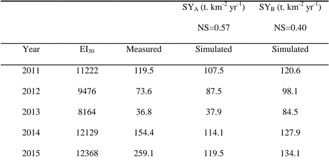
(kg h MJ-1 mm-1), LS2D is a parameter reflecting the slope steepness and length based on
147
the algorithms of Desmet and Govers (1996), and the slope factor LS2D is adjusted using a
148
two-dimensional routing algorithm (Van Oost et al., 2000) to account for rill, inter-rill and
149
gully erosion (Desmet et al., 1999), C is soil coverage factor (including biomass and mulch
150
depending on soil use and management; (Renard et al, 1997), and P the (optional) soil
151
conservation factor.
152
Two rainfall monitoring stations from the Water National Agency (ANA) located
153
within the catchment(Fig. 1) with 50-yr records were used to estimate the R factor.
154
Erosivity was calculated with an equation using monthly and annual rainfall developed by
155
Cassol et al., (2007) for Southern Brazil.
156
Erodibility (factor K) was calculated using equations developed by Roloff & Denardin
157
(1994) for Brazilian soils. The physical and chemical parameters required to apply the
158
equations were measured in the different soil classes, and their spatial distribution was
159
estimated from the soil map. Acrisols showed the highest susceptibility to erosion with a K
Page 8
value of 0.03756, followed by Nitosols with a K of 0.01752. Oxisols, which cover
161
approximately 80% of the catchment surface area, were associated with values ranging
162
from 0.01155 to 0.01590. This demonstrates that most soils of the catchment show a very
163
high aggregate stability. The physical parameters used to calculate the K factor were the
164
soil texture, considering the grain size (0.02 mm), silt (0.02 - 0.005 mm) and fine sand (0.2
165
- 0.005 mm g g -1 ) as well as the percentage of permeability of each soil type (mm h-1). As
166
for the chemical parameters, the iron (Fe2O3) and aluminum (Al2O3) oxides (g kg-1) were
167
used for each soil class; temporal variability in the K factor values was not considered,
168
because the paramethers involved in determining the K-factor had not been altered.In
169
order to calculate the topographic factor (LS2D), the Digital Elevation Model (DEM) was
170
created by interpolating between the contour lines of digital topographic maps with a 20-m
171
resolution. The LS2D factor was calculated based on the algorithm proposed by Desmet and
172
Govers (1996). Considers that gully erosion is not dominant in the Conceição catchment.
173
Only few ephemeral gullies occur in the area. Gully erosion can be found in some
174
locations, but we still do not know how much it contributes to total sediment yield (SY).
175
Aimming to represent such processes, the Watem Sedem modell uses the LS factor to
176
represent the sediment transport capacity.
177
In order to represent the transport capacity the modell uses the logarithm of Desmet
178
et al. (1999) and Desmet and Govers (1996), which describes the LS factor and associates
179
the gullies process. The modell incorporates different criteria and uses topographic
180
attributes to indicate the location of the gullies' starting points, flow direction,
181
characteristics of soil surface, vegetation cover, slope gradient and length.
182
Accordingly, the original transport capacity equation was used (Van Rompaey et
183
al., 2001), which allows the model to represent the connections directly through channels
184
with flow concentration preferential pathways (thalwegs) connecting water and sediment
Page 9
flows on hillslopes with the rivers (Verstraeten et al., 2006) and / or interrupt the flows
186
with either natural or mechanical barriers. The C-factor was determined using the
187
methodology described by (Renard et al., 1997).Crop rotation (C-factor) aims to reduce
188
the direct impact of rainfall events on the soil surface. Annual values of C-factor were
189
attributed according to the land use (cropland, pasture and forest). The spatial distribution
190
of the C-factor for the catchment fields was based on of the analysis of satellite images and
191
field surveys (Table 1). In addition to the BAU conditions (Chigh), an alternative scenario
192
(Clow) was constructed including an increase of crop rotations, with the planting of turnip
193
(winter) and maize (summer) in addition to the traditional soybean and wheat crops. This
194
study seeks to understand the effect of current conservation measures adopted by farmers,
195
and the impact of crop rotation on soil loss and the connectivity of sediments to
196
rivers.Table 1 - Values for the soil cover factor (C) simulated for the Conceição River
197
Catchment.
198
* Business-as-usual; C : Factor C, Cs : Soil Cover, Cc : Cover by canopy, PU : Prior
199
land use, Rs : surface roughness.
200
The P factor corresponds to the efficiency of conservation measures implemented
201
in the catchment. A value of 1 represents the worst case scenario with the least efficiency
202
(tillage). Currently, no-tillage is the only conservation measure implemented in the
203
catchment. Accordingly, a mean value of 0.8, which corresponds to a 20% water retention
204
efficiency, was attributed to the P factor for the entire catchment. In the study area, crops
205
are usually sown in the direction parallel to the longest field boundary (i.e. typically
206
perpendicular to the contour lines). In order to quantify the potential impact of crop
207
levelling in the catchment, the angle between the contour lines and the sowing rows was
208
measured (mean angle of 45°). According to the equation provided by (Renard et al, 1997),
Page 10
the sowing efficiency was estimated to 0.20, which will affect the value of P for each pixel
210
depending on the local slope.
211
Eq. (1) estimates the amount of sediment generated, and consequently, transferred
212
to lower sections of the hillslope until it reaches the permanent drainage network. The
213
amount of sediments transported by surface flow depends on the soil transport capacity
214
(Tc) (Eq. 2), which is controlled by the physiographic factors of the cell considered (Van
215
Rompaey et al., 2001). Tc is the maximum amount of soil that can be transported from a
216
given pixel per length unit to the adjacent pixel, assuming that the transport capacity is
217
proportional to the potential of gully erosion.
218 219
Where: Tc is the transport capacity expressed as (kg m-1 yr-1), ktc is the coefficient of
220
transport capacity, expressed in m; R, K and LS2D are RUSLE factors (Renard et al, 1997),
221
and Sg is the steepness of the slope (m m-1).
222
The transport capacity coefficient Ktc (m) describes the proportionality between the
223
potential for rill erosion and the transport capacity. It can be interpreted as the theoretical
224
upslope distance that is needed to produce sufficient sediment to reach the transport
225
capacity of the cell considered, assuming a uniform slope and runoff discharge
226
(Verstraeten et al., 2006).
227
WATEM/SEDEM employs a routing algorithm to transfer the eroded sediment
228
from the source to the river network (Desmet and Govers, 1996; Van Oost et al., 2000).
229
This algorithm was improved by (Haregeweyn et al., 2013). The distribution between soil
230
erosion, transport and deposition processes is controlled by the values of E (Erosion) and
231
Tc (transport capacity): when E> Tc, deposition will occur, whereas there will be sediment
232
transfer when E <Tc.
233
2.4 Model calibration and scenarios
Page 11
The model was calibrated based on sediment yields measured from 2011 to 2015.
235
The calibration parameters were the transport coefficients KtcLow and Ktchigh obtained by
236
minimizing the difference between simulated and measured values.The parameters of plot
237
efficiency (Ptef) in cropland, forests and pastures were 20, 90 and 60, respectively. The
238
parcel connectivity parameter (PC) was set to 20 for cropland and to 60 for forest and
239
pasture. The method described by (Moriasi et al., 2007) was used to quantify the statistical
240
efficiency of the WaTEM/SEDEM model to simulate the sediment yield.
241
Following the calibration of the model for the BAU conditions (factor P with 20%
242
efficiency), four alternative scenarios including different combinations of conservation
243
measures were modelled, with two sets of rainfall conditions (a dry year [Rlow] with 1458
244
mm, corresponding to the situation observed in 2013; vs. a wet year [Rhigh] with 2251 mm,
245
corresponding to 2014) to quantify their respective impact on erosion, deposition and
246
sediment yield.
247
Two physical criteria were used to design the conservation scenarios: they had not
248
to be implemented yet by the farmers in the catchment and they had to limit sediment
249
connectivity within the catchment.The selected scenarios incorporate the vegetative and
250
mechanical practices for erosion control. The chosen vegetative practices (different
251
rotations) involve economic criteria, since that is the criteria most often used when
252
farmers implement parcial conservation measures. With this criteria in mind, there are
253
more effective practices that could be implemented maintaining their medium to long-term
254
financial expectations. The mechanical practices (terraces, areas of permanent forest
255
preservation) were chosen considering their ability to control surface runoff and increase
256
soil surface friction, thus, reducing the speed of the water flow. since such measures are
257
currently not present in the selected catchment. Five scenarios were modelled including a
Page 12
business-as-usual (BAU) scenario representing current land use and management
259
conditions and four alternative soil conservation scenarios (Table 2):
260
Table 2: Scenarios modelled in the Conceição River catchment.
261
(BAU) business-as-usual scenario: Chigh; Scenario I: Clow; Scenario II: Clow + CL +
262
T; Scenario III: Clow + CL + T + APP; Scenario IV: Clow + APP. Where: CL : crop
263
levelling; T: terracing; APP : areas of permanent forest preservation.
264
It should be noted that the Brazilian Forestry Code legislation determines that
265
certain zones in the catchment should be considered as areas of permanent forest
266
preservation (APP) because of their importance for protecting the environment and the
267
quality of water resources. These include areas adjacent to rivers or natural and artificial
268
reservoirs, and hillslope sections with slope angles steeper than 45°. Removal of the
269
vegetation in these areas is only allowed in certain occasions (e.g. social interest), provided
270
previous authorization is obtained from the appropriate environmental agencies.
271
3. Results
272
3. 1 Hydrology and sediment yield
273
Figure 2 shows the rainfall variability and erosivity from 2011 to 2015. The
274
monitoring period was heterogeneous, with long periods of drought in 2012 and periods of
275
concentrated rainfall in 2011, 2014 and 2015. In contrast, 2013 was characterized by a
276
rainfall amount close to the long-term average, despite the occurrence of rainfall events of
277
low-to-medium intensity and storms of extreme magnitude. The high intensity rainfall
278
observed in November and December 2015 is attributed to the El Niño phenomenon
279
(Marengo et al., 2009). This rainfall distribution affected the hydrological conditions in the
280
river and the resulting sediment fluxes. The highest sediment fluxes were observed during
281
the years characterized by the highest water discharges (Table 3).
Page 13
Figure 2 - Monthly rainfall and erosivity data of the Conceição River catchment for
283
the monitoring period (2011to 2015).
284
Table 3 - Representation of hydro-sedimentological variables of the Conceição River
285
catchment for the monitoring period (2011to 2015).
286
R: rainfall (mm); SSD: suspended sediment discharge; Q: Flow rate (m³ s-1), SY:
287
Sediment yield (t. km-2)); EI30 (MJ mm ha-1 h-1).
288
In addition to this inter-annual variability, water flow (Q) and sediment yields (SY)
289
exhibited large seasonal variations controlled by rainfall distribution (R) and agricultural
290
practices affecting the sensitivity of soils to runoff and erosion (Figure 3).
291
The large impact of rainfall events occurring in spring on the increase of water
292
discharges, runoff and sediment yield is demonstrated.
293
Figure 3 - Monthly averages (2011-2015) of sediment yield (SY), Flow (Q), rainfall (R)
294
for the Conceição River catchment.
295
3.2 Model efficiency analysis
296
The model and the transport capacity coefficient (Ktc) were initially calibrated
297
considering the entire dataset covering the five years of monitoring (SYA - Table 4). The
298
performance of the model measured by the efficiency index (SE- Statistical Efficiency)
299
was 40%. When excluding 2015 from the calibration data (SYB – Table 4), the efficiency
300
of the model increased by 20%, to 60%. This is likely due to the atypical climate
301
conditions observed in 2015, with the occurrence of several extreme events that likely
302
modified the transport capacity and mobilized distinct sediment sources (e.g. channel
303
banks, roads).
304
The correspondence between the measured and the simulated mean annual SY
305
(t.km-2 year-1) for a 5-year period using the WaTEM/SEDEM model is shown in Figure 4.
Page 14
Figure 4 - Performance of the WaTEM / SEDEM model in predicting sediment
307
yield (SY) for Conceição River.
308
When restricting the calibration period to 2011–2014, the optimized PC and
309
KTc_Low values were 60 and 0.12 for forests and pastures, and 20 and 0.36 for cropland,
310
respectively. The results of the simulations performed after the calibration are presented in
311
Table 4.
312
Table 4 - Representation of calibration from sediment yield at the monitoring station
313
and efficiency of the model.
314
Where: EI30 : Erosivity (MJ mm ha-1h-1), SY : Sediment yield (t.km-2): Sub index
315
A:four year database (from 2011 to 2014) and B : five year database (from 2011 to
316
2015).
317
3.3 Modelling alternative soil conservation scenarios
318
Sediment yields were simulated for the BAU conditions and the four alternative
319
land cover scenarios (Table 5). Scenario I simulating the implementation of crop rotation
320
with plants providing higher biomass densities to protect the soils reduced only erosion by
321
0.6% and sediment yield by 1% compared to the BAU scenario. Scenario II included crop
322
rotation as well as crop levelling and terracing, and reduced erosion by 358%, deposition
323
by 316% and sediment yield by 400%. Scenario III combined the conservation measures
324
implemented in scenario II and areas of permanent forest preservation. It was the most
325
effective, with a reduction of soil erosion by 378%, a decrease of sediment deposition by
326
274% and of sediment yield by 541%. Scenario IV combined the introduction of crop
327
rotation and permanent forest preservation areas and led to a decrease of only 6.8% in
328
erosion and of approximately 38% in sediment yield. Furthermore, this was the only
329
scenario associated with an increase of sediment deposition rates (14%).
Page 15
Table 5 - Results of erosion, sediment deposition and sediment yield estimated by the
331
WaTEM-SEDEM model for the different scenarios.
332
*data set from 2013, representative of a dry year with cumulative rainfall lower than
333
the long-term average (1458 mm);
334
**data set from 2014, representative of a wet year with cumulative rainfall above the
335
long-term average (2251 mm).
336
Overall, all simulated processes (erosion, deposition and sediment yield) were
337
33.9% higher under wet conditions (Rhigh) than under dry conditions (Rlow; Figure 5).
338
Figure 5 - Results of erosion, sediment deposition and sediment yield estimated
339
by the WaTEM-SEDEM model for the different scenarios simulated for Rlow and
340
Rhigh.
341
Figure 6 shows the spatial pattern of soil losses within the Conceição catchment,
342
illustrating the important role played by topography (including slope length, steepness and
343
curvature) to explain spatial variations of erosion.The interactions of the LS factor with
344
the other RUSLE parameters are determined automatically by the WaTEM/SEDEM
345
model.The topographic attributes (LS) also consider the interactions of the soil surface and
346
the vegetation cover (C-factor), as well as the flow direction, which can be altered and/or
347
controlled through the mechanical practices (P-factor). Based on criterion such as
348
interventions in C factor values with increased plant biomass as well as factor P. Values for
349
both C and P factors were used to verify the responses of the different levels of
350
intervention on the values of soil losses and river connectivity.
351
Large volumes of runoff and sediment may accumulate on the long convex
352
hillslopes of the catchment and concentrate when reaching the river system, which exposes
353
the lower third section of the slopes to higher erosion rates.Figure 6 - Spatial
354
representation of the erosion of the Conceição River catchment, according to the
Page 16
proposed scenarios: a):BAU: Chigh; B) Scenario I: Clow; C) Scenario II: Clow + CL + T;
356
D) Scenario III: Clow + CL + T + APP; E) Scenario IV: Clow + APP. Where: CL: crop
357
levelling; T: terracing; APP: areas of permanent forest preservation.
358
4. Discussion
359
4.1 Effectiveness of land cover scenarios to control soil erosion and sediment yield
360
A comparison of the results of all scenarios for both dry (Rlow) and wet (Rhigh)
361
conditions shows that scenario III is the most efficient in reducing the intensity of erosion
362
and sediment transfer processes. Among the measures included in this scenario, the
363
mechanical conservation measures (simulated in both scenarios II and III) are likely the
364
most effective as they lead to a three-fold decrease of soil loss and sediment yields. In
365
contrast, the introduction of a crop rotation alone (scenario I) does not provide significant
366
erosion control. Results comparable to those obtained for scenario II are simulated for
367
scenario III, including the implementation of APPs. The contribution of APPs alone,
368
without the association with mechanical measures, is simulated in scenario IV. The model
369
indicates the relatively low efficiency of this scenario to control erosion processes,
370
although it is the single set of conditions leading to a 14% increase in sediment deposition.
371
This result illustrates the reduction of sediment velocity and the greater retention of
372
sediment in the APPs. Previous studies demonstrated that riparian vegetation leads to a
373
drastic decrease of sediment delivery (Cooper et al., 1987; Verstraeten et al., 2006).
374
However, when applied without the implementation of additional measures to control
375
sediment production at the source, this strategy is found not to be efficient in controlling
376
erosion (less than 10% reduction when compared to the BAU scenario), as cropland was
377
shown to provide the main source of sediment in this catchment (Tiecher et al., 2014).
378
4.2 Impact of land cover scenarios on sediment connectivity
Page 17
Several scenarios have a clear impact on sediment connectivity, by affecting the
380
link between the sediment produced on the hillslopes and the material transiting the river
381
(Croke et al., 2005). In particular, the implementation of forest preservation areas in zones
382
of flow convergence or in the alluvial plains decreases sediment connectivity
(Quiñonero-383
Rubio et al., 2014). For instance, a change in land use in targeted zones through the
384
reforestation in fragile areas (Rompaey and Govers, 2002) may have an immediate impact
385
and reduce gross erosion and sediment connectivity (Alatorre et al., 2012). When
386
implementing APPs in the catchment, the model simulated a 38% reduction in sediment
387
yield and a 14% increase in sediment deposits (fig. 5), although it had limited impact on
388
gross erosion. The large heterogeneities in sediment connectivity simulated in the
389
catchment may reflect the spatial pattern of the conservation measures implemented in the
390
region (e.g. location of terraces; Fig. -6) or the intensity of rainfall events. Sediment
391
connectivity varies according to the intensity of the monthly and annual rainfall events.
392
Acccordingly, sediment flows are heterogeneous over time. As found in other regions of
393
the world, the highest sediment connectivity between hillslopes and rivers is achieved
394
during the most intense events (e.g. during typhoons in Asia) (Chartin et al., 2016). The
395
lower efficiency of the WaTEM/SEDEM model during the most intense events may be
396
explained by the fact that roads and channels were not taken into account by the model,
397
and their inclusion in the future should improve the quality of the model results during
398
these intense storms.
399
4.3 Improvement of soil conservation in Southern Brazil
400
The scenario simulations demonstrated that there is a need to combine erosion
401
control measures on the cultivated fields (e.g. implementation of crop rotations, increase of
402
the vegetation cover of the soils) to reduce soil loss at the source, with additional measures
403
reducing sediment connectivity between hillslopes and rivers. The catchment is
Page 18
characterized by the intensive soybean/wheat monoculture, which limits the diversity of
405
crops characterized by contrasting growing stages. In Europe, the variety of crops found on
406
a hillslope may create heterogeneous landscape mosaics, with bare soils producing
407
runoff/sediment and zones densely covered by vegetation that may reinfiltrate runoff and
408
trap sediment (Evrard et al., 2007; Souchère et al., 2005). The main soil characteristics
409
controlling runoff and sediment production at the field scale (i.e., soil cover by vegetation,
410
soil roughness, crusting stage) generally vary throughout the year, as a result of plant
411
growth, weather conditions and farming practices (Cerdan et al., 2002; Evrard et al.,
412
2008a). In southern Brazil, the most sensitive periods for runoff and erosion are winter and
413
spring, during the plant initial growth stage or after the harvest, when rainfall is the most
414
abundant (Figure 3). The modelled scenarios showed that soil cover by vegetation is not
415
sufficient during these periods to control erosion (Figure 5; Table 5), and it should be
416
increased to better protect the soils and further limit runoff/sediment production (Reicosky,
417
2015).
418
In addition, measures aimed to reducing sediment connectivity will act as a
419
physical barrier and prevent the sediment from reaching the water bodies when they are
420
located on the main runoff/sediment flow pathways (Boix-Fayos et al., 2008). Specific
421
plantation patterns (e.g. crop levelling, contour ploughing) can reduce sediment
422
connectivity (Karlen et al., 2009). Species such as elephant (Pennisetum purpureum),
423
vetiver (Chrysopogon zizanioides) and lemon grasses (Cymbopogon citratus) were shown
424
to provide effective sediment retention traps when planted in thalwegs or in concentrated
425
flow areas (Fiener and Auerswald, 2003; Verstraeten et al., 2002). An alternative to the
426
planting of specific vegetation species could be the installation of small earthen dams in
427
the thalwegs in order to slow down runoff and trap sediment. In Europe, these
428
measurements were shown to reduce sediment yield by 90% (Evrard et al., 2008a; Evrard
Page 19
et al., 2008b). Importantly, there is a need to coordinate the implementation of these
430
control measures, both at the source and on the main flow pathways, at the catchment scale
431
in order to increase their effectiveness, as it was illustrated in regions of Northwestern
432
Europe where this type of measures was monitored in pilot areas (Evrard et al., 2010).
433
4.4 Perspectives for future research
434
Despite the widespread use of no-till in Southern Brazil, soil erosion and sediment
435
transfer remain excessive. Additional measures should be taken to improve this situation,
436
through the implementation of mechanical conservation measures, the increase of biomass
437
cover density of the soil, and the decrease of traffic of agricultural machinery to increase
438
the soil infiltration rates and sediment trapping (Denardin et al., 2008).
439
A previous modelling study compared the impact of applying conventional tillage
440
vs. no-till in a 20-km² catchment of Southern Brazil characterized by similar soil
441
characteristics, relief and land use as the study site investigated by the current research
442
(Castro et al., 1999). These authors showed that the runoff coefficient was higher when
443
applying no-till alone (7.7%) than when combining the use of conventional tillage and
444
terraces (5.8%). Other studies used the sediment fingerprinting technique to quantify the
445
sources supplying sediment to river systems of Southern Brazil. They showed that soils
446
found in lower parts of the catchment, cultivated with conventional practices on steep
447
slopes, were the main source of sediment to the Guaporé River network (Le Gall et al.,
448
2017). In contrast, soils found in upper parts of the catchment, cultivated with soybean
449
under direct sowing, deposited in ponds or in riparian areas before reaching the outlet. This
450
demonstrates the effectiveness of a strategy combining measures at the source and physical
451
barriers along the main flow pathways in the catchment.
452
Although models can provide powerful helping-decision tools for environmental
453
management, their use depends on the availability of large input datasets for calibration
Page 20
(Tab.4). In the future, other soil erosion models such as STREAM (Cerdan et al., 2002),
455
APEX (Williams et al., 2008), or SWAT (Williams and Arnold, 1997) could be used to
456
investigate the impact of climate change on the effectiveness of conservation measures.
457
The magnitude and the frequency of heavy storms are expected to increase, which should
458
modify the production and the transfer of sediment across the landscape. The analysis of
459
sediment (dis)connectivity impact by these changes in interaction with the implementation
460
of contrasted conservation scenarios could usefully be tested in order to protect soil and
461
water resources and to allow their sustainable use for agriculture production.
462
5 Conclusions
463
Sediment fluxes were monitored from 2011 to 2015 in the Conceição catchment,
464
representative of cultivated environments under no-till in Southern Brazil. Very high
465
sediment yields, characterized by strong inter-annual variations (37–259 t km-2 yr-1), were
466
measured at the catchment outlet. These results illustrate that the use of no-tillage alone is
467
not sufficient to control soil erosion in this region. The WaTEM/SEDEM erosion model
468
was calibrated and validated with the unique dataset obtained in Conceição, and was
469
subsequently used to simulate contrasted land cover scenarios in order to propose a
470
sustainable use of soil resources in this intensively cultivated region.
471
The combination of direct sowing with measures recommended by the conservation
472
agriculture principles (e.g. increase in biomass cover of the soil, crop rotation, physical
473
barriers) was shown to lead to a 3-to-5 fold reduction of soil loss and sediment yields in
474
this region. Model simulations demonstrated in particular the need to implement
475
mechanical measures and to preserve riparian forests to slow down runoff and trap
476
sediment. This integrated soil conservation strategy should be tested in these environments
477
of Southern Brazil, in order to promote sustainable farming practices and to prevent the
478
further degradation of water quality.
Page 21
Acknowledgements
480
The research benefited from the support of the CAPES-COFECUB project no
481
Te870-15.
482
6 References
483
Alatorre, L.C., Beguería, S., Lana-Renault, N., Navas, A., García-Ruiz, J.M., 2012. Soil
484
erosion and sediment delivery in a mountain catchment under scenarios of land use
485
change using a spatially distributed numerical model. Hydrol. Earth Syst. Sci. 16,
486
1321–1334. doi:10.5194/hess-16-1321-2012
487
Bertol, I., Cogo, N.P., Schick, J., Gudagnin, J.C., Amaral, A.J., 2007. Aspectos financeiros
488
relacionados às perdas de nutrientes por erosão hídrica em diferentes sistemas de
489
manejo do solo. Rev. Bras. Ciência do Solo 31, 133–142.
doi:10.1590/S0100-490
06832007000100014
491
Bezak, N., Rusjan, S., Petan, S., Sodnik, J., Mikoš, M., 2015. Estimation of soil loss by the
492
WATEM/SEDEM model using an automatic parameter estimation procedure.
493
Environ. Earth Sci. doi:10.1007/s12665-015-4534-0
494
Boix-Fayos, C., De Vente, J., Martínez-Mena, M., Barberá, G.G., Castillo, V., 2008. The
495
impact of land use change and check-dams on catchment sediment yield 22, 4922–
496
4935. doi:10.1002/hyp.7115
497
Bolliger, A., Magid, J., Amado, J.C.T., Skóra Neto, F., Ribeiro, M. de F. dos S., Calegari,
498
A., Ralisch, R., de Neergaard, A., 2006. Taking Stock of the Brazilian “Zero‐Till
499
Revolution”: A Review of Landmark Research and Farmers’ Practice. Adv. Agron.
500
91, 47–110. doi:10.1016/S0065-2113(06)91002-5
501
Cassol, E.A., Martins, D., Luiz, F., Eltz, F., Lima, V.S. De, 2007. Erosividade e padroes
502
hidrologicos das chuvas de Ijui ( RS ) no periodo de 1963 a 1993 Erosivity and
503
hydrological patterns of Ijui ( RS , Brazil ) rainfalls in the period of 1963 to 1993.
Page 22
Rev. Bras. Agrometeorol. 15, 220–231.
505
Castro, N.M.D.R., Auzet, A.-V., Chevallier, P., Leprun, J.-C., 1999. Land use change
506
effects on runo and erosion from plot to catchment scale on the basaltic plateau of
507
Southern Brazil. Hydrol. Process. 13, 1621–1628.
508
Cerdan, O., Souchère, V., Lecomte, V., Couturier, A., Le Bissonnais, Y., 2002.
509
Incorporating soil surface crusting processes in an expert-based runoff model: Sealing
510
and Transfer by Runoff and Erosion related to Agricultural Management. CATENA
511
46, 189–205. doi:10.1016/S0341-8162(01)00166-7
512
Chartin, C., Evrard, O., Laceby, J.P., Onda, Y., Ottlé, C., Lefèvre, I., Cerdan, O., 2016.
513
The impact of typhoons on sediment connectivity: Lessons learnt from contaminated
514
coastal catchments of Fukushima Prefecture (Japan). Earth Surface Processes and
515
Landforms. DOI: 10.1002/esp.4056.
516
Cooper, J.R., Gilliam, J.W., Daniels, R.B., Robarge, W.P., 1987. Riparian areas as filters
517
for agricultural sediment. Soil Sci. Soc. Am. J.
518
Croke, J., Mockler, S., Fogarty, P., Takken, I., 2005. Sediment concentration changes in
519
runoff pathways from a forest road network and the resultant spatial pattern of
520
catchment connectivity 68, 257–268. doi:10.1016/j.geomorph.2004.11.020
521
de Moor, J.J.W., Verstraeten, G., 2008. Alluvial and colluvial sediment storage in the Geul
522
River catchment (The Netherlands) — Combining field and modelling data to
523
construct a Late Holocene sediment budget. Geomorphology 95, 487–503.
524
doi:10.1016/j.geomorph.2007.07.012
525
Denardin, J.E., Kochhann, R.A., Faganello, A., Sattler, A., Manhago, D.D., 2008. “Vertical
526
mulching” como prática conservacionista para manejo de enxurrada em sistema
527
plantio direto. Rev. Bras. Ciência do Solo 32, 2847–2852.
doi:10.1590/S0100-528
06832008000700031
Page 23
Derpsch, R., Franzluebbers, A.J., Duiker, S.W., Reicosky, D.C., Koeller, K., Friedrich, T.,
530
Sturny, W.G., Sá, J.C.M., Weiss, K., 2014. Why do we need to standardize no-tillage
531
research? Soil Tillage Res. doi:10.1016/j.still.2013.10.002
532
Desmet, P.J.J., Govers, G., 1996. A GIS procedure for automatically calculating the USLE
533
LS factor on topographically complex landscape units. J. Soil Water Conserv. 51,
534
427–433.
535
Desmet, P.J.J., Poesen, J., Govers, G., Vandaele, K., 1999. Importance of slope gradient
536
and contributing area for optimal prediction of the initiation and trajectory of
537
ephemeral gullies.
538
Evrard, O., Heitz, C., Liégeois, M., Boardman, J., Vandaele, K., Auzet, A.-V., van
539
Wesemael, B., 2010. A comparison of management approaches to control muddy
540
floods in central Belgium, northern France and southern England. L. Degrad. Dev. 21,
541
322–335. doi:10.1002/ldr.1006
542
Evrard, O., Persoons, E., Vandaele, K., Wesemael, B. Van, 2007. Effectiveness of erosion
543
mitigation measures to prevent muddy floods : A case study in the Belgian loam belt
544
118, 149–158. doi:10.1016/j.agee.2006.02.019
545
Evrard, O., Vandaele, K., van Wesemael, B., Bielders, C.L., 2008a. A grassed waterway
546
and earthen dams to control muddy floods from a cultivated catchment of the Belgian
547
loess belt. Geomorphology 100, 419–428. doi:10.1016/j.geomorph.2008.01.010
548
Evrard, O., Vandaele, K., Wesemael, B. Van, Bielders, C.L., 2008b. A grassed waterway
549
and earthen dams to control muddy floods from a cultivated catchment of the Belgian
550
loess belt 100, 419–428. doi:10.1016/j.geomorph.2008.01.010
551
Fiener, P., Auerswald, K., 2003. Effectiveness of Grassed Waterways in Reducing Runoff
552
and Sediment Delivery from Agricultural Watersheds. J. Environ. Qual. 32, 927.
553
doi:10.2134/jeq2003.9270
Page 24
Foster, G.R., Toy, T.E., Renard, K.G., 2003. Comparison of the USLE, RUSLE1.06c, and
555
RUSLE2 for Application to Highly Disturbed Lands. USDA-ARS 154–160.
556
Fu, B.J., Zhao, W.W., Chen, L.D., Zhang, Q.J., Lü, Y.H., Gulinck, H., Poesen, J., 2005.
557
Assessment of soil erosion at large watershed scale using RUSLE and GIS: A case
558
study in the Loess Plateau of China. L. Degrad. Dev. doi:10.1002/ldr.646
559
Le Gall, M., Evrard, O., Dapoigny, A., Tiecher, T., Zafar, M., Paolo, J., Minella, G.,
560
Laceby, J.P., Ayrault, S., 2017. Tracing sediment sources in a subtropical agricultural
561
catchment of southern Brazil cultivated with conventional and conservation farming
562
practices.L. Degrad. Dev.DOI: 10.1002/ldr.2662
563
Gómez, J.A., Battany, M., Renschler, C.S., Fereres, E., 2003. Evaluating the impact of soil
564
management on soil loss in olive orchards. Soil Use Manag. 19, 127–134.
565
doi:10.1111/j.1475-2743.2003.tb00292.x
566
Haregeweyn, N., Poesen, J., Verstraeten, G., Govers, G., Vente, J.D.E., Nyssen, J.,
567
Deckers, J., Moeyersons, J., 2013. Assessing the performance of a spatially
568
distributed soil erosion and sediment delivery model ( WaTEM / SEDEM ) IN 204,
569
188–204.
570
Horowitz, A.J., Elrick, K.A., Smith, J.J., Stephens, V.C., 2014. The effects of Hurricane
571
Irene and Tropical Storm Lee on the bed sediment geochemistry of U.S. Atlantic
572
coastal rivers. Hydrol. Process. 28, 1250–1259. doi:10.1002/hyp.9635
573
Karlen, D.L., Dinnes, D.L., Tomer, M.D., Meek, D.W., Cambardella, C.A., Moorman,
574
T.B., 2009. Is No-Tillage Enough ? A Field-Scale Watershed Assessment of
575
Conservation Effects 7, 1–24.
576
Keesstra, S.D., van Dam, O., Verstraeten, G., van Huissteden, J., 2009. Changing sediment
577
dynamics due to natural reforestation in the Dragonja catchment, SW Slovenia.
578
CATENA 78, 60–71. doi:10.1016/j.catena.2009.02.021
Page 25
Kinnell, P.I.A., 2010. Event soil loss, runoff and the Universal Soil Loss Equation family
580
of models: A review. J. Hydrol. 385, 384–397. doi:10.1016/j.jhydrol.2010.01.024
581
Knapen, A., Poesen, J., Govers, G., Gyssels, G., Nachtergaele, J., 2007. Resistance of soils
582
to concentrated flow erosion: A review. Earth-Science Rev. 80, 75–109.
583
doi:10.1016/j.earscirev.2006.08.001
584
Lal, R., 2007. Constraints to adopting no-till farming in developing countries. Soil Tillage
585
Res. 94, 1–3. doi:10.1016/j.still.2007.02.002
586
Lal, R., Delgado, J.A., Gulliford, J., Nielsen, D., Rice, C.W., Pelt, R.S. Van, 2012. extreme
587
events 67, 162–166. doi:10.2489/jswc.67.6.162A
588
Marengo, J.A., Jones, R., Alves, L.M., Valverde, M.C., 2009. Future change of
589
temperature and precipitation extremes in South America as derived from the PRECIS
590
regional climate modeling system 2255, 2241–2255. doi:10.1002/joc
591
Merten, G.H., Horowitz, A., Clarke, R., Minella, J., Pickbrenner, K., Pinto, M., 2006.
592
Considerações sobre a utilização da curva-chave para determinação de fluxo de
593
sedimentos - Quantificação das incertezas nas estimativas do fluxo de sedimentos em
594
suspensão, gerados a partir de uma curva-chave.
595
Minella, J.P.G., Merten, G.H., Reichert, J.M., Clarke, R.T., 2008. Estimating suspended
596
sediment concentrations from turbidity measurements and the calibration problem.
597
Hydrol. Process. 22, 1819–1830. doi:10.1002/hyp.6763
598
Montgomery, D.R., 2007. Soil erosion and agricultural sustainability. Proc. Natl. Acad.
599
Sci. U. S. A. 104, 13268–72. doi:10.1073/pnas.0611508104
600
Moriasi, D.N., Arnold, J.G., Liew, M.W. Van, Bingner, R.L., Harmel, R.D., Veith, T.L.,
601
2007. M e g s q a w s 50, 885–900.
602
Nearing, M.A., Govers, G., Norton, L.D., 1999. Variability in Soil Erosion Data from
603
Replicated Plots. Soil Sci. Soc. Am. J. 63, 1829. doi:10.2136/sssaj1999.6361829x
Page 26
Nearing, M., Pruski, F.F., O’Neal, M.R., 2004. Expected climate change impacts on soil
605
erosion rates: A review. J. Soil Water Conserv. 59, 43–50.
606
Notebaert, B., Verstraeten, G., Ward, P., Renssen, H., Rompaey, A. Van, 2011.
607
Geomorphology Modeling the sensitivity of sediment and water runoff dynamics to
608
Holocene climate and land use changes at the catchment scale 126, 18–31.
609
doi:10.1016/j.geomorph.2010.08.016
610
Okoro, B.C., Ibearugbulem, 2013. Gully Erosion Control along NWORIE River in Owerri,
611
\nImo State-A Deterministic Model Approach. Ijmer 3, 1774–1782.
612
Poesen, J., 2011. Challenges in gully erosion research 17, 5–9.
613
Porterfield, 1977. Computation of fluvial-sediment discharge.
614
Quiñonero-Rubio, J.M., Nadeu, E., Boix-Fayos, C., de Vente, J., 2014. Evaluation of the
615
Effectiveness of Forest Restoration and Check-Dams to Reduce Catchment Sediment
616
Yield. L. Degrad. Dev. 27, 1018–1031. doi:10.1002/ldr.2331
617
Reicosky, D.C., 2015. Conservation tillage is not conservation agriculture. J. Soil Water
618
Conserv. 70, 103A–108A. doi:10.2489/jswc.70.5.103A
619
Renard et al, 1997. Predicting Soil Erosion by Water: A Guide to Conservation Planning
620
with the Revised Universal Soil Loss Equation (RUSLE), 703rd ed. Washington, DC.
621
Roloff, G & Denardin, JE (1994). Estimativa simplificada da erodibilidade do solo. In.
622
Reunião Brasileira de Manejo e Conservação do Solo e da Água, Florianópolis. 10º,
623
Anais. Florianópolis: Sociedade Brasileira de Ciência do Solo. p.150-151.
624
Rompaey, A. Van, Bazzoffi, P., Jones, R.J.A., Montanarella, L., 2005. Modeling sediment
625
yields in Italian catchments. Geomorphology 65, 157–169.
626
doi:10.1016/j.geomorph.2004.08.006
627
Rompaey, A.J.J. Van, Govers, G., n.d. Data quality and model complexity for regional
628
scale soil erosion prediction. Int. J. Geogr. Inf. Sci. 16, 663–680.
Page 27
Shreve, E.A., Downs, A.C., 2005. Quality-Assurance Plan for the Analysis of Fluvial
630
Sediment by the U.S. Geological Survey Kentucky Water Science Center Sediment
631
Laboratory.
632
Souza, C.M. de; Pires, F.R.; Partelli, F.L.; Assis, R.L. de Adubação verde e rotação de
633
culturas. Viçosa: Ed. UFV, 2012.108p.
634
Souchère, V., Cerdan, O., Dubreuil, N., Le Bissonnais, Y., King, C., 2005. Modelling the
635
impact of agri-environmental scenarios on runoff in a cultivated catchment
636
(Normandy, France). CATENA 61, 229–240. doi:10.1016/j.catena.2005.03.010
637
Terranova, O., Antronico, L., Coscarelli, R., Iaquinta, P., 2009. Soil erosion risk scenarios
638
in the Mediterranean environment using RUSLE and GIS: An application model for
639
Calabria (southern Italy). Geomorphology 112, 228–245.
640
doi:10.1016/j.geomorph.2009.06.009
641
Tiecher, T., Paolo, J., Minella, G., Miguel, P., Rasche, J.W., Pellegrini, A., Capoane, V.,
642
Ciotti, L.H., Luiz, G., 2014. Contribuição das fontes de sedimentos em uma bacia
643
hidrográfica agrícola sob plantio direto. 639–649.
644
Van Oost, K., Govers, G., Desmet, P., 2000. Evaluating the effects of changes in landscape
645
structure on soil erosion by water and tillage. Landsc. Ecol.
646
doi:10.1023/A:1008198215674
647
Van Rompaey, A.J.J., Verstraeten, G., Van Oost, K., Govers, G., Poesen, J., 2001.
648
Modelling mean annual sediment yield using a distributed approach. Earth Surf.
649
Process. Landforms. doi:10.1002/esp.275
650
Vente, J. De, Poesen, J., Verstraeten, G., 2008. Spatially distributed modelling of soil
651
erosion and sediment yield at regional scales in Spain 60, 393–415.
652
doi:10.1016/j.gloplacha.2007.05.002
653
Verstraeten, G., Oost, K. Van, Rompaey, A. Van, Poesen, J., Govers, G., 2002. Evaluating
Page 28
an integrated approach to catchment management to reduce soil loss and sediment
655
pollution through modelling. Soil Use Manag. 19, 386–394.
656
doi:10.1079/SUM2002150
657
Verstraeten, G., Poesen, J., Gillijns, K., Govers, G., 2006. The use of riparian vegetated
658
filter strips to reduce river sediment loads : an overestimated control measure ? 4267,
659
4259–4267. doi:10.1002/hyp.6155
660
Verstraeten, G., Rommens, T., Peeters, I., Poesen, J., Govers, G., Lang, A., 2009. A
661
temporarily changing Holocene sediment budget for a loess-covered catchment
662
(central Belgium). Geomorphology 108, 24–34. doi:10.1016/j.geomorph.2007.03.022
663
Wang, G., Hapuarachchi, P., Ishidaira, H., Kiem, A.S., Takeuchi, K., 2009. Estimation of
664
Soil Erosion and Sediment Yield During Individual Rainstorms at Catchment Scale.
665
Water Resour. Manag. 23, 1447–1465. doi:10.1007/s11269-008-9335-8
666
Williams, J.R., Arnold, J.G., 1997. A system of erosion-sediment yield models 11, 43–55.
667
Williams, J.R., Arnold, J.G., Kiniry, J.R., Gasaman, P.W., Green, C.H., 2008. History of
668
model development at Temple, Texas. Hydrol. Sci. J. 53, 948–960.
669
doi:10.1623/hysj.53.5.948
Table 1 - Values for the soil cover factor (C) simulated for the Conceição River Catchment.
C Cs Cc PU Rs
Chigh:Soybean/Fallow/Wheat/Soybean* 0.01794 0.122 0.576 0.236 0.980 Clow: Soybean/Turnip/Corn/Wheat 0.01260 0.106 0.529 0.170 0.969
* Business-as-usual; C = Factor C, Cs = Soil Cover, Cc = Cover by canopy, PU = Prior land use, Rs = surface roughness.
Table 2: Scenarios modelled in the Conceição River catchment.
Scenarios Factor C Additional conservation measure
BAU Chigh - - -
Scenario I Clow - - -
Scenario II Clow CL T -
Scenario III Clow CL T APP
Scenario IV Clow APP - -
(BAU) business-as-usual scenario: Chigh; Scenario I: Clow; Scenario II: Clow + CL + T; Scenario III: Clow + CL + T + APP; Scenario IV: Clow + APP. Where: CL: crop leveling; T: terracing; APP: areas of permanent forest preservation.
Table 3 - Representation of hydrossedimentological variables of the Conceição River catchment for the monitoring period (2011 to 2015).
R EI30 SSD(kg s-1) Q (m3 s-1) SY
Year Mean Maximum Mean Maximum
2011 2135 11222 2.58 423.5 24.2 998.3 119.5
2012 1632 9476 1.53 264.7 13.4 541.2 73.6
2013 1458 8164 0.73 57.5 18.6 488 36.8
2014 2251 12129 1.72 365.3 31.6 1442.8 154.4
2015 2470 12368 2.14 457.39 35.9 1051.7 259.1
R: rainfall (mm); SSD: suspended sediment discharge; Q: Flow rate (m³ s-1), SY: Sediment yield (t. km-2)); EI30 (MJ mm ha-1 h-1).
Table 4 - Representation of calibration from sediment yield at the monitoring station and efficiency of the model.
SYA (t. km-2 yr-1) NS=0.57
SYB (t. km-2 yr-1) NS=0.40
Year EI30 Measured Simulated Simulated
2011 11222 119.5 107.5 120.6
2012 9476 73.6 87.5 98.1
2013 8164 36.8 37.9 84.5
2014 12129 154.4 114.1 127.9
2015 12368 259.1 119.5 134.1
Where: EI30 : Erosivity (MJ mm ha-1h-1), SY : Sediment yield (t.km-2): Sub index A:four year database (from 2011 to 2014) and B : five year database (from 2011 to 2015). Table 4
Table 5 - Results of erosion, sediment deposition and sediment yield estimated by the WaTEM-SEDEM model for the different scenarios.
RLow * t. km-2 year-1
Model Conservation measures Erosion Deposition Sediment Yield
BAU Chigh 135.1 65.2 69.9
Scenario I Clow 134.3 (-0.5 %) 65.2 (0 %) 69.2 (-1%) Scenario II Clow +CL+T 29.6 (-356.4 %) 15.7 (-315.2%) 13.9 (-402.8) Scenario III Clow +CL+T+APP 28.3 (-377.3%) 17.4 (-274.7%) 10.9 (-541.2%) Scenario IV Clow +APP 126.5 (-6.7%) 75.8 (13.78%) 50.7 (-37.8%)
RHigh ** t. km-2 year-1
Model Conservation measures Erosion Deposition Sediment Yield
BAU Chigh 204.6 98.8 105.8
Scenario I Clow 203.4 (-0.6 %) 98.7 (-0.10%) 104.7 (-1.05 %) Scenario II Clow +CL+T 44.7 (-358 %) 23.7 (-316.8%) 21.0 (-403 %) Scenario III Clow +CL+T+APP 42.8 (-378 %) 26.4 (-274.2%) 16.5 (-541 %) Scenario IV Clow +APP 191.5 (-6.8%) 114.8 (13.9%) 76.7 (-37.9%) *data set from 2013, representative of a dry year with cumulative rainfall lower than the long-term average (1458 mm);
**data set from 2014, representative of a wet year with cumulative rainfall above the long-term average (2251 mm).
Figure Captions
Figure 1 - Location of the Conceição river catchment in Brazil.
Figure 2 - Monthly precipitation and rainfall erosivity in the Conceicao River catchment for the monitoring period (2011–2015).
Figure 3 - Monthly averages (2011–2015) of sediment yield (SY), river water discharge (Q), rainfall (R) for the Conceição River catchment.
Figure 4 - Performance the WaTEM/SEDEM model in predicting sediment yield (SY) for Conceição River.
Figure 5 - Results of erosion, sediment deposition and sediment yield estimated by the WaTEM-SEDEM model for the different scenarios simulated including those with high and low rainfall.
Figure 6 - Spatial pattern of soil erosion within the Conceição River catchment, according to thescenarios simulated with the WATEM-SEDEM model: A): Business-as-usual (BAU) scenario: Chigh; B) Scenario I: Clow; C) Scenario II: Clow + CL + T; D) Scenario III: Clow + CL + T + APP; E) Scenario IV: Clow + APP. Where: CL: Crop Leveling; T: Terracing; APP: Areas of permanent forest preservation.