HAL Id: inserm-00580194
https://www.hal.inserm.fr/inserm-00580194
Submitted on 19 Apr 2011
HAL is a multi-disciplinary open access
archive for the deposit and dissemination of
sci-entific research documents, whether they are
pub-lished or not. The documents may come from
teaching and research institutions in France or
abroad, or from public or private research centers.
L’archive ouverte pluridisciplinaire HAL, est
destinée au dépôt et à la diffusion de documents
scientifiques de niveau recherche, publiés ou non,
émanant des établissements d’enseignement et de
recherche français ou étrangers, des laboratoires
publics ou privés.
Prostate segmentation in HIFU therapy.
Carole Garnier, Jean-Jacques Bellanger, Ke Wu, Huazhong Shu, Nathalie
Costet, Romain Mathieu, Renaud de Crevoisier, Jean-Louis Coatrieux
To cite this version:
Carole Garnier, Jean-Jacques Bellanger, Ke Wu, Huazhong Shu, Nathalie Costet, et al.. Prostate
segmentation in HIFU therapy.. IEEE Transactions on Medical Imaging, Institute of Electrical and
Electronics Engineers, 2011, 30 (3), pp.792-803. �10.1109/TMI.2010.2095465�. �inserm-00580194�
Prostate Segmentation in HIFU Therapy
Carole Garnier*, Jean-Jacques Bellanger, Ke Wu, Huazhong Shu, Senior Member, IEEE, Nathalie Costet,
Romain Mathieu, Renaud de Crevoisier, and Jean-Louis Coatrieux, Fellow, IEEE
Abstract—Prostate segmentation in 3-D transrectal ultrasound
images is an important step in the definition of the intra-opera-tive planning of high intensity focused ultrasound (HIFU) therapy. This paper presents two main approaches for the semi-automatic methods based on discrete dynamic contour and optimal surface detection. They operate in 3-D and require a minimal user inter-action. They are considered both alone or sequentially combined, with and without postregularization, and applied on anisotropic and isotropic volumes. Their performance, using different metrics, has been evaluated on a set of 28 3-D images by comparison with two expert delineations. For the most efficient algorithm, the sym-metric average surface distance was found to be 0.77 mm.
Index Terms—Discrete dynamic contour (DDC), high intensity
focused ultrasound (HIFU) therapy, optimal surface detection (OSD), prostate, segmentation, ultrasound images.
I. INTRODUCTION
P
ROSTATE cancer is becoming a major health concern in many countries. It is the most frequent cancer in men in United States and Europe with an incidence that reaches more than 25% of the new cases of cancers [1], [2]. The main ther-apies at our disposal remain ablative surgery, radiotherapy and brachytherapy, each of them bringing years of relief but some-times with severe drawback effects. A new therapy has been recently proposed based on high intensity focused ultrasound (HIFU) already worldwide marketed. It can be applied alone or after radiotherapy for instance. The HIFU devices associate, in a stand-alone transducer, ultrasound imaging providing a sliceThis work was part of the SUTI and MULTIPprojects which have been supp-orted in part by the National Research Agency under the Health Technology Program (ANR TecSan) and in part by a Ph.D. grant from the Ministry of
Research. Asterisk indicates corresponding author.
*C. Garnier is with the Laboratoire Traitement du Signal et de l’Image, In-serm U642, Université de Rennes 1, F-35000 Rennes, France.
J.-J. Bellanger and N. Costet are with the Laboratoire Traitement du Signal et de l’Image, Inserm U642, Université de Rennes 1, F-35000 Rennes, France. H. Shu and K. Wu are with the Laboratory of Image Science and Technology, School of Computer Science and Engineering, Southeast University, Nanjing 210096, China, and also with the Centre de Recherche en Information Biomédi-cale Sino-Français, Laboratoire International Associé, co-sponsored by Inserm, Université de Rennes 1, France, Southeast University, Nanjing 210096, China. R. Mathieu is with the Service d’Urologie, Hâpital Pontchaillou, F-35000 Rennes, France.
R. de Crevoisier is with the Laboratoire Traitement du Signal et de l’Image, Inserm U642, Université de Rennes 1, LTSI, F-35000 Rennes, France, and also with the Département de Radiothérapie, CRLCC Eugène Marquis, F-35000 Rennes, France.
J.-L. Coatrieux is with the Laboratoire Traitement du Signal et de l’Image, In-serm U642, Université de Rennes 1, LTSI, F-35000 Rennes, France. He is also with the Centre de Recherche en Information Biomédicale Sino-Français, Lab-oratoire International Associé, co-sponsored by Inserm, Université de Rennes 1, France, Southeast University, Nanjing 210096, China.
by slice view of the prostate and thus a full volume access, and a therapeutic antenna with a planar or a truncated spherical shape. This transducer is placed noninvasively in the rectum, near the prostate and its displacement is electromechanically controlled, leading to an inter-slice distance about half-millimeter.
The key issues for all these therapies (surgery are not consid-ered here) are quite similar. They have to maximize their action onto the target and minimize their effect on the surrounding or-gans or tissues. In order to solve this problem, the target and the other sensitive organs must be delineated precisely. In cur-rent HIFU, this task is still manually achieved by the physician or the radiophysicist. Another critical issue concerns the design of the optimal treatment, i.e., the dosimetry plan, according to these constraints. This is not trivial because it requires ideally the modeling of the dose delivery, i.e., solving for HIFU the heat equation in inhomogeneous regions when energies are applied over time and distributed over space. Then, last but not least, the intra-operative phases must be carried out following as closely as possible the preoperative planning. It is well known that unex-pected movements, tissue deformations, etc. must be carefully handled to succeed in this. HIFU treatment has a major advan-tage over the other solutions: the pre- and intra-operative phases are performed in one treatment session and therefore avoid the registration problems. However, new constraints are brought si-multaneously. All operations (planning and treatment) must be carried out in a very short time, with minimal and efficient user interaction.
This paper is focused on one of these operations, the seg-mentation of the prostate. The reader interested in the dosimetry computation can refer to [3] and [4]. Prostate segmentation is a challenging problem in all medical imaging modalities and per-haps even more when ultrasound images are considered. Many attempts have been reported in the literature to deal with. Clas-sical methods such as edge detectors [5]–[9] or texture classifi-cation [10] were employed. However, speckle noise, calcifica-tions, nearby organs, missing edges or similarities between inner and outer texture of the prostate lead to complex pre- and/or post processing approaches which are not free of errors.
Abolmaesumi et al. [11] proposed to assimilate the prostate contour to the trajectory of a moving object that they tracked with an interacting multiple model probabilistic data association filter (IMM/PDAF). After an initialization that consisted in se-lecting the base and the apex axial slices and seven landmarks, Mahadavi and et al. [12] fitted a warped, tapered ellipsoid to the prostate using the edge points detected with the IMM/PDA filter.
Deformable models have been the most implemented tech-niques to segment ultrasound images of the prostate. The dis-crete dynamic contour (DDC) [13] is claimed to be effective provided that the initial contour is close enough to the prostate
boundary. A 2-D application of this method was proposed in [14] with an additional editing tool to correct possible local er-rors after convergence. In [15], a multiscale approach based on a dyadic wavelet transform was presented. In [16], the contour was automatically relocated on the most likely edges using a fuzzy knowledge representation before deformation, the whole at different resolutions. Pseudo 3-D approaches were also de-veloped. A slice-based segmentation being carried out, the re-sult is then iteratively propagated on adjacent slices and refined by the DDC. While Wang et al. [17] proposed to manually edit the contours when errors occur, Ding et al. [18] corrected them automatically by imposing a continuity constraint on the size of successive contours using an autoregressive model. Diaz et
al. [19] applied the DDC on four slices and used the results
to train support vector machines (SVMs). Each remaining slice was then classified in order to initialize a DDC and then the seg-mentation was refined. Wei et al. [20] described a bidirectional approach where the DDC was applied on successive transverse slices leading in a first 3-D surface. The same process was then iterated in a perpendicular plane. The result of the second seg-mentation was finally used to correct the extremities of the first surface. 3-D DDC models were proposed in [21] with an ini-tialization based on the delineation of several 2D slices whereas in [22], only six points were required. Active contour models (i.e., snakes) [23]–[26] and level sets methods [27], [28] have also been reported. Although these approaches can give good results, they may fall into local minima and “leak” at locations of weak edges.
In order to improve the robustness of the algorithms, some au-thors have used statistical shape models like active shape models [29] sometimes combined with snakes [30] and genetic algo-rithms [31]–[33]. Parametric models were also used in Bayesian frameworks in 2D with deformable superellipses [34], [35] or in 3-D with spherical harmonics [36]. Knoll et al. [37] proposed to represent the prostate shape with wavelet coefficients to con-strain the deformation of a snake. Shen et al. [38] and Zhan et
al. [39] have coupled a statistical shape model with an
appear-ance model using Gabor features. This texture information was used to build external forces of their deformable contour.
Finally, Heimann et al. [40] described a graph-based method, called optimal surface detection (OSD), originally reported in [41], that they used to find candidates correlated with the ap-pearance model before correcting them using a statistical shape model. The interest of the OSD methods was, for instance, pre-sented in [42] for segmenting simultaneously the bladder and the prostate in CT images. Hard smoothness constraints were added in the cost function.
All these works have merits and their results clearly empha-size the main difficulties that remain to face. Some of them have been evaluated on large data sets but the provided exam-ples make difficult to assess if the overall variations that can be observed in clinical practice have been considered. In addition standard ultrasound probes used for image acquisition provide images of better quality than the HIFU transducers due to their dual function, imaging and treatment.
Our main goal in this work is to face the clinical concerns of the prostate segmentation by using efficient 3-D method,
op-erating with a limited user interaction and working in accept-able computational times. Specific objectives are threefold: 1) to show how the discrete dynamic contour and the optimal surface detection methods or their combination behave on these HIFU datasets; 2) to bring modifications to adapt them to the tran-srectal ultrasound prostate images (for instance, by correcting the initialization next to the rectal wall to better fit the prostate shape, by combining different solutions of the literature for the DDC or by defining an adapted cost function in the OSD algo-rithm); 3) to conduct a qualitative and quantitative evaluation with expert references both at a global level (the whole organ) and at a regional level (by decomposing the prostate in three subvolumes, i.e., base, middle part, and apex).
This paper is organized as follows. We preferred to intro-duce in Section II the materials that have been collected for the evaluation of our methods. This allows highlighting the spe-cific anatomical scene and the inherent difficulties to be solved. These datasets are rather large and have been selected in order to be representative of the different situations that are encountered. All along the paper, examples will illustrate this high variability. A preprocessing step, which aimed at extracting the rectal wall, is also described. The next Section III, develops the proposed solutions. The results are then reported Section IV after the def-inition of the metrics used. Intra- and inter-expert deviations will serve as reference. They include the evaluation on anisotropic and isotropic sets, global and regional analyses and a statistical comparison of their performances. An extended discussion is then provided before concluding.
II. MATERIALS
The transrectal prostate images used in this study were ac-quired intraoperatively on several Ablatherm devices. The tran-srectal ultrasound probe is composed of two transducers, one for therapy operating at 3 MHz, the other for imaging with emission at 7.5 MHz. The whole system is inserted during the intervention into a balloon of degased water for draining off the device heat and so maintaining a normal temperature of the rectum. This balloon induces a compression of the rectal wall, leading thereby to a distortion more or less important of the prostate. Each slice has 500 490 pixels with a transverse pixel size of 0.154 mm/pixel and a thickness of 2 mm. The number of parallel slices varies from about 90–165 forming an anisotropic volume image. An interpolation can be performed with a factor value ranging between 2.5 and 2.6 to obtain an isotropic volume. These images were acquired at different times of the treatment procedure. All included patients were submitted to a HIFU prostate ablation.
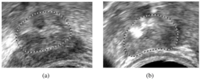
The prostate surrounds the urethra from the base, below the bladder, to the apex (Fig. 1). The urination is controlled with two sphincters located at the extremities of the prostatic urethra. As required for the intervention, a urinary probe is inserted in this canal. Thus, an acoustic shadow appears on each transverse slice, resulting in the lost of the upper edge. Another well known problem is the weakness of the edges at the apex and at the base (Fig. 2). In fact, the ultrasound beam is tangential to these boundaries and is not well reflected. Moreover, the bladder and the seminal vesicles look similar in appearance to the prostate. Therefore, the base is even more difficult to delineate.
Fig. 1. Ultrasound images of a prostate and its surrounding organs. The prostate appears darker and is not centered. Its boundary is almost well defined in this favorable case (central slices). Left: axial slice of the volume (the transducer being located on the lower, black area of the image). Right: sagittal slice.
Fig. 2. Axial ultrasound images of (a) the prostate base, (b) the prostate apex. The dashed contours represent the expert delineations. These pictures point out some of the segmentation problems. (a) Darker area represents the seminal vesi-cles. (b) White zones are mainly due to calcifications.
Fig. 3. Initialization: (a) ultrasound image with eight user-selected initial points; (b) initial mesh superimposed on the expert-defined surface.
III. METHODS
A. Initialization
The two algorithms presented in sections B and C are ini-tialized in a same way. This step is performed by positioning eight points , called initial points, on the boundary of the prostate [six in a central plane, one at the apex and one at the base, Fig. 3(a)]. Six of them are used to de-duce the center and the semi-axis of an ellipsoid which is then meshed. Next, a thin plate spline transform is applied so that the resulting mesh passes exactly through the initial points and better matches the prostate shape (see [22] for more details).
Because of the transrectal acquisition, the prostate is often close to the rectal wall. However, this wall has sometimes a higher contrast than the prostate and may lead to a failure of the segmentation algorithm. To avoid this, the mesh vertices
Fig. 4. Relocation of the mesh obtained from the eight initial points in the rectal wall area. (a) Rays, that cover an angle of about 120 , are thrown from the probe center and their intersection with the balloon boundary is searched (bright voxels).d is defined, along the ray that connects the probe center to the initial pointppp , as the distance between the balloon boundary andppp . (b) Another axial slice. Mesh vertices that are in the balloon or at a distance less thanminfd 0 2; 30g from the balloon boundary are relocated at a distance of d 0 2 from this boundary along the rays that connect them to the center probe, towards the prostate.
positioned in this area were relocated. This process aims at shifting the mesh closer to the prostate edge than to the rectal wall (without looking for an accurate positioning). The first step illustrated on Fig. 4(a) consists, for each axial slice, in tracing rays from the probe center to the balloon boundary, corre-sponding to the first bright voxels as the balloon is hypoechoic. The distance between the initial point and the balloon boundary, measured along the ray joining the probe center and is used as a reference. Next, the mesh vertices located in the balloon or at a distance less than from the balloon boundary are relocated at a distance of from this boundary along the rays that connect them to the probe center, towards the prostate [Fig. 4(b)]. The values of and 30 were deduced through experiments on a subset of the 3-D images and validated on the 3-D remaining images. Although the rectal wall thicknesses are highly variable between patients (see Figs. 1 and 2), good results were obtained in all cases. An example of the 3-D resulting mesh is given in Fig. 3(b).
B. Discrete Dynamic Contour
Once the initial mesh is built, the algorithm of discrete dy-namic contour [13] consists in applying at each vertex a total force which aims at deforming the surface. Using the dy-namic equations derived from Newton’s second law, the accel-eration deduced from the sum of forces at vertex enables to calculate its velocity and its new position from the pre-vious time step
(1) (2) (3) where is the mass at vertex and the time step. This process is iterated until all vertices stop moving or, more pre-cisely, until the acceleration and velocity of each vertex become
close to zero
(4) with a small positive constant. A large number of iterations may be necessary to reach equilibrium but the last iterations do not change significantly the final result. Thus, a maximum number of iterations is often fixed to stop the process even if convergence is not reached. Moreover, as the eight initial points were placed by an expert, they are considered as landmarks points and are not allowed to move.
corresponds to a weighted sum of external , in-ternal and damping forces:
(5) where the weights are equal for all vertices.
External forces drive vertices toward strong edges in their local neighborhood. is defined at voxel of coordinates as the gradient of an image potential energy function
(6) (7)
where “ ” is the gradient operator, is a Gaussian filter, “ ” is the convolution operator and is the image. Then, image force at vertex is given by
if
(8) where is the unit radial vector at vertex . is obtained by a trilinear interpolation from the image force field, corresponding to the real coordinates of vertex . Tangential components of forces are ignored in order to avoid vertices merging. Finally, as the prostate is most often darker than its environment, only forces derived from outward-pointing gradients, that is to say, directed along the normal, are kept fol-lowing the 2D implementation proposed by Ladak et al. [14].
Internal forces aim at smoothing the mesh during deforma-tion. The internal force proposed in [22] has the disadvantage of making the mesh shrunk in absence of image forces. There-fore, we used the expression reported in [21] that overcomes this drawback by minimizing the difference of mean curvature be-tween each vertex and its neighbors
(9)
where is the mean curvature of vertex estimated, in our study, by fitting a simple quadric , the coordinate being oriented along the normal . Like external forces, internal forces are oriented along the normals.
Damping forces ensure stability of dynamic behavior and pre-vent oscillations during deformation. They are proportional to the velocity
(10) with , a small negative constant.
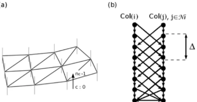
Fig. 5. Graph structure. (a) Vertical lines in blue at each vertex represent the set of voxels corresponding to a column of nodes in the graph. (b) Intra- and inter-column directed arcs.
C. Optimal Surface Detection
The method of Optimal Surface Detection [41] considers the segmentation problem in a volumetric image as the computation of the minimum s-t cuts in a weighted, oriented graph, with two auxiliary nodes and . The solution, that verifies smoothness constraints, corresponds to the surface with the minimum cost among all feasible surfaces in the volume and is thus optimal. Besides, this surface is found in a polynomial time (i.e., with respect to the number of nodes and arcs).
The algorithm relies on a mesh which represents an approx-imate segmentation of the sought object. In the present study, the mesh described at Section III-A was employed. This mesh is used to structure the graph and to define neighborhood rela-tionship between its nodes. Let us consider, for each vertex of the mesh, a set of voxels intersected by a ray oriented along the normal and distributed on both sides of the surface [Fig. 5(a)]. Each set is incorporated into the graph as a column of nodes . These nodes are then linked by two kinds of directed arcs of infinite weights. Intra-column arcs connect nodes of a same column from to
if . Inter-column arcs connect nodes of adjacent columns (11) where is the neighborhood of and is a smoothness con-straint [Fig. 5(b)]. For two adjacent nodes and
on the sought surface, the difference , can not be larger than .
In a second stage, a cost function based on image features is defined to assign to each node a cost value . becomes smaller as the voxel is more likely to belong to the targeted surface. A weight is then computed from the cost function such as
if ,
(12) The final stage consists in inserting a starting node (the source) and a terminal node (the sink) into the graph. Addi-tional directed arcs are created from the source to nodes with and from nodes with to the sink. In both cases, arcs capacities are equal to . Finally, the optimal surface that intersects one node of each column and minimizes globally the cost function is computed with an s-t cut algorithm [43].
From the experiments we have conducted, a few modifica-tions were brought allowing to improve slightly the method. Firstly, when applying the OSD to isotropic images, the depths of segments along which voxels are intersected spread from 20 inside to 30 voxels outside. In case of anisotropic images, the depth at vertex was adjusted by multiplying it by
(13)
where and is the spacing factor used to inter-polate the volume image along in order to get an isotropic volume.
Secondly, the cost function used to segment the prostate in ultrasound images was defined by
(14) with
(15) This function is inversely proportional to the gradient of the image smoothed by a Gaussian filter. The term was added to penalize gradients which are not oriented along the corre-sponding normal giving thus more weight to edges with dark to light grayscale transitions from inside to outside. In the case where the vertex is an initial point, particular cost values were given to nodes of
if
(16) in order to ensure that initial points belong to the sought optimal surface.
Thirdly, as the mesh is not isotropic, was modulated ac-cording to the distance between vertices
(17) where is the position of vertex , is a constant and is the integer part function. The value of controls the smoothness of the surface. But, even with an appropriate choice of this value, the resulting mesh may need an additional smoothing process to correct some unwanted irregularities. Thus, in a last stage, a fast regularization process was applied which consists in shifting vertices so that
(18) with the mean curvature of vertex of the initial mesh. In Section IV, OSD and OSDr correspond respectively to the OSD algorithm without and with the regularization process.
IV. PERFORMANCESTUDY
A. Protocol
The algorithms of DDC and OSD were evaluated separately or combined by applying the DDC on the output of OSD with regularization step. The experiments were performed on both anisotropic and isotropic 3-D images. As the prostate represents
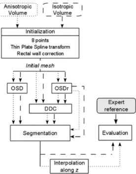
Fig. 6. Summary of the algorithms. DDC, OSD, OSDr: Optimal Surface De-tection followed by a regularization process. Dotted lines: anisotropic volume. Dashed lines: isotropic volumes.
a part of the volume, only a region of interest was taken into account. A bounding box was therefore defined as
(19)
where correspond to the coordinates of the initial points and , , and to the dimensions of the image along the , , and directions. The value of 75 was chosen to ensure that the prostate was always included in the region of interest. For anisotropic images, distances and cur-vatures were weighted to correspond to those of the isotropic images and the results were interpolated at the end to measure the true differences. The different approaches are summarized Fig. 6. As initial points at the base and the apex correspond to the extremities beyond which tissues must not be directly heated, the vertices beyond these limits were projected on the transverse plane containing the closer initial point or at the end of the process.
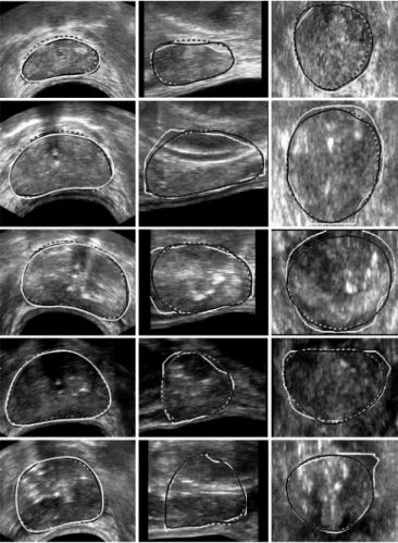
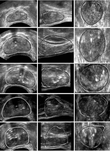
The performance of these algorithms was evaluated using 28 prostate volumes. These images were classified into three cat-egories according to the quality assessed by the expert: good, medium or poor quality, each group containing respectively 11, 11 and 6 samples. Omitting the base and the apex which are only exceptionally well-defined, good images exhibit sharp edges in the whole central part (Fig. 7, rows 1 and 2) whereas medium quality images display blurred boundaries in some areas (Fig. 7, rows 3 and 4). In poor quality images, prostate contours are on the overall badly-defined and the inside part of the gland is much more heterogeneous (Fig. 7, row 5).
Fig. 7. DDC segmentations (black with gray edge) compared with manual de-lineations (white). Dashed contours correspond to the initialization. Columns: axial, sagittal, and coronal sections of five isotropic 3-D images. Rows: from 1 to 5, two good, two medium, and one low quality images.
For each volume image, three initial meshes were defined. As the shapes of the meshes depend on the manually-selected point locations, different central planes and various apex and base positions were used.
The resulting segmented surfaces were compared to manu-ally outlined prostates. The 28 volumes were analyzed and man-ually delineated by two physicians. Ten volume images were contoured twice by the same physician, with a few months in-terval in between to get a rough estimation of the intra-observer variability.
B. Metrics
The evaluation of the segmentation results was performed by computing volume-based and distance-based metrics. Sensi-bility (Se) and volume overlap (VO) were employed as volume-based metrics
(20) (21)
where and are manually and semi-automatically seg-mented volumes.
To compute distance-based metrics, the distance from a point to a surface was defined as
(22)
The symmetric average surface distance between the manually obtained surface and the semi-automatically generated one
was then calculated by
(23)
with , the number of voxels belonging to . Furthermore, maximum deviations were measured using Hausdorff distances
(24)
C. Results
The performance of the two algorithms, i.e., DDC and OSD, has been evaluated qualitatively by visual comparison with the expert-defined contours in a first step, and then, quantitatively conducted using the metrics described above. Both steps are sig-nificant because global indexes may hide some local discrepan-cies of clinical relevance.
The parameters of the DDC were set to ,
for simplicity (1)–(3), (4), , , (5), (10), the variance of the Gaussian filter and the maximum number of iterations was set to 200 as the deformations that occur beyond this value are negligible. , and were adjusted by varying their values over a large variation interval. The quality of the resulting segmentations was measured on a training subset of 14 randomly selected spec-imens among the 28 in order to deduce the best parameter set. These latter were then tested on the remaining 14 specimens. The process was iterated 100 times to change the training subset. As the choice of is less sensitive [14], it was not optimized. For OSD, the conducted experiments, identical to those applied for the DDC, have shown that offered the best com-promise between a value sufficiently high to allow sharp local variations that may occur in prostate shapes and sufficiently low to limit irregularities.
Some examples of the resulting segmentations, obtained on isotropic volumes, are displayed Figs. 7 and 8, with axial - , sagittal - , and coronal - sections. A slice by slice inspection has been visually performed by one of the experts by projecting simultaneously the expert contour and the results obtained by the algorithms. The overall comparison with the manual delineations pointed out that the OSDr method better follows the boundary of the prostate.
However, the DDC provides rather good results when the organ is well-contrasted but also on low quality images as it can be seen on the dataset 5. Indeed, this method works locally around the initial mesh and does not move far away from it.
Fig. 8. OSDr segmentations (black with gray edge) compared with manual de-lineations (white). Dashed contours correspond to the initialization. Columns: axial, sagittal and coronal sections of the same isotropic 3-D images as Fig. 7.
Thus, if the initialization is well-localized, the results are cor-rect. However, if the initial mesh is not close enough to the sought edges or if it is positioned on local minima, noticeable differences with the ground truth may appear.
The OSD algorithm integrates image features over a larger neighborhood around the initial mesh and provides a global op-timization leading to a better segmentation than the DDC. Er-rors occur nevertheless when the prostate shape varies sharply or when the initialization is too far from the boundary. Besides, the optimum does not always correspond to the prostate edge as illustrated on the coronal section of image 2 (Fig. 8). In this case, the apex is much less contrasted than its surrounding which dis-turbs the algorithm. On the other hand, we can observe than the DDC is less distant from the boundary in this zone.
The quantitative evaluation was carried out on isotropic and anisotropic volumes. The results are summarized Table I. These statistics are issued from the 28 specimens, each segmented using three different initial meshes and all expert references. It appears that the performance obtained by using the DDC is slightly inferior to the one provided by the OSD (about 3% in Se and VO, 0.2 mm at most for SASD). This difference is a little bit increased with the addition of the regularization process which corrects some parts of the optimal surface that are not well positioned by moving them away from strong but false edges. Smoothness constraints are only taken into account in
TABLE I
QUANTITATIVECOMPARISONSBETWEEN THESEGMENTEDSURFACES OBTAINEDWITH THEALGORITHMS AND THEMANUALLYOUTLINED PROSTATES. ALGORITHMSWEREAPPLIED ON28 3-D IMAGES. EACHSPECIMEN WASSEGMENTEDTHREETIMESFROMTHREEDIFFERENTINITIALMESHES.THE RESULTINGSEGMENTATIONSWERECOMPARED TOMANUALDELINEATIONS FROMONEEXPERT BYCOMPUTING THESE, VO, SASD,ANDHD. VALUES PRESENTED ARE THEMEANS AND THESTANDARDDEVIATIONS(AFTER THE6 SIGN)OF ALLTHESEMEASURES. FOR THESASD AND THEHD METRICS,THEVALUES AREGIVEN INMILLIMETERS AND,INPARENTHESIS,
INVOXELS
this case. Applying the DDC, for which the output of the OSDr provides a better initialization, drives the surface toward other boundaries and globally enlarges the segmentation as it is shown by the increase of the sensitivity. This combination of the OSDr with the DDC brings some improvement except for the Haus-dorff distances which are increased but this improvement does not seem really significant. Besides, we can observe that the al-gorithms are somewhat more efficient when applied on isotropic images but, here too, the benefits remain low.
Table II provides a comparison between the intra-observer variability and the segmentation results. It can be seen that they have very close values. However, the variances observed be-tween the two manual delineations for the low quality image samples are much higher than the ones obtained by the semi-au-tomatic algorithms.
Table III describes the same statistics using as reference the deviations between the two expert manual delineations and for the all 28 specimens. It shows that the three algorithms lead to error values in the same range and an overall good performance in particular for SASD and HD with a slightly better behavior of OSDr. The variances between experts are, here also, higher than those produced by the algorithms for poor quality images.
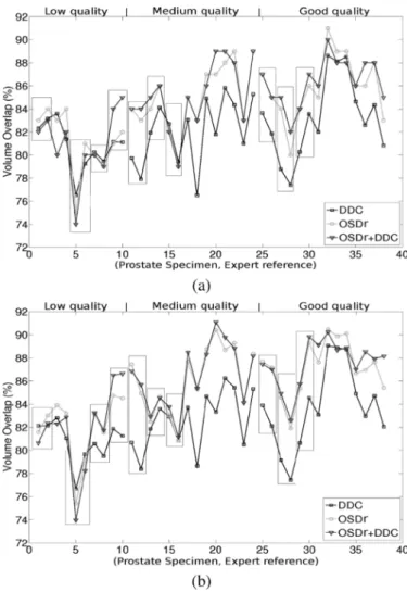
Fig. 9 illustrates volume overlap values produced by the dif-ferent algorithms for each specimen. Each point corresponds to the mean of the volume overlap measures obtained by com-paring the three segmentations produced from the different ini-tial meshes to one expert delineation. Black rectangles represent 3-D images for which two expert references from one physi-cian are available. The performance of the algorithms either on anisotropic images [Fig. 9(a)] or on isotropic images [Fig. 9(b)] remains relatively equivalent with a little gain for some isotropic datasets. Results for low, medium and good quality images are
TABLE II
COMPARISONBETWEEN THEFIRSTExp AND THESECONDExp SETS OF CONTOURSDRAWN BYEXPERT1. THESEDELINEATIONSWEREOBTAINED ON 10 VOLUMESWHOSETHREE ARE OFGOODQUALITY(G), THREE OFMEDIUM QUALITY(M),ANDFOUR OFPOORQUALITY(P). VALUESPRESENTED ARE THEMEANS AND THESTANDARDDEVIATIONS(AFTER THE6 SIGN)OF THE
METRICS(SE, VO, SASD,ANDHD) WHERE THELASTTWO AREGIVEN INMILLIMETERSAND,INPARENTHESIS,INVOXELS). THECOMPARISON WASALSODONEBETWEEN THESEMI-AUTOMATICSEGMENTATIONS OF THE
ANISOTROPICVOLUMESANDExp ON THESAMESET OFIMAGES
TABLE III
COMPARISONBETWEEN THEFIRST SET OFCONTOURSFROMEXPERT1 Exp AND THE SET OFCONTOURFROMEXPERT2 Exp . THESEDELINEATIONS WEREOBTAINED ON28 3-D IMAGESWHOSE11ARE OFGOODQUALITY (G), 11ARE OFMEDIUMQUALITY(M),ANDSIX ARE OFPOORQUALITY(P). THEVALUESPRESENTED ARE THEMEANS AND THESTANDARDDEVIATIONS (AFTER THE6 SIGN)OF THEMETRICS(SE, VO, SASD,ANDHD) WHERE THE
LASTTWO AREGIVEN INMILLIMETERSAND,INPARENTHESIS,INVOXELS) MEASURED ONTHESEIMAGES OFDIFFERENTQUALITIES. THECOMPARISON WASALSODONEBETWEEN THESEMI-AUTOMATICSEGMENTATION OF THE
ANISOTROPICVOLUMES ANDExp ON THESAME SET OFIMAGES
represented from left to right. A trend can be observed when going from low to good quality images. The behavior of the
Fig. 9. Volume overlap obtained separately for each prostate specimen in the case of anisotropic (a) and isotropic (b) volumes. Each point corresponds to the mean of the volume overlap measures obtained by comparing the three seg-mentations produced from the different initial meshes to one expert delineation. Black rectangles represent 3-D images for which two references from the same expert are available.
DDC is quite similar to the other algorithms for low quality im-ages. For medium and good categories, the OSD-based methods provide better results. The comparison of the segmentations pro-vided by the OSDr alone or combined with the DDC shows that they are often equivalent even if in some cases differences can be noticed.
A regional study has been carried out in order to go further in our analysis. As the edges at the base and the apex are clearly less defined than in the central part, this study aimed at eval-uating the errors independently in each of these areas. Consid-ering the set of axial slices contained in the expert reference, the first and last 20% were assigned to the extremities, and the re-maining 60% to the central region. Thus, the total slice thickness comprising the extremities ranges from 6 to 10 mm, distances that are equal or slightly higher than the margins took during the treatment to preserve the sphincters located in these zones.
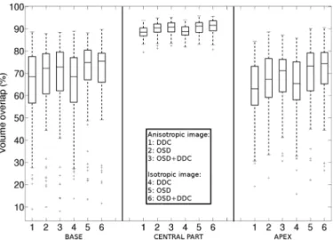
Fig. 10 highlights that errors are notably reduced in the cen-tral part when compared with the base and the apex ones. In-deed, the volume overlap is close to 90% with a small disper-sion for all the algorithms. Results provided by the DDC are similar whether the 3-D images are isotropic or not while the
Fig. 10. Regional evaluation of the volume overlap produced by the algorithms separately for the base, the central part, and the apex.
OSD-based methods display a higher dispersion when applied on anisotropic images at the base. Moreover, at this extremity, coupling DDC with OSDr does not bring an added-value. At the apex, the combination of OSDr and DDC increases the median value and decreases the dispersion leading to a better segmen-tation in this region. Indeed, the apex zone presents less sur-rounding structures than the base to mislead the algorithm.
To go a step further in the objectivation of the results, a statistical study was performed. Each method (DDC, OSD, OSDr, and was applied on the 28 3-D images and four metrics were measured by comparison of the results with the ground truth. Each couple (3-D image, method) was thus described with four values: the average distances (SASD), the standard deviations of these distances , the Haus-dorff distance (HD) and the mean of the 10% of the maximum distances . Given that three initial meshes were used per volume, these metric values correspond to an average of the measures obtained by comparison of the three resulting seg-mentations with the expert reference. The comparison between methods was done using repeated measures mixed ANOVA models [44]–[46] where the observed volume was considered as a random effect and the other factors (methods and metrics) as fixed effects.
1) Study 1: First, we compared the four methods for
each metric separately, using the following two-factor mixed ANOVA model
(25) with to 28 (volumes) and to 4 (methods). is the value observed for the th volume, assessed by the method , is the global level observed across all the volumes and the methods, is the random effect of the volume (random vari-able: ), is the global level observed for the method (fixed effect), and is the residual value observed for the volume assessed by method after taking into account the global level of volume and method . Post-hoc compar-isons between methods were done using t-tests, with a correc-tion for multiple comparisons (Tuckey method). P-values, that correspond to the estimated probabilities of rejecting the null
hypothesis that means are equal when the means are actually equal, were then deduced. Means were thus considered as statit-ically significantly different if the p-value was lower than the 5% level of significance.
2) Study 2: To test the global effect of the four methods when
considering the four metrics simultaneously, we used a three-factor mixed ANOVA model, including the metric effect as a fixed effect
(26) with 1–28 (volumes), 1–4 (methods), 1–4 (met-rics). is the value observed for the th volume, assessed by the method and the metric , is the global level ob-served across all the volumes, metrics and methods, is the global level observed for the volume [random variable
], is the global level observed for the method (fixed effect), is an interaction term between method and metric (fixed effect) and is the residual value observed for the volume assessed by the method and the metric after taking into account the global level of volume , method and metric [random variable: ]. Again, post-hoc comparisons between methods were done as above.
These analyses were performed globally on the whole prostate, but also in a regional way (base, middle part, apex) to locate the differences. The segmentation results were compared to experts 1 and 2. SAS software (SAS 9.1, SAS Institute Inc., Cary, NC) was used to carry out this study.
The interpretation of these statistics led to the following con-clusions.
• The differences are statistically significant between the re-sults obtained with the DDC and the OSD methods, at the base and at the apex according to the studies 1 and 2. The adjusted p-values are less than 0.2% when all the met-rics are considered simultaneously or when the SASD, the and the metrics are analyzed individually. • The differences are statistically significant between the re-sults obtained with the OSD and the OSDr algorithms, globally and mainly in the central part of the prostate with adjusted p-values less than 0.01% with the study 2 and less than 0.1% with the study 1 for almost all the metrics and all the experts (1 exception ). The differences at the base and the apex are mainly significant between HD met-rics (adjusted p-values ).
• The differences are statistically significant between the re-sults obtained with DDC and OSDr methods, globally and for all the subvolumes (base, middle part and apex) with the studies 1 and 2. The adjusted p-values are less than 0.2% for the whole prostate, the base and the apex. In the central part, the adjusted p-values are less than 5% with the study 2. The study 1 shows that these differences occur between the SASD and the metrics . Finally, the differences between OSDr and do not appear statistically significant.
V. DISCUSSION
Several major issues must be emphasized concerning the re-sults described above. Our main objective was to find a 3-D
so-lution which satisfies the constraints imposed by the HIFU treat-ment as the accuracy (depending on the margins took during the intervention), the computational time and the user interaction. It was also to provide an evaluation with expert ground-truth on a significant number of datasets and a comparison with already reported solutions.
The explored solutions make use of the same initial con-ditions starting with only eight points on which a first ap-proximation of the global shape of the prostate is built. The
a priori information brought by the initial points, notably at
the base, at the apex and in the acoustic shadow produced by the urinary probe allows to constrain the segmentation which would otherwise tend to “leak.” The influence of the positioning of these landmarks has been incorporated in our study. The automatic relocation of the part of the mesh close to the rectal wall (depicting sometimes different shells) avoids the algorithms being attracted by high local gradients. Moreover, this initialization is well adapted to the HIFU therapy. Indeed, when starting the therapy, the physician defines the location of the base and of the apex to ensure that the treatment is not applied beyond these limits. Locking the initial points during the segmentation process preserves these margins.
On the overall, the performance achieved by the algorithms is rather high when visually examined by experts and quantita-tively assessed by using different metrics. The differences ob-served are in the same range that the intra- and inter-observer variabilities. They make appear that the errors measured for the whole prostate and including poor quality images are in all cases around 90% for the sensitivity. The most efficient solutions lead to a volume overlap of about 85% and a symmetric average sur-face distance less than 1 mm. The Hausdorff distance however shows that deviations can go up to 5 mm but still remain com-parable to the intra- and inter-observer range. These expert ref-erences suffer of the fact that they are performed slice to slice, with a risk to loose the 3-D continuity even if the interactive tools allow them to navigate into the whole volume whereas the 3-D algorithms ensure this continuity.
The cost function (14) was adapted from [47] to ultrasound images of prostate. While Heimann et al. [40] combined the OSD with a statistical shape model and an appearance model also based on gradient features, the resulting statistical figures are equivalent to those of our approaches. It must be noticed that errors occur, in both cases, essentially at the extremities which is common to most of the methods reported in the literature.
The results, assessed both qualitatively and quantitatively, produced by the DDC algorithm are often on the overall inferior to those provided by the OSD and OSDr owing in particular to a higher sensitivity to the initialization. This was confirmed by the statistical study based on mixed ANOVA models that showed that significant differences can, in particular, be noticed at the base and at the apex which are critical areas. But the choice of parameter values also affects the final segmentation. Indeed, the parameters and were adjusted following the system-atic and random procedure described in the results section but slight local deviations from the true contours can still be ob-served. A potential perspective for DDC may consist in modu-lating the weights of the internal and external forces according to the local noise level or to prior anatomical knowledge. This is
not a trivial problem because the noise is non-stationary and the prostate shapes and sizes are rather patient-dependent. In OSD, reducing the value of when the shape of the prostate is more regular could limit errors. But the regularization stage applied on the output of OSD corrects most of these errors and allows choosing a value of adapted to most prostate shapes (following the procedure mentioned just above for DDC). Therefore, the OSDr algorithm is less sensitive to the choice of the parameter values than the DDC.
Additional attempts not reported here have been carried out by looking for candidate points with high gradients within the neighborhood of each mesh vertex but they did not bring signif-icant improvements. Texture was also examined in and out the prostate [48] with the idea to incorporate this information into DDC. However, if it has some relevance on well contrasted re-gions (i.e., the central part of the prostate), texture features do not bring new cues around the base and the apex, the most sen-sitive areas as it has been shown through the regional analysis we have worked out.
The methods used to segment the prostate, as pointed out in the introduction, must be fast considering the intra-operative con-straints. On anisotropic images, the detection of the rectal wall and the Gaussian filtering, which are common stages to DDC and OSD, take about 0.2 s and 10 s respectively on a 2.33 GHz Xeon PC. The computation time of the remaining steps for the DDC is around 8 s whereas the OSD algorithm requires less than one second. The latter is thus faster and therefore more compat-ible with the treatment constraints. For the isotropic images, the computation time is multiplied by a factor almost equal to 2.6. Given that the improvement brought by applying the algorithms on isotropic images is limited and that the prostate segmentation must be repeated during the operation, the best compromise con-sists in working on the original, anisotropic volumes.
To summarize, the experts made the following comments on the above results. When compared to intra- and inter-observer variabilities, and according to the margin constraints imposed by the treatment at the extremities (apex and base), these re-sults enable to consider the definition of the protocol of the high intensity shot distribution in a quasi-automatic way. The rectal wall and the prostate area in its immediate surroundings are particularly critical: the former, in order to avoid any poten-tial damage, the latter, because most of the tumors are located in this region. Moreover, this segmentation, replacing a manual delineation that could take about 15–25 min depending on the qualities and the sizes of the specimens, saves a significant time for the intra-operative application.
The HIFU therapy is a fast evolving technique and many improvements can be expected either on the imaging side or in more focussed treatments. MRI information will very likely play an important role in the future, not only by its capability to monitor the temperature changes but also by the possibility to get a better definition of the prostate boundaries in particular at the apex and the base. Preoperative MRI acquisitions also open new paths for segmenting intra-operative ultrasound images by matching the two modalities. In addition, MR images may allow depicting the tumoral regions inside the prostate, thus, offering a way to treat well targeted areas instead to destroy the whole organ.
VI. CONCLUSION
Two main frames, based on discrete dynamic contour and op-timal surface detection, with several variants, have been pro-posed in this paper for a semi-automatic segmentation of the prostate in high intensity ultrasound protocols. They have been evaluated on a rather large dataset using identical initial condi-tions. This evaluation has been conducted on the whole prostate volume and on different subsections of the prostate. The re-sulting segmentations have been compared through different metrics with manually expert delineations. Differences were an-alyzed with statistical models to determine their significativity. In all cases, operating in 3-D with a limited interactivity re-quested to the user appears as an important advantage.
All these methods have some merits and have shown on the overall a quite good performance, either on anisotropic (data without any preprocessing) or isotropic (after interpolation) volumes. They always fall within the intra- and inter-observer variability interval. However, the OSD-based approach pro-vides slightly better results in terms of accuracy and requires less computation resources, a major constraint for the clinical application. Some deviations from expert-defined contours may still be observed at the apex and the base, where boundaries are missing but fulfill the constraints (i.e., the margins defined by the physician to protect the sensitive surrounding structures) imposed by the therapeutic protocol. In addition to the inte-gration of these algorithms in HIFU platforms with optional correction tools, the work currently in progress concerns the application of these methods to MR an CT images of the prostate.
ACKNOWLEDGMENT
The authors would like to thank E. Blanc, L. Brasset, V. Rocher, D. Velut, and C. Vurpillot from EDAP-TMS for the help they provide in accessing the datasets and for the data acquisitions on the Ablatherm platform.
REFERENCES
[1] Cancer facts and figures Am. Cancer Soc., 2010 [Online]. Available: http://www.cancer.org
[2] European Cancer Observatory [Online]. Available: http://eu-cancer. iarc.fr
[3] C. A. Damianou, K. Hynynen, and X. Fan, “Evaluation of accuracy of a theoretical model for predicting the necrosed tissue volume during focused ultrasound surgery,” IEEE Trans. Ultrason. Ferroelectr. Freq.
Control., vol. 42, no. 2, pp. 182–187, Mar. 1995.
[4] L. Curiel, F. Chavrier, B. Gignoux, S. Pichardo, S. Chesnais, and J. Y. Chapelon, “Experimental evaluation of lesion prediction modelling in the presence of cavitation bubbles: Intended for high-intensity focused ultrasound prostate treatment,” Med. Biol. Eng. Comput., vol. 42, no. 1, pp. 44–54, Jan. 2004.
[5] R. G. Aarnink, R. J. Giesen, A. L. Huynen, J. J. de la Rosette, F. M. Debruyne, and H. Wijkstra, “A practical clinical method for contour determination in ultrasonographic prostate images,” Ultrasound Med.
Biol., vol. 20, no. 8, pp. 705–717, 1994.
[6] R. G. Aarnink, S. D. Pathak, J. J. de la Rosette, F. M. Debruyne, Y. Kim, and H. Wijkstra, “Edge detection in prostatic ultrasound images using integrated edge maps,” Ultrasonics, vol. 36, no. 1–5, pp. 635–642, Feb. 1998.
[7] Y. J. Liu, W. S. Ng, M. Y. Teo, and H. C. Lim, “Computerised prostate boundary estimation of ultrasound images using radial bas-relief method,” Med. Biol. Eng. Comput., vol. 35, no. 5, pp. 445–454, Sep. 1997.
[8] C. K. Kwoh, M. Y. Teo, W. S. Ng, S. N. Tan, and L. M. Jones, “Out-lining the prostate boundary using the harmonics method,” Med. Biol.
Eng. Comput., vol. 36, no. 6, pp. 768–771, Nov. 1998.
[9] S. D. Pathak, V. Chalana, D. R. Haynor, and Y. Kim, “Edge-guided boundary delineation in prostate ultrasound images,” IEEE Trans. Med.
Imag., vol. 19, no. 12, pp. 1211–1219, Dec. 2000.
[10] W. D. Richard and C. G. Keen, “Automated texture-based segmenta-tion of ultrasound images of the prostate,” Comput. Med. Imag. Graph., vol. 20, no. 3, pp. 131–140, May 1996.
[11] P. Abolmaesumi and M. R. Sirouspour, “An interacting multiple model probabilistic data association filter for cavity boundary extrac-tion from ultrasound images,” IEEE Trans. Med. Imag., vol. 23, no. 6, pp. 772–784, Jun. 2004.
[12] S. S. Mahdavi, W. J. Morris, I. Spadinger, N. Chng, O. Goksel, and S. E. Salcudean, “3-D prostate segmentation in ultrasound images based on tapered and deformed ellipsoids,” in Proc. MICCAI, 2009, vol. 5762, pp. 960–967.
[13] S. Lobregt and M. A. Viergever, “A discrete dynamic contour model,”
IEEE Trans. Med. Imag., vol. 14, no. 1, pp. 12–24, Mar. 1995.
[14] H. M. Ladak, F. Mao, Y. Wang, D. B. Downey, D. A. Steinman, and A. Fenster, “Prostate boundary segmentation from 2D ultrasound images,”
Med. Phys., vol. 27, no. 8, pp. 1777–1788, Aug. 2000.
[15] B. Chiu, G. H. Freeman, M. M. A. Salama, and A. Fenster, “Prostate segmentation algorithm using dyadic wavelet transform and discrete dynamic contour,” Phys. Med. Biol., vol. 49, no. 21, pp. 4943–4960, Nov. 2004.
[16] N. D. Nanayakkara, J. Samarabandu, and A. Fenster, “Prostate seg-mentation by feature enhancement using domain knowledge and adap-tive region based operations,” Phys. Med. Biol., vol. 51, no. 7, pp. 1831–1848, Apr. 2006.
[17] Y. Wang, H. N. Cardinal, D. B. Downey, and A. Fenster, “Semiau-tomatic three-dimensional segmentation of the prostate using two-di-mensional ultrasound images,” Med. Phys., vol. 30, no. 5, pp. 887–897, May 2003.
[18] M. Ding, B. Chiu, I. Gyacskov, X. Yuan, M. Drangova, D. B. Downey, and A. Fenster, “Fast prostate segmentation in 3-D TRUS images based on continuity constraint using an autoregressive model,” Med. Phys., vol. 34, no. 11, pp. 4109–4125, Nov. 2007.
[19] K. Diaz and B. Castaneda, “Semi-automated segmentation of the prostate gland boundary in ultrasound images using a machine learning approach,” in Proc. SPIE Med. Imag., San Diego, CA, 2008, vol. 6914, pp. 69144A–69144A-8.
[20] L. Wei, R. Narayanan, D. Kumar, A. Fenster, A. Barqawi, P. Wera-hera, E. D. Crawford, and J. S. Suri, “Bidirectional segmentation of prostate capsule from ultrasound volumes: An improved strategy,” in Proc. SPIE, Med. Imag., San Diego, CA, 2008, vol. 6914, pp. 69143W–69143W-7.
[21] A. Ghanei, H. Soltanian-Zadeh, A. Ratkewicz, and F.-F. Yin, “A three-dimensional deformable model for segmentation of human prostate from ultrasound images,” Med. Phys., vol. 28, no. 10, pp. 2147–2153, Oct. 2001.
[22] N. Hu, D. B. Downey, A. Fenster, and H. M. Ladak, “Prostate boundary segmentation from 3-D ultrasound images,” Med. Phys., vol. 30, no. 7, pp. 1648–1659, Jul. 2003.
[23] Y. Yu, J. A. Molloy, and S. T. Acton, “Segmentation of the prostate from suprapubic ultrasound images,” Med. Phys., vol. 31, no. 12, pp. 3474–3484, Dec. 2004.
[24] B. Li and S. T. Acton, “Automatic active model initialization via poisson inverse gradient,” IEEE Trans. Imag. Process., vol. 17, no. 8, pp. 1406–1420, Aug. 2008.
[25] Y. Zhang, R. Sankar, and W. Qian, “Boundary delineation in transrectal ultrasound image for prostate cancer,” Comput. Biol. Med., vol. 37, no. 11, pp. 1591–1599, Nov. 2007.
[26] A. Zaim and J. Jankun, “An energy-based segmentation of prostate from ultrasound images using dot-pattern select cells,” in Proc. IEEE
ICASSP, Honolulu, HI, 2007, vol. 1, pp. 297–300.
[27] F. Shao, K. V. Ling, and W. S. Ng, “3-D prostate surface detection from ultrasound images based on level set method,” in Proc. MICCAI, 2002, vol. 2489, pp. 389–396.
[28] A. Barqawi, L. Lu, E. D. Crawford, and S. S. Jasjit, “Semi-automated versus automated prostate boundary estimation from 3-D transrectal ultrasound images,” Int. J. CARS, vol. 2, pp. 134–137, 2007. [29] A. C. Hodge, A. Fenster, D. B. Downey, and H. M. Ladak, “Prostate
boundary segmentation from ultrasound images using 2D active shape models: Optimisation and extension to 3-D,” Comput. Methods
Pro-grams Biomed., vol. 84, no. 2, pp. 99–113, Dec. 2006.
[30] N. Betrouni, M. Vermandel, D. Pasquier, S. Maouche, and J. Rousseau, “Segmentation of abdominal ultrasound images of the prostate using a priori information and an adapted noise filter,” Comput. Med. Imag.
[31] F. A. Cosío and B. L. Davies, “Automated prostate recognition: A key process for clinically effective robotic prostatectomy,” Med. Biol. Eng.
Comput., vol. 37, no. 2, pp. 236–243, Mar. 1999.
[32] F. A. Cosío, “Automatic initialization of an active shape model of the prostate,” Med. Image Anal., vol. 12, no. 4, pp. 469–483, Aug. 2008. [33] R. Y. Wu, K. V. Ling, and W. S. Ng, “Automatic prostate boundary
recognition in sonographic images using feature model and genetic al-gorithm,” J. Ultrasound Med., vol. 19, no. 11, pp. 771–782, Nov. 2000. [34] L. Gong, S. D. Pathak, D. R. Haynor, P. S. Cho, and Y. Kim, “Para-metric shape modeling using deformable superellipses for prostate seg-mentation,” IEEE Trans. Med. Imag., vol. 23, pp. 340–349, Mar. 2004. [35] L. Gong, L. Ng, S. D. Pathak, I. Tutar, P. S. Cho, D. R. Haynor, and Y. Kim, “Prostate ultrasound image segmentation using level set-based re-gion flow with shape guidance,” in Proc. SPIE, Med. Imag., San Diego, CA, 2005, vol. 5747, pp. 1648–1657.
[36] I. B. Tutar, S. D. Pathak, L. Gong, P. S. Cho, K. Wallner, and Y. Kim, “Semiautomatic 3-D prostate segmentation from TRUS images using spherical harmonics,” IEEE Trans. Med. Imag., vol. 25, no. 12, pp. 1645–1654, Dec. 2006.
[37] C. Knoll, M. Alcaniz, V. Grau, C. Monserrat, and M. C. Juan, “Out-lining of the prostate using snakes with shape restrictions based on the wavelet transform,” Pattern Recognit., vol. 32, no. 10, pp. 1767–1781, Oct. 1999.
[38] D. Shen, Y. Zhan, and C. Davatzikos, “Segmentation of prostate boundaries from ultrasound images using statistical shape model,”
IEEE Trans. Med. Imag., vol. 22, no. 4, pp. 539–551, Apr. 2003.
[39] Y. Zhan and D. Shen, “Deformable segmentation of 3-D ultrasound prostate images using statistical texture matching method,” IEEE
Trans. Med. Imag., vol. 25, no. 3, pp. 256–272, Mar. 2006.
[40] T. Heimann, M. Baumhauer, T. Simpfendörfer, H.-P. Meinzer, and I. Wolf, “Prostate segmentation from 3-D transrectal ultrasound using statistical shape models and various appearance models,” in Proc. SPIE, Med. Imag., San Diego, CA, 2008, vol. 6914, pp. 69141P–69141P-8.
[41] K. Li, X. Wu, D. Z. Chen, and M. Sonka, “Efficient optimal surface de-tection: Theory, implementation and experimental validation,” in Proc.
SPIE Med. Imag., San Diego, CA, 2004, vol. 5370, pp. 620–627.
[42] Q. Song, X. Wu, Y. Liu, M. Smith, J. Buatti, and M. Sonka, “Optimal graph search segmentation using arc-weighted graph for simultaneous surface detection of bladder and prostate,” in Proc. MICCAI, 2009, vol. 5762, pp. 27–835.
[43] Y. Boykov and V. Kolmogorov, “An experimental comparison of min-cut/max-flow algorithms for energy minimization in vision,” IEEE
Trans. Pattern Anal. Machine Intell., vol. 26, no. 9, pp. 1124–1137,
Sep. 2004.
[44] E. Demidenko, Mixed Models—Theory and Applications. New York: Wiley, 2004.
[45] R. Littell, G. Milliken, W. Stroup, R. Wolfinger, and O. Schabenberger,
SAS for Mixed Models. Cary, NC: SAS Inst., 2006.
[46] G. Verbeke and G. Molenbreghs, Linear Mixed Models for
Longitu-dinal Data. New York: Springer, 2009.
[47] M. Sonka, V. Hlavac, and R. Boyle, “Segmentation II,” in Image
Pro-cessing, Analysis and Machine Vision, 3rd ed. New York: Thomson Eng., 2007, ch. 7, sec. 7.7, pp. 306–319.
[48] K. Wu, C. Garnier, J.-L. Coatrieux, and H. Shu, “A preliminary study of moment-based texture analysis for medical images,” in Proc. IEEE