;;DOCUMI?
OFFoCEil.36
B
412
RESESACH
LBORbTOM F LECTROOICS
MASSACHUSETTS INSTITUTE OF TIZIO
DECISION-FEEDBACK EQUALIZATION
FOR DIGITAL COMMUNICATION OVER DISPERSIVE CHANNELS
M. E. AUSTIN
TECHNICAL REPORT 461
AUGUST 11, 1967
MASSACHUSETTS INSTITUTE OF TECHNOLOGY
RESEARCH LABORATORY OF ELECTRONICS
CAMBRIDGE, MASSACHUSETTS 02139
The Research Laboratory of Electronics is an interdepartmental laboratory in which faculty members and graduate students from
numerous academic departments conduct research.
The research reported in this document was made possible in part by support extended the Massachusetts Institute of Tech-nology, Research Laboratory of Electronics, by the JOINT SER-VICES ELECTRONICS PROGRAMS (U. S. Army, U. S. Navy, and U. S. Air Force) under Contract No. DA 28-043-AMC-02536(E); additional support was received from the U. S. Navy Purchasing Office under Contract N00140-67-C-0210.
Reproduction in whole or in part is permitted for any purpose of the United States Government.
MASSACHUSETTS
INSTITUTE OF TECHNOLOGY
RESEARCH LABORATORY OF ELECTRONICS
Technical Report 461
LINCOLN LABORATORY
Technical Report 437
August 11, 1967
DECISION-FEEDBACK EQUALIZATION
FOR DIGITAL COMMUNICATION OVER DISPERSIVE CHANNELS
M. E. Austin
This report is based on a thesis submitted to the Department of
Electrical Engineering at the Massachusetts Institute of
Tech-nology, May 12, 1967, in partial fulfillment of the requirements
for the Degree of Doctor of Science.
Abstract
In this report, a decision-theory approach to the problem of digital communication
over known dispersive channels is adopted to arrive at the structures of the optimal
and two sub-optimal receivers: the "conventional" and "decision-feedback"
equal-izers, both employing matched and transversal filters.
The conventional equalizer
is similar to some equalization modems finding current application, while the new
decision-feedback equalizer (as its name implies) utilizes its previous decisions in
making a decision on the present baud.
The parameters of these two equalizers are optimized under a criterion which
min-imizes the sum of the intersymbol interference and additive noise distortions appearing
at their outputs.
Algorithms for evaluating the performances of the conventional and
decision-feedback equalizers are developed, proving especially useful at high SNR
where simulation techniques become ineffective.
To determine the dependence of their performance and sidelobe-suppression
prop-erties upon SNR and transversal filter length, the new algorithms were used to study
the conventional and decision-feedback equalizers when they are applied in equalization
of the class of channels exhibiting the maximum realizable intersymbol interference.
In addition, error-propagation effects found to arise in the decision-feedback
equal-izer operation are studied.
High overall error rates (as found at low SNR) lead to a
threshold effect as the decision-feedback equalizer performance becomes poorer than
that of the conventional equalizer.
Despite such error-propagation behavior, however, the decision-feedback equalizer
is found to be considerably better than the conventional equalizer at all SNR and error
rates of practical importance, due to its sidelobe-suppression behavior; moreover,
its advantages become more pronounced, the higher the SNR and the greater the
chan-nel dispersion.
TABLE OF CONTENTS
I.
INTRODUCTION -
INTERSYMBOL INTERFERENCE
AND EQUALIZATION
1
II.
OPTIMAL AND SUB-OPTIMAL EQUALIZATION
7
A. Optimal Equalizer Structure
7
B.
Sub-Optimal Equalization - The Conventional Equalizer
12
III.
EQUALIZATION USING DECISION FEEDBACK
23
IV.
PERFORMANCE OF THE CONVENTIONAL EQUALIZER
31
A.
Maximal Distortion Channels
31
B.
Error Tree Algorithm
38
C. Conventional Equalizer Performance
43
V.
PERFORMANCE OF THE DECISION-FEEDBACK
EQUALIZER
51
A. Algorithm for Obtaining High SNR Performance
52
B.
Decision-Feedback Equalizer Performance
59
C.
Bounding Mean Recovery Time
72
VI.
CONCLUSIONS - SUGGESTIONS FOR FURTHER RESEARCH
79
Acknowledgments
84
References
85
iii
DECISION- FEEDBACK EQUALIZATION
FOR DIGITAL COMMUNICATION OVER DISPERSIVE CHANNELS
I. INTRODUCTION - INTERSYMBOL INTERFERENCE AND EQUALIZATION
Commercial and military demands for higher data rates in the transmission of digital information over dispersive media, such as telephone links and the HF ionospheric channel, are continually increasing. This has led to a widespread interest in the development of receivers capable of mitigating the familiar intersymbol interference effects which inevitably accompany such increased data rates. Receiver filters designed to partially compensate for the dispersive characteristics of channels, or for the intersymbol interference distortion occurring when pass-ing signals through dispersive channels, are referred to as" equalization" filters, or" equalizers."
The two principal objectives of this report are (a) to present a receiver structure which uses its previous decisions to reduce intersymbol interference in high-speed data transmission over dispersive channels - the decision-feedback equalizer, and (b) to compare the performance of this new equalizer structure with that of the conventional equalizer structure currently being
employed.
In Sec. II, we first derive the optimal receiver for the problem of interest: synchronous transmission of binary data over fixed, known dispersive channels. The main innovation here is in the approach to receiver design in the presence of intersymbol interference - equalization is attacked not as a problem in linear filtering theory as it has been previously, but rather from a decision-theory viewpoint. This leads to the equations which specify the operations the
re-ceiver must perform on its input to minimize its probability of error. Our interpretation of these equations results in the optimal equalizer structure, a nonlinear receiver which unfortu-nately is too complex and impractical to construct, but which is nonetheless of interest for the insight it affords us in considering sub-optimal equalization. By modifying the assumptions used in arriving at the optimal equalizer, we next derive a sub-optimal equalizer structure which we refer to as the "conventional" equalizer. We then determine the equations specifying those parameter settings of the conventional equalizer which minimize the distortion energy appearing at its output, and we prove the existence and uniqueness of their solution. Section II concludes with a discussion relating this present work to that of earlier authors.
Adding to the assumptions used in deriving the conventional equalizer structure, we further assume in Sec. III that the receiver has made no decision errors on previous bauds, leading to our derivation of the decision-feedback equalizer. After interpreting the operation of this new equalizer structure and the nature of its decision feedback, we optimize its parameters under a minimum total output distortion energy criterion. Next, we consider conventional and decision-feedback equalization with regard to the degrees of freedom associated with their respective structures, and their manner of treating the intersymbol interference arising from both past and future bauds. We conclude Sec. III with heuristic arguments for the error-propagation ef-fects anticipated in the operation of the decision-feedback equalizer.
With a view to obtaining a quantitative comparison of the performances of the conventional and decisionfeedback equalizers, in Sec. IV we begin by deriving the channels we wish to study -the maximal distortion channels. For channels with a given overall channel dispersion length, the maximal distortion channels exhibit the largest possible distortion under a sum of the side-lobe magnitudes distortion measure. We then seek a method of evaluating the performance of the conventional equalizer. After noting that a direct calculation of the performance is concep-tually possible but computationally impractical, we develop an alternative approach. A new
computational algorithm is derived for obtaining upper and lower bounds on the performance of the conventional equalizer to any specified degree of accuracy. The implementation of this al-gorithm is explained, and its efficiency is studied through its application to examples of interest. Next, we present the exact performance data on the conventional equalizer when it is applied to equalization of the maximal distortion channels, as determined using this new algorithm. Sec-tion IV concludes with a discussion of the effects of equalizer length on the performance, and of the trade-off possible between signal-to-noise ratio (SNR) and equalizer length at different levels of performance.
In Sec. V, we are concerned with determining the performance characteristics of the decision-feedback equalizer. Next to its overall error rates as a function of SNR for various channels, error-propagation effects are of prime concern. Because of the nonlinear nature of the decision-feedback equalizer structure, its performance was studied through digital simulations at low and intermediate SNR. However, at high SNR, errors occur too infrequently to determine the error rates and error-propagation behavior accurately through simulations of reasonable duration. Thus, we determine the necessary modifications to our earlier algorithm to develop a second algorithm - a mixture of computation and simulation - which overcomes this difficulty, enabling us to obtain the desired error rates as well as burst and guard-space data, even at high SNR. We next present the results of our performance studies at all SNR, with discussions of overall error rates, burst and guard-space data, and the effects of equalizer length on these quantities. Finally, we conclude Sec. V with a development of an efficient method of bounding the mean burst duration, by modeling error propagation as a discrete Markov chain process, enabling us to treat equalizer recovery from the burst-error mode as a first-passage-time problem. This technique, which we find to be applicable at intermediate SNR due to the correlation properties of the distortion appearing at the output of the decision-feedback equalizer, provides us with a method of obtaining bounds on the mean recovery time without having to resort to simulations.
Section VI includes our conclusions, and suggestions for further research. After discuss-ing threshold effects noted in the operation of the decision-feedback equalizer at low SNR, and its obvious advantages over the conventional equalizer at high SNR, we then compare both equal-izer performances to upper bounds to obtain some feeling for the degree to which each is sub-optimal. Differences in the performances of the two equalizers are then interpreted, and ex-plained in terms of their respective methods of treating intersymbol interference in general, and in terms of their residual noise and intersymbol interference distortions, particularly at high SNR. Based upon our error-burst and guard-space studies, we note the additional im-provements possible in the decision-feedback equalizer operation which one might realize through application of burst-error detecting and correcting coding schemes. Finally, we discuss briefly some issues which may be of interest in further research, such as extensions of the present work to handle colored noise, correlated message sequences, multilevel signaling schemes,
2
different types of decision-feedback data, and the sensitivity properties of the conventional and decision-feedback equalizers with respect to channel measurement errors.
Having outlined the purpose and content of this report, we will devote the remainder of Sec. I to presenting some background material of interest. First, we introduce an important device for implementing equalizers which has been employed in all equalization systems of recent de-velopment - the transversal filter; next, we point out the difference between channel equaliza-tion and equalizaequaliza-tion of intersymbol interference, and the desirability of the latter; finally, we present a classification of equalizers and brief descriptions of three adaptive equalizers cur-rently under development. Two of these adaptive equalizers employ decision feedback, but both for a different purpose than the decision-feedback equalizer presented in this report.
Early efforts at channel equalization date back to 1928, when Zobel1 published an extensive work on distortion correction using lumped RLC filters. For some time, such filters adequately provided the amplitude compensation desired for telephone circuits, for the ear proved rather insensitive to the phase distortions they generally introduced. With the development of televi-sion, and with digital communication aiming at increased data rates, phase distortion became of greater concern, leading to the work with the transversal filter reported by Kallmann2 in 1940. The analog transversal filter may be realized using a tapped-delay-line (TDL) terminated in its characteristic impedance, with a high-input-impedance amplifier at each tap,output. With the amplifier gains suitably chosen for the desired equalization properties, the amplifier outputs are summed to obtain the transversal filter output, as indicated in Fig. 1(a). Often, the TDL
(b)
Fig. 1. Transversal filter. (a) Block diagram of filter; (b) representation in this report of both analog and digital realizations.
3
4
____ ·_ _ ___ 1ul
input is sampled, the delay lines are replaced by digital shift registers, and the weighting and summing operations are performed digitally. Throughout this report, whether considering an-alog or digital realizations, we will draw transversal filters as shown in Fig. 1(b). The tap gains of the transversal filter can be set to render amplitude compensation without phase distortion, phase compensation without amplitude distortion, or both amplitude and phase compensation. Such versatility, coupled with the increasing speed and availability of computers for calculating and adjusting its gains, has caused the digital transversal filter to become increasingly impor-tant in recent years, as illustrated in the adaptive equalization systems described further below.
One of the first adaptive receivers designed to equalize a dispersive channel was the RAKE
system described by Price and Green.3 This system transmits wide-band message waveforms
which are correlated against their delayed replicas at the receiver to enable measurement of the amplitude and phase characteristics of the individual paths of a multipath medium such as the HF ionospheric channel. By use of these measurements to set the amplitude and phase of the tap gains of its transversal filter, the RAKE receiver achieves nearly optimum weighting of the waveforms received from each of the paths, and sums them coherently to form its output. Considering the low 45-bits/sec data rate it achieved on the HF ionospheric channel, the RAKE system represents a highly inefficient use of its 10-kHz bandwidth when compared, for example, with the less sophisticated Kineplex system which was designed for data rates of up to 3000bits/sec with a bandwidth of only about 3.4 kHz, and without attempting channel measurement. 5 This serves to illustrate that, for data transmission purposes, one should not necessarily strive to equalize the channel itself, but rather should consider equalization for a particular choice of signals to be transmitted over the channel, as pointed out in the following example.
It is easily shown through the z-transform approach to inverse filtering that, in the absence of significant noise, the discrete two-path channel of Fig. 2(a) can be equalized using the trans-versal filter of Fig. 1(b), if its taps are spaced by the time delay between the two paths T, and
1 13-42-10140J I"~~~~~ rT
(a)
O T(b)
bT I O T (C)Fig. 2. Example of channel vs equivalent channel equalization. (a) Channel impulse response, (b) signaling waveform to be em-ployed over channel, and (c) result of syn-t chronous sampling of channel output with
input waveform (b).
t
4
its gains are set according to the relationship an = (-b)n - i (see Ref. 6). If this equalizer is
truncated after N taps, there will be residual response having magnitude I blN On the other hand, suppose we plan instead to use the channel of Fig. 2(a) to transmit data using amplitude modulation of the signal waveform shown in Fig. 2(b), which has a baud duration T > . Syn-chronous sampling of the channel output as indicated in Fig. 2(c) renders a sampled waveform which may be equalized with a transversal filter with gains an = [-(bT/T)]n-1 and with tap spac-ing T. With this latter approach, it is seen that convergence of the tap gains is obtained more rapidly than before. Moreover, the tap spacings are independent of -, an important matter if
T is a time-varying quantity, for then the channel equalization receiver must employ many more
taps than are required by the intersymbol interference equalizer, which need only adjust its tap gains. This simple example points out that if one intends to transmit a signal s(t) over a dis-persive channel having an impulse response g(t), it is generally more efficient to minimize the intersymbol interference distortion appearing at the receiver output through equalization of the equivalent impulse response h(t) = s(t) ( g(t), rather than attempting to equalize the channel g(t) itself in order to be able to handle arbitrary s(t).
Equalization filters fall within three categories: fixed, automatic, and adaptive. Fixed equalizers are adjusted to provide the amplitude and phase compensation necessary to correct the average distortion characteristics of dispersive channels, while automatic and adaptive equalizers, on the other hand, have generally found application in synchronous data transmission to equalize the equivalent channel, i.e., reducing the intersymbol interference distortion at the sampling times. The automatic equalizers transmit their known pulse waveforms prior to data transmission, which they utilize in adjusting the tap gains of their transversal equalization
fil-ter (for example, see Ref. 7). Adaptive equalizers differ from the automatic equalizers in that they adjust their transversal filter parameters during data transmission, using either a sound-ing waveform or the message waveform itself to minimize the intersymbol interference distor-tion, thus indirectly obtaining equivalent channel measurement. Three such adaptive systems are described briefly below.
An adaptive equalizer named ADAPTICOM has been under study at Cardion Electronics, Inc. and has been reported by DiToro.8 This system uses approximately a 3-kHz bandwidth to achieve a degree of equalization by using a filter which is matched to the received waveform for a single pulse transmission, in cascade with a transversal filter. ADAPTICOM's parameter settings are determined by periodically interrupting the data transmission several times per correlation time of the channel and sounding the channel, although apparently no attempt is made to exploit
the correlation between the successive measurements to improve the accuracy of the resultant settings. The transversal filter centertap has unity gain, with the remaining tap gains set equal to their respective tap outputs, when a single received pulse is passed through the matched
fil-ter, at that instant when the centertap output attains its maximum value. Thus, ideally, the tap gains are set equal to the sampled autocorrelation function of the equivalent channel. DiToro states that such gains, together with proper adjustment of a single gain simultaneously affecting the total contribution of all but the centertap outputs, minimize the mean square distortion due to intersymbol interference at the output, although his mathematical basis for this has not yet been published. Performing satisfactorily in the laboratory using a multipath simulator, ADAPTICOM is being constructed for testing on an actual HF ionospheric link.
Lucky9 reports the development and testing of an adaptive equalizer using a digital trans-versal filter, for application to telephone-line equalization. Similar in other respects to
5
his earlier automatic equalizer (Ref. 10), Lucky' s adaptive equalizer uses decision feedback, enabling him to make iterative tap-gain adjustments to minimize the sum of the sidelobe mag-nitudes appearing at the output when the mainlobe is normalized to unity. This adaptive equal-izer enabled tracking of the slowly fluctuating telephone channel, of course, but it also rendered better tap-gain settings than Lucky's automatic equalizer because a much larger number of trans-mitted pulses were employed in arriving at the settings than was reasonable to permit in a pre-call sounding signal for the automatic equalizer. The equalization algorithm used by Lucky at-tempts to set as many of the sidelobes to zero as is possible within the constraint of a finite TDL length, while ignoring the additive noise which is reasonably low on telephone lines. Lucky shows that this works well for channels having an initial distortion less than unity. For channels with larger initial distortion, as eventually will occur with increasing the baud rate for any channel, the convergence of Lucky' s tap-gain-adjustment procedure may fail as he noted, and, in addition, large sidelobes can arise beyond the sidelobes zeroed by the transversal filter.
Another equalization system, ADEPT, is currently under development at Lincoln Laboratory, principally by Drouilhet and Niessen. This system uses a 63-tap TDL for equalization of tele-phone lines in the transmission of 8-level, 10,000-bits/sec data. ADEPT, which has an initial training period, continues to adjust its tap settings during data transmission. A pseudo-random sequence-is transmitted in addition to the message waveform and, through correlation against the same sequence at the receiver, ADEPT attempts to minimize the output distortion energy due to intersymbol interference. To minimize the degradation of the tap settings derived from correlation of the pseudo-random sequence with the message waveform, the message is sub-tracted out using decision feedback. Note that this represents a different, and apparently less efficient, application of decision feedback than that employed by Lucky (Ref. 9), in that the energy in the message waveform is being discarded rather than being utilized in achieving the tap-gain settings. The advantages to be obtained over Lucky' s adaptive equalizer, through use of a dif-ferent tap-adjustment procedure and increased filter length, will be determined in the near future when ADEPT will be tested over an actual telephone link.
6
II. OPTIMAL AND SUB-OPTIMAL EQUALIZATION
Here, we consider the problem of determining the structures of receivers for digital communication over a linear dispersive channel. As shown in the model of Fig. 3, during the kth -baud period of duration T, ks(t) is transmitted, where s(t) vanishes outside an interval of
t
width T and where ~k = +1 or -1, corresponding to hypotheses Hi and H0, respectively. Weassume that the equivalent channel impulse response, h(t) = s(t) ( g(t), is known to the receiver through prior measurement made either directly or indirectly, as in the case of the adaptive equalizers described in Sec.I. In addition, the channel has additive noise n(t) corrupting its out-put. Thus, the input to our receiver is
r(t) = Z kh (t - kT) + n(t) (1)
k
where here, and throughout the remainder of the report, Z denotes the summation for k = -o
to +0 unless otherwise noted. k
n( r(t) '- - s(t) g(t) + r(t) SIGNAL ACTUAL FILTER CHANNEL (k-1 (a) n(t) l. Xth(t) l + r(t) EQUIVALENT CHANNEL k-1 (b) 13-42-0141
Fig. 3. Dispersive channel communication model: (a) digital communication over noisy dispersive channel; (b) equivalent channel model, h(t) = s(t) ( g(t).
Given the received waveform Eq. (1) for all t, our problem is to obtain receivers for making decisions on the k.' We first derive the optimal receiver structure, and then a simpler sub-optimal receiver. We will refer to the latter receiver as the "conventional" equalizer, to dis-tinguish it from the "decision-feedback" equalizer to be presented in Sec. III.
A. OPTIMAL EQUALIZER STRUCTURE
In deriving the optimal receiver for the problem stated above, we make the following assumptions:
(1) The k are independent,
(2) H0 and Hi are equally likely, and
(3) n(t) is white Gaussian noise, of double-sided spectral height N0/2.
These assumptions are generally met in practice. The extension to colored Gaussian noise is straightforward, as discussed in Sec. VI. Under these assumptions, it is a well-known result
in statistical decision theory that, to make a decision on the zeroth baud as to the value of 0, the optimal receiver computes the likelihood ratio
p[r(t)l0 = +1]
p[r(t) |
0= -1]
If we define for convenience of notation the sets
- = {(klk < 0)
+ = {klk 0 >
then we may write
p[r(t) 0] = E E p[r(t)l
o-0,
(t] P[,
_+] +- (2) (3) (4) (5)where the summations are over all possible message sequences occurring before and after the zeroth baud, respectively. From Eq. (1) and Assumption (3), we may write
p[r(t)jI -, 0, +] = K exp -No
J
s
[r(t)- E k h(t-kT) dtlI-
kI
= K exp -s
r (t) dtl exp ,k r(t) h(t- kT) dt k x exp - E jkN
1 0 h(t-jT) j k = K1 exp[f Fkak-Z Z
j kbj-k] k j k h(t - kT) dtj (6)where we have defined K1 = K exp [-(1/NO) f r2(t) dt], and the quantities
a A 2k NS
bk N
r(t) h(t - kT) dt= r(t + kT) h(t) dt
h(t) h(t - kT) dt
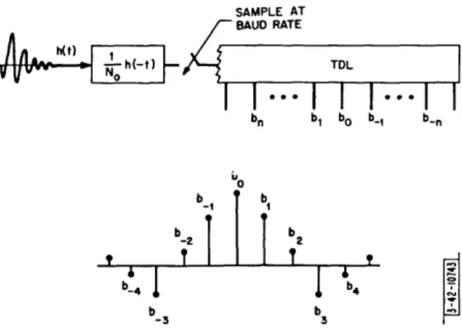
Note that all the information of the received waveform has been condensed into the set of suf-ficient statistics {ak), which may be generated as shown in Fig. 4. In Fig. 4(a), we see that the received waveform is input to a TDL, thus simultaneously making available the shifted versions of r(t) required in Eq. (7) where it is indicated that each tap output is to be multiplied by [(2/N0) x
h(t)] and the product integrated over all time t. Each integrator output will remain constant, however, after h(t) becomes zero (or negligibly small). Thus, if h(t) is nonzero only over the
8 and
(7)
2 No an a0 O-n (a) SAMPLE AT BAUD RATE h(-t) TDL MATCHED .. I FILTER an o 0 a n (b)
Fig. 4. Generation of sufficient statistics: (a) interpreting Eq. (7) directly, and (b) an alternative structure, a matched filter in cascade with a TDL.
interval (0, T1), then we may sample each integrator output at any time t > T to obtain the de-sired ak. Note that if we sample at t = T1, then we may replace the multiplication-integration operation on each tap output by a linear filter having an impulse response [(2/N0) h(-t)], since
the output of such filters will also render the desired ak at t = T1. Moreover, since the linear
filters common to each tap may be replaced by a single filter operating on the received waveform r(t) before it enters the TDL, and since the simultaneous sampling of each tap output may clearly be replaced by the sequential sampling of the waveform into the TDL at the baud rate 1/T, then an equivalent method of generating the sufficient statistics is as shown in Fig. 4(b). Thus, we note that optimal reception involves passing the received waveform through a filter matched
(except for the gain of 2/N0) to the equivalent channel impulse response h(t), sampling the matched
filter output at the baud rate to obtain the set of sufficient statistics {ak}, and then passing these into a TDL. Before considering the additional operations which the optimal receiver performs on these sufficient statistics, we first consider the bk sequence defined by Eq. (8).
From a comparison of Eqs. (7) and (8) and the discussion above, we observe that the bk se-quence may be generated using a structure identical (except for a gain of 2) to that of Fig. 4(b), if the input r(t) is replaced by h(t). But this corresponds to sampling the matched filter response to a single pulse transmission in the absence of noise, thus rendering (except for the gain of 1/No) the samples of the equivalent channel autocorrelation function, and bk = b k as indicated in
Fig. 5. Returning to Eqs. (5) and (6), we may write
p[r(t)il0 =
Z
Z
K2 exp[Z kak -Z Z
jkbj-k (9)- + k j k
where K2 = K1p(_, +) is a normalization constant, independent of _ and + through
Assump-tion (1). Factoring out the remaining terms which are independent of - and k+, we have
SAMPLE AT BAUD RATE bn 2
!
!
b-4 b-3 TDL T_~~~~~~~I I I -.- I
b1 bo b_! b-nI
b
4 b $Fig. 5. Generation of bk sequence of Eq. (8), the sampled autocorrelation function of the equivalent channel impulse response.
p[r(t)Io] = K
2 exp[ oao0-2
i2bo]
2
i 1
4
+
exp[
k#0 4 kakj k
j k¢=j
(j kbj-k]
(10)Using this expression in Eq. (2), and canceling factors common to the numerator and denominator, we find the likelihood ratio to be
exp[ ki A = exp[2a0] z-
44~
4kak-
k4 jkbj-k1 I
j ksi j bj- k = 1 (11) exp z Ik7& 0 +-44~
4 kak - Z zj
k:/i
4j kbi-,ki 5,=-j If we denote and _ - 14o=
0o~and, if further, we define a function
C(5) =
23
4jkbj-k
j kj
then, noting that the optimal receiver uses the decision rule
10 I rr (12) (13)
I
M t--, ( ·,~+)
0, 1+ A g1>0 decide Hi
in A
<0 decide H0
we find that it may be implemented as shown in Fig. 6.
13-42- 107441
Fig. 6. Structure of optimal equalizer.
As shown above, the optimal equalizer structure passes the received waveform through a matched filter, sampler, and TDL to obtain the set of sufficient statistics {ak}. The sufficient statistic derived from the interval upon which the decision is being made, a0, is connected
directly to the output through an amplifier of gain two. The statistics derived from all other intervals are weighted by all possible 4- and + sequences, as indicated. For any particular sequence, bias terms, the C(s), are subtracted from the weighted sum of the ak, and the differ-ences passed through exponentiators before summing with similar terms from all other com-binations of - and 4 . The natural logarithms of these overall sums are then added and sub-tracted respectively to Za0, as shown in Fig. 6. This last summation result is compared with a zero threshold to decide between the hypotheses Hi and H0.
Next, we want to make a few observations concerning this optimal equalizer structure. First we note that if C(s+) = C(0) = 0 for all choices of 4_ and , then the inputs to their respective summations from the exponentiators will be identical, hence the logarithms of these sums will cancel with each other at the overall output. When this occurs, the decision statistic is simply 2a0, the other ak do not appear, and the entire receiver degenerates to a matched filter.
11
(14)
____ _
_·_1_1·
__1__
111-1-
·11_
II
There is only one way in which the C(+) and C(s) can vanish for all choices of _ and +, namely, the bk must vanish for all k
#
0. This, in turn, happens only if the channel exhibits no intersymbol interference or if the additive noise becomes sufficiently large, as we may observe from Eq. (8). Thus, as we would expect, the optimal receiver approaches a matched filter when-ever the additive noise dominates the intersymbol interference.Next, we consider the situation in which - is known exactly at the receiver. Now the p [-, +] terms are nonzero only for this known value of 4 , hence all the sums entering into the exponen-tiators have a common term Z 4kak. This common term will therefore cancel at the overall
k<O
output, and thus the ak for k < 0 no longer are used in making a decision; hence, that portion of the TDL to the right of a0 is no longer required, and the optimal equalizer weights only ak from
future baud intervals. The knowledge of 4 does, of course, enter the decision through the C(r) bias terms. Later, in Sec. IV, we will see how, in a sub-optimal equalizer, a term corresponding to that portion of the C(s) arising from may be generated by means of decision feedback through a transversal filter.
The optimal equalizer structure of Fig. 6 is clearly an impractical one to realize, for two reasons. First, of course, the summations over all possible - and + are too numerous to be computed. A second impractical aspect is the requirement for numerous exponentiators, two exponentiators being required for each possible choice of - and + . The purpose of Sec. B below is to obtain a receiver structure which, though sub-optimal, is much more practical to construct.
B. SUB-OPTIMAL EQUALIZATION - THE CONVENTIONAL EQUALIZER
The complexity of the optimal equalizer structure derived in Sec. A stems from the large number of terms entering into the calculation of the numerator and denominator of the likelihood ratio, a term being required for every possible message sequence and
4+.
To simplify cal-culation of the likelihood ratio and obtain a less complex receiver structure, we make an addi-tional assumption similar to that which proved fruitful in a radar resolution problem considered in Ref. 12, namely,(4) k are Gaussian random variables of zero mean and unit variance for k 5 0.
In making this assumption, of course, we have deviated from the digital communication problem of interest, the assumption being perhaps more appropriate in a PAM communication system context. Nonetheless, we will see that this assumption enables us to arrive at a much simpler, though sub-optimal, equalizer than the optimal equalizer derived in Sec. A. Moreover, we employ the assumption only in arriving at the equalizer structure and, having obtained the structure, we will later optimize its parameters for the actual digital communication problem at hand. Using this assumption, then, in addition to our earlier assumptions, the equation corresponding to
Eq. (9) above becomes
p[r(t)l
o1
=p[r(t)I
o,
4-, ]
p[4-,4]
d
- dt (15)where, from Assumptions (1) and (4), it follows that P[t-, +] = K4 exp
-kO
k=/ 0 k2 1 2 t 1 2 = K4 exp [-2 k + 2 k =K 5 exp[-2Y
, E j6jk k j kwhere K5 A K e / and 6jk is the Kronecker delta, zero for j
#
k and unity for j = k.Eqs. (6) and (16), the integrand of Eq. (15) becomes
p[r(t) 40] . p[ , ]p[ +] = KK exp 4kak- ,
Z
j(bjk + 215kk
2j k
6jk)k
k(16)
From
(17) k
To simplify notation, it becomes convenient at this point to introduce column vectors x, a, and c defined by x A -2 1_ a a a '-2 ,-I a1 a2 c A c -2 C-1 ct c2 (18) where we define Ck bk + 6k (19)
and the ak and k are as defined previously. We also introduce a matrix Q defined by its elements
1 (20)
Qjk bj-k + 2 jk (0)
for all j, k
#
0. With these definitions, Eq. (17) may be written asT + - 2 T T K K1 5 5 exp[ 0 0 0a0+ Ta-cx 00 0 - X c-x Qx] . (21) 0- o 2 QxI 13 ·I··^____ I_III1IYIIII______I_ I I .I
_-j
k
Substituting Eq. (21) into Eq. (15), and ignoring the factor K1K5 exp [--c02] since it will appear
in both the numerator and denominator of the likelihood ratio and thus be canceled out, we find
p[r(t)lO] = exp[Oa0] exp[-xTQx + 2xT(2 a- c)] dx
1 T -1 2T -1 T -1
= exp [ 0a0 + aT-a Q a+ T Q c Q-tc TQ a] (22)
Thus, it follows from Eq. (22) that the likelihood ratio Eq. (2) becomes
A = exp [2a0 -2cTQ a] (23)
hence, our decision rule is simply
H1
a0 cTQ-a >
a- Q a < 0 (24)
Ho0
Representing the column matrix -Q c by elements gk:
Q-1
-Q
c
Athen, we may also write the g_2 decision (25) rule (24) as H1 , gkak <0 k>O Ho (26)
where we have defined g = 1.
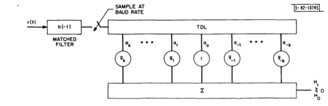
Recalling our discussion in Sec. A on the generation of the sufficient statistics ak, it is clear that the decision rule (26) may be implemented as shown in Fig. 7, where the weights gk are seen to appear as gains on the TDL taps. This structure will be referred to as the "conventional" equalizer throughout the remainder of the report, to distinguish it from the "decision-feedback" equalizer to be derived and studied later. Further, it will prove convenient in the following discussions to denote the tap gains as a vector, defined by
14 g2
(27)
which we will frequently refer to as the "tap-gain" vector.
The conventional equalizer structure with its gains as defined by Eq. (25) is, of course, only optimal under Assumption (4), hence sub-optimal for the actual binary signaling problem of in-terest. We would like, therefore, to next adopt this sub-optimal receiver structure, but to abandon Eq. (25) and to determine a tap-gain vector g more appropriate for the present problem.
SAMPLE AT Ix- as- n?4l
MATCHED FILTER
Ht
< o
Ho
v
Fig. 7. Structure of conventional equalizer.
At this point, we would like to determine those tap-gain settings which optimize the equalizer performance, minimizing its probability of error. For the special case where the sum of the sidelobe magnitudes is less than unity, Aaron and Tufts 3 have done this by first minimizing the output noise variance for a given set of sidelobes, and then working through a specific example, employing a search in tap-gain space to arrive at those settings which minimize the probability of error. This approach was feasible only because they consider small numbers of sidelobes and taps, thus requiring summation over only a small number of possible message sequences. In realistic applications, as we discuss further in Sec. IV, the number of terms involved in such
a probability-of-error computation becomes prohibitively large, and we therefore must be con-tent with some other method, and with less-than-optimal tap-gain settings.
Instead of attempting to minimize the probability of error directly, authors usually attempt to minimize the intersymbol interference appearing at the receiver output. Two distortion measures are currently in use. With the mainlobe assumed unity, and the summations over the sidelobes, these measures are
D = 0LE qi (28) 15 ____ _1111-1- .1--. -.-.--- --- --A 9 90 91
and
D:=
qil
(29)
where the qi are the output sidelobes resulting from a single pulse transmission, as shown in Fig. 8. DiToro uses the Da criterion in his ADAPTICOM receiver, while Lucky
9 '
uses the D: criterion, although he asserts there is probably little difference in terms of performance using either criterion. In this report, we adopt a modified Da criterion under which we include the additive noise appearing at the output, and find those tap-gain settings which minimize the total output distortion.
qn 13- 42- 107461
q-2
i
T
2
I
Fig. 8. Typical output sidelobes from conventional equalizer for qI a single to = +1 pulse transmission.
T
q2-
T t
- M 1 1 M
-M qM
We first determine an expression for the output distortion in terms of the TDL gains. For a single 0 = 1 transmitted pulse, synchronous sampling of the matched filter output renders a sequence of samples
zk z(kT)= 5 r(t) h(t + kT) dt
S
[h(t) + n(t)] h(t + kT) dt = Pk + Wk (30)where we have defined
k :
5
h(t) h(t + kT) dt (31)and
wk = n(t) h(t + kT) dt .(32)
The TDL output is then a sequence of samples given by the convolution of the zk sequence with the tap-gain vector g:
Z
k-mgm= £ k-mgm + E Wk-mgmm m m
qk + k (33)
where we have defined the first sum on the right-hand side to be qk, and the last sum to be nk, as indicated. In transmitting an infinite sequence of pulses modulated by the k (which we have previously assumed to be independent, of unit variance, and zero mean), the output distortion at any sample time, say, the zeroth sample time, will be given by:
2 2 2
Output distortion = q-q 0 + no . (34)
k
16
Normalizing the tap gains such that q = 1, then to minimize the average output distortion, we must minimize the quantity
2
+ n 2(35)
qk +no kFrom the definition of the qk in Eq. (33), we find that
q2=
k
, (= Pk-mgm) (Z k-vgv) q-(Z
· ,kmm
(z
(k-vgv) k k m v =Z gm( Pk-mPk-v) gv (36) m v k and no= Wmgm( W-vgv) m v=
Z Z
gmW _wmw _vgv m v N gg y(37)~-
NO gmPm_vgv m vthe latter step holding since, from Eqs. (31) and (32), it follows that w_mw =
5
h(t- mT) h( -vT) n(t) n(T) dT dt2 NOPmv (38)
If we define matrices X and Y by their elements
Xmv = Pk-mPk-v (39)
k and
Y mv =P m-v
n-v
(40)then substituting these into Eqs. (36) and (37), using the tap-gain vector notation g defined in Eq. (27), we may write Eq. (35) as
g Xg+ NgTyg gTX + 2 NoY]g (41)
Under the constraint that the mainlobe is unity, which we may write as
T T
g S° = _ = 1 (42)
where we have defined the column vector
17
---1
(P0
'P
(43)
then our problem is to minimize Eq. (40) subject to the constraint Eq. (41). Introducing the Lagrange multiplier , we may do this by minimizing the quantity
J A gT[X + 2 NoY] g + (gTS° -1)
in order to find the tap-gain vector g which is optimal under our distortion criterion. It is straightforward to show that
A
aJ
ag
L
1 =[X + 1 NOY] g + Opand, further, that aJ/ag is zero for
[X + NY] 1 (
g= o [X NOY] _
(44)
(45)
(46)
where Eq. (42) has been used to determine and replace A.
Equation (46) is the desired solution, We next verify that it exists, is unique, and renders a minimum of Eq. (44). Since the output sample variance is always non-negative, and clearly zero only if we turn the TDL off completely by setting g = 0 (for otherwise some noise at least would appear at the output), then it follows from Eq. (41) that the matrix
18
1
X+ 2 N Y0- (47)
is positive definite, and its inverse exists (Ref. 14, p. 46). Since the inverse of a matrix is itself unique, it follows that the solution Eq. (46) exists and is unique. Moreover, the facts that
2
= 2[X + NY
2 -- 2
oY-and that the matrix of (47) is positive definite, are sufficient conditions to guarantee that our solution Eq. (46) does indeed render a minimum of Eq. (44) (see Ref. 15, p. 227).
Having thus arrived at the tap-gain settings which minimize the total distortion at the output, we next want to determine their asymptotic behavior as the length of the TDL becomes arbitrarily large. We define a unity vector u:
0 0 1 0 0 (49) Noting that (YU)k = m km m =kO and (50) (48) (YY)mv= Z YmkYkv = k k '°m-k~°k-v = Xmv (51) (52) then, asymptotically, we may write
Yu= p Y 1= = u
and
YY= X (53)
Using Eqs. (52) and (53) in Eq. (46), and ignoring for the moment the denominator which is merely the normalization, we find asymptotically the solution
g = [YY + 1 No] - = [Y+ I] 1 u (54)
We next want to study this asymptotic result still further. Rewriting Eq. (54) in terms of a sum-mation, we have
[Pi-j + 2 N 6ij] gj= 6i0 (55)
J
Subtracting the j = 0 term from both sides, and normalizing the tap-gain vector such that gO = 1, we find the tap gains must satisfy
1
['i-j + 2 No06ij gj = 'i (56)
j#0
for all i
#
0. Dividing through by No, and noting by comparison of Eqs. (8) and (31) that i/No = bi, then Eq. (56) becomes[bi
j + 6ij] gj = -bi i 0 . (57)jW0
But, from Eq. (19) we observe that ci = b. for i f 0, and from Eq. (20) that b.i + (1/2) 6ij = Qij;
hence, Eq. (57) is seen to be identical to Eq. (25). Thus, we have shown that the tap gains min-imizing the total output distortion of the conventional equalizer are asymptotically the same as the tap gains obtained for the optimal receiver which was designed assuming that the interference from other bauds was Gaussian, as the length of the TDL becomes arbitrarily large.
Next, we observe that Eq. (54) may be written as
[Y + 2 NoI] g = (58)
From Eq. (40) we note that Y is a Toeplitz matrix, since the elements along any of its diagonals are the same, Yij = Yi+ ,j+t (see, for example, Ref. 16). Thus, asymptotically, Eq. (58) be-comes equivalent to convolving the row vector
uT[Y + NoI] (59)
with the tap-gain vector g to obtain the vector u. Therefore, this may be written as a set of equations
£'
['k-m + 2 N0Uk-m] gm Uk (60)m
Further, by defining transforms
G(w)
£
gm e-mw (61) me(w)
r<P_
eJ-ljCMW (62) m and U(w)9 Umu e- jm W = (63) m 20it follows that we may solve Eq. (60) by first setting
G(co) =1 (64)
4(w) + - N0
and then inverse transforming to obtain the tap-gain vector components
gm= G(w) ejm dco (65)
The relation Eq. (64) was obtained previously by George,17 except for an arbitrary gain factor he incurs by neglecting normalization. George arrived at this relation somewhat more directly by starting out initially with an unconstrained linear receiver. Later, Collt 8 adopted the re-sulting conventional receiver structure and, using a variational approach as George had done, determined the tap-gain equations for minimizing the output distortion for TDL of finite length. Our formulation led directly to the solution for TDL of finite length, and then asymptotically to George's result. The approach we present here enabled us to establish the existence and unique-ness of the solution, and to relate it asymptotically with the tap gains obtained in our original derivation of the conventional equalizer structure.
As explained in the Introduction of Sec. I, we will study the performance of the sub-optimal conventional equalizer in detail in Sec. IV, but first, in Sec. III we will consider another sub-optimal receiver - the decision-feedback equalizer.
21
III. EQUALIZATION USING DECISION FEEDBACK
We saw in Sec. I that previous applications of decision feedback in equalization have been concerned, indirectly at least, with effectively measuring the equivalent channel in order to achieve tap-gain settings for the conventional equalizer we derived in Sec. II or its cascade equivalent. Next we derive a new equalizer structure in which the decision feedback plays a different role. We then optimize the parameters of this new structure and, finally, we briefly
compare its sidelobe suppression properties with those of the conventional equalizer.
Our problem is the same as that stated in Sec. II, namely, to decide between the hypotheses Hi and H0 that
40
is +1 or -1, respectively, given a receiver inputr(t)= E kh(t - kT) + n(t) . (66)
k Now, under the assumptions:
(1) k are independent,
(2) H and Hi are equally likely, and
(3) n(t) is white Gaussian noise, of double-sided spectral height N0/2,
we found the optimal equalizer structure of Fig. 6. We now make two additional assumptions which will lead us to a sub-optimal receiver structure:
(4) k are Gaussian random variables of zero mean and unit variance for k > 0, and
(5) Ok are known for k < 0 (i.e., error-free decision feedback).
As we observed in making a similar assumption in Sec. II, Assumption (4) renders our model inaccurate for binary AM or PSK systems in which k = +1 or -1 for all k, while Assumption (5) is valid for decision-feedback equalizers only in the absence of decision errors.
Under our Assumption (5) that , as defined earlier by Eq. (3), is known correctly via decision feedback, the optimal receiver computes the likelihood ratio
p[r(t)l -, 0 =1] A = p[r(t)l -,
0
=-1
Sp[r(t)l -0 ' t ] p(+) d + =1 (67) f p[r(t)l 0, , ] p( ) dl _ (67)We found earlier in Eq. (6) that we could write
p[r(t)l 0,i,] = K1 exp[I, kak - ijbi b-j] (68)
i j
where the ak and bk are defined in Eqs. (7) and (8), respectively. Ignoring constant factors
in-dependent of + and the value of 0 which will come outside the integrals in Eq. (67) and cancel each other out, we may rewrite the right-hand side of Eq. (68) as
23
"I'-""`-exp [Oa0
+ma m
kmb k-m
k2
m>0 k<0 m>0
-2~o Z kbk -2tOZ mbm -
3
ijmb j-m (69)k<0 m>0 j>0 m>O
Now, under Assumption (4), we may write
p(+) = K2 exp -2 [ m =K2 exp - 2 .j jmm0 7
m>0 j>0 m>0
Thus, by combining Eqs. (69) and (70), the numerator of Eq. (67) may be written as exp 0a0 - 2 4o Z 4kbk exp-
Z Z
j(bjm + 2 6jm) mk<O j>0 m>0
+ 2 m( - bkm - -- b)j d) (71)
m>O k<O k0=1
By completing the square in the exponent of the integrand of Eq. (71), it is straightforward to show that this numerator of A is
exp [ 0a0-2 0 kbkZ k b
+
(2
aj- bj kk- b) Pjk<0 j>0 m>0 k<0
(
m Z bm-4
-0 m
|
(72)n<O 0
where the Pjm are the elements of the matrix P defined by
PA R-1 (73)
and where we have defined the matrix R via
R.= b. + 2 6. jm > 0 (74)
jm J-m 2 jm
Note that, except for the ranges of their subscripts, the matrix R defined by Eq. (74) and the matrix Q defined by Eq. (20) are otherwise identical. Since Eq. (72) evaluated at 40 =
-1
renders the denominator of Eq. (67), it is seen that the optimal receiver, under our assumptions, computes
A = exp 2a0-4 bkk-4 m b
[m
a[ - bk_-jk) Pjmj (75)k<0 m>O j>O k<O
If we define
9 Z P jm bm (76)
g jm
m>O
fkA 2bk + 2 gjbj k (77)
j>o
then the decision rule of Eq. (14) becomes Hi
a0+ gjaj-
Z
fk0k (78)j>O k<O H0
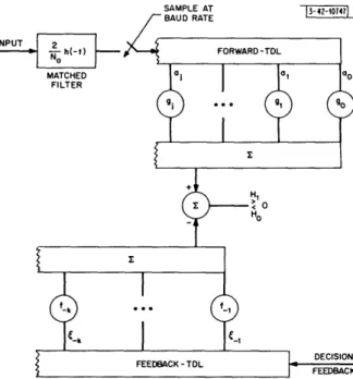
As shown in Sec. II [see Fig. 4(b)], the a are sufficient statistics which may be generated by matched filtering to the equivalent channel, sampling the output synchronously at the baud rate, and passing the samples into a TDL. Note, however, that with the present sub-optimal equal-izer, only the a for j > O0 enter into the decision rule, just as we noted is true of the optimal equalizer whenever the previously received baud modulations k are known. Whereas the effects of these earlier-baud ~k were accounted for in the optimal equalizer structure by the C(s) con-stants of Eq. (13), which themselves undergo nonlinear operations before effecting the output, they enter in this sub-optimal equalizer as a weighted sum, the second term of Eq. (78). Thus, the overall decision rule of this sub-optimal receiver may be implemented as shown in Fig. 9.
SAMPLE AT
13-47-047-INPUT
Fig. 9. Structure of decision-feedback equalizer.
It is seen to consist of a forward-TDL, which weights the sufficient statistics a by the tap gains gj for j > 0, where we have defined g 1, and of a feedback-TDL through which we must pass
the k upon which decisions previously have been made, where they are then weighted by the tap gains fk'
As discussed in Sec. II when considering the conventional equalizer, the tap gains as defined by Eqs. (76) and (77) are only optimal under the assumption of Gaussian interference from future bauds. Thus, as before, we now want to adopt the equalizer structure of Fig. 9 and determine those forward- and feedback-TDL tap gains that minimize the total distortion appearing at the output in the absence of decision errors. We first introduce some additional definitions that will prove useful in the following discussion:
25
-q = signal component of the forward-TDL output at the mth sample
time, when a single ~0 = +1 baud is transmitted (79)
qk = f h(t) h(t + kTb) dt = sampled channel autocorrelation
function at = kTb (80)
Y = matrix with elements Yjk = '°j-k for j, k > 0 (81)
X = matrix with elements Xjk = q'Pj+m 4Pk+m for j, k 0 (82)
m<O
cp = column vector with elements qPi for i 0 (83)
g = column vector with elements gi for i 0 (84)
f = column vector with elements f. for i 1 (8 5)
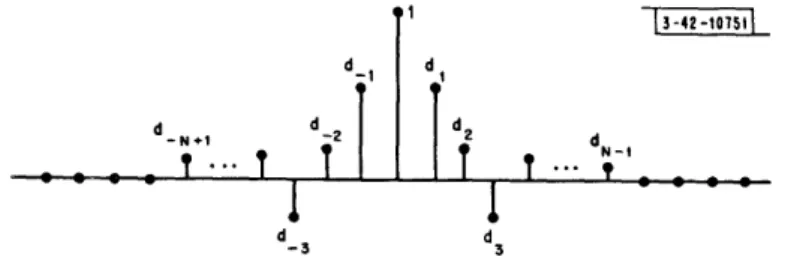
A typical response of the decision-feedback equalizer to a single transmitted baud of 0 = +1 is shown in Fig. 10. It is always an asymmetrical waveform, having M more samples occurring
before the main sample (which is denoted sample qo 113-42-s07481 number 0) than after it, where the MF output has
q ' ' 2M + 1 nonzero samples. This is in contrast with
the typical output from the conventional MF-TDL equalizer, which was seen in Fig. 8 to always
ex-9" -2 ? Thibit symmetry about the main sample.
Before we can proceed to determine the optimum choices of g and f under our
minimum-output-q3
sample-variance criterion, we must first
under-Fig. 10. Typical output sidelobes from decision- stand the effect of the decision feedback on the feedback equalizer for a single 0 = +1 pulse output distortion. Consider the signal component
transmission. out of the forward-TDL at the first sample time:
gj[aj+]signal gj[N kh(t - kTb) {ht (j + ) T dt (86)
j>O j>0 k
The contribution to this component, which is due to the bauds for which decisions have already been made (that is, on all the k up to and including 0), is then
2
£
gjbj+ _kk (87)j>O k0
Next, consider the output of the feedback-TDL at this same first sample time. With the use of Eq. (77) for the fk' this becomes
Z
fktk+1 = 2 [bk+
gi.b-]
k+1 (88)k<O k<0 j>0
and, if we let k* = k + 1,
£
kk+1 2£
fbk,,- + gjibj+lk . k*k<O k*<O j>O
2 E gjbj+l-k* .k* (89)
j>0O k*.O
Here, we have used bk*,1 = bi k* and our earlier definition, go A 1. Thus, we see from
comparing Eqs. (87) and (89) that in the absence of decision errors the feedback-TDL output is exactly the same as the contribution to the forward-TDL output at the first sample time, attrib-utable to past bauds, hence, there is no net contribution to the distortion from those bauds upon
which decisions have already been made.
In abandoning Eqs. (76) and (77) in order to optimize the tap gains under a minimum-output-distortion criterion, we wish to retain the nature and purpose of the feedback-TDL as seen above with the optimal solution - namely, to cancel out sidelobes attributable to past bauds. In the absence of decision errors, then, with the feedback-TDL tap-gain vector f suitably chosen, it
is clear that the output distortion we want to minimize is given by
£
qm + output noise variance (90)m<O
Under the constraint that the main sample be unity, we may include q0 in the summation to find
that
, qm= , , gjXjkgk = g (91)
m(0 j) kO
while the output noise variance can be found, as in Eq. (37), to be
2 gjYjkgk = Y Yg (92)
j) kO
Thus, under the constraint of Eq. (42) that the mainlobe be unity, we proceed as in Sec. II to minimize the quantity
J=gT[x+ YJ g + x( gT ) (93)
over the choice of the forward-TDL gain vector g. The unique solution is again given by
X + NO Y _p
g (94)
TIX+ - 2Y _
This result appears formally identical with that obtained for the conventional equalizer, Eq. (46). The differences are in that we have redefined the vector qo and the matrices X and Y in Defi-nitions (81), (82), and (83), and now their subscript ranges differ from the ranges used in study-ing the conventional equalizer. Thus, while (p was symmetrical and X Toeplitz for the conven-tional equalizer, these properties do not hold for the _o and X for the decision-feedback
27
equalizer. Both of these differences result from the fact that sidelobes occurring after the mainlobe are ignored in the decision-feedback equalizer. In Definition (82), for example, this is reflected in that the summation is restricted to m < 0, whereas the corresponding summation Eq. (39) of the conventional equalizer has no such restriction.
The proper choice of the f vector now follows directly from Eq. (77), except that we have dropped the 2/N 0 factor common to the terms of Eq. (78) (that is, the aj contained this factor,
while it has not been included in the MF output in the present discussion), and thus the 2bk be-come replaced by the cok of Definition (80):
fk = gjOj-k for k < 0 (95)
j>0
If we define a matrix Y with elements
Yjk = j-k for
jk < 0 (96)
[note that it is the range of k which distinguishes this matrix from the Y matrix of Definition (81)], then the feedback-TDL tap-gain vector may be conveniently written as
f = g (97)
Thus, once the sampled channel autocorrelation function and the additive noise level have been specified, we can use Eqs. (94) and (97) to determine the tap gains of the minimum-output-distortion decision-feedback equalizer. Moreover, using the same arguments we presented for the conventional equalizer, we can show that the solutions to these equations exist, are unique, and render a minimum of Eq. (90).
We want next to compare the operation of the decision-feedback equalizer of Fig. 9 with that of the conventional equalizer structure shown in Fig. 7. Since in actual implementation,
equal-izer cost is directly related to the number of delay elements and amplifiers required, then our comparisons will be based on equalizers having the same number of taps. The conventional equalizer, of course, uses its allotment of taps on its single TDL, while the decision-feedback equalizer must devote part of its taps to the feedback-TDL and the remainder to the forward-TDL.
Before proceeding, we want to consider the number of taps required on the feedback-TDL. We may rewrite Eq. (95) as
f-k = Pmgm-k for k > 0 (98)
m>-k
and thus, for a channel where the maximal dispersion is over, say, N bauds (that is, where 0on
=
0 for n > N), then from Definition (83) it is clear that
f for all k > N (99)
Thus, at most, N - 1 taps are required in the feedback-TDL of the decision-feedback equalizer, and any additional taps which are available may be employed in the forward-TDL.
The sampled MF output for a single pulse transmitted is always symmetrical, thus it follows from Eq. (38) that a conventional equalizer having an odd number of taps always has a symmetri-cal tap-gain vector. Hence, a (2M + )-tap conventional equalizer really has only M degrees of
Ad L5-42-1o?4.] freedom, assuming that the centertap gain is 0~~~~~~f-zils
normalized to unity. With these M degrees of freedom, the conventional equalizer must si-multaneously attempt to suppress the sidelobes attributable to both past and future baud trans-missions. On the other hand, as' we noted above, the decision-feedback equalizer feedback-TDL requires only N - 1 taps for a channel with a Fig. 11. Example sampled channel autocorrelation
function for illustrating sidelobe suppression in con- maximal dispersion of N bauds, leaving 2 ventional and decision-feedback equalizers. 2 - N taps and degrees of freedom available for
the forward-TDL. Moreover, the forward-TDL
gains are computed without regard to the qm for m > 0, and only the qm for m < 0 are taken into account (see Fig. 10). Thus, the forward-TDL need only be concerned with suppressing the sidelobes attributable to future bauds, that is, those bauds upon which decisions have not yet been made.
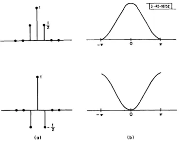
To illustrate the advantages resulting from the greater degrees of freedom available to the decision-feedback equalizer, we will consider the sampled channel autocorrelation function shown in Fig. 11. Using a 21-tap TDL in the conventional equalizer, with the tap gains given by Eq. (46), the tap-gain vector has a limiting solution with increasing SNR and, accordingly, there is a limiting sidelobe behavior at the output
13-2-4o1sol
for a single pulse transmission, as shown in Fig. 12(a). The forward-TDL output of the equiv-alent decision-feedback equalizer, with its tap gains computed according to Eq. (94), is shown in Fig. 12(b). In this example, the conventional equalizer has M = 10 degrees of freedom com-pared with 2M + 2 - N = 17 degrees of freedom available to the forward-TDL of the
decision-feedback equalizer. The resulting sidelobes qm I I I I I I
for m < 0 for the decision-feedback equalizer are
seen to be considerably smaller under either a CONVENTIONAL EQUALIZER
(a) CONVENTIONAL EQUALIZER Da or D distortion criterion [defined in Eqs. (28)
and (29), respectively] than are the sidelobes of the conventional equalizer. As we discuss fur-ther in Secs. IV, V, and VI, this greater sidelobe-suppression behavior results in a large improve-ment in the performance of the decision-feedback equalizer over that of the conventional equalizer. As expected, the sidelobes qm for m > 0 at the output of the decision-feedback equalizer forward-TDL are very large, since they were not involved in the tap-gain optimization. In the absence of
(b) DECISION-FEEDBACK EQUALIZER decision errors, these large sidelobes are
ex-Fig. 12(a-b). Limiting sidelobes with increasing
actly subtracted out by the feedback-TDL com- SNR of 21-tap conventional and decision-feedback
ponent of the output, as we observed previously. equalizers, applied to channel of Fig. 11.
29