Deep Learning for Sentiment and Event-driven REIT
Price Dynamics
by
Yao Zhao
B.Eng., Tsinghua University (2016)
M.Sc., London School of Economics (2017)
Submitted to the Department of Urban Studies and Planning and the
Department of Electrical Engineering and Computer Science
in partial fulfillment of the requirements for the degrees of
Master in City Planning
and
Master of Science in Electrical Engineering and Computer Science
at the
MASSACHUSETTS INSTITUTE OF TECHNOLOGY
February 2020
c
○2020 Yao Zhao. All Rights Reserved
The author here by grants to MIT the permission to reproduce and to
distribute publicly paper and electronic copies of the thesis document in
whole or in part in any medium now known or hereafter created.
Author . . . .
Department of Urban Studies and Planning
Department of Electrical Engineering and Computer Science
January 16, 2020
Certified by . . . .
David Geltner
Professor of Real Estate Finance
Thesis Supervisor
Accepted by . . . .
Ceasar McDowell
Professor of the Practice
Chair, MCP Committee
Department of Urban Studies and Planning
Accepted by . . . .
Leslie A. Kolodziejski
Chair, Department Committee on Graduate Students
Deep Learning for Sentiment and Event-driven REIT Price
Dynamics
by
Yao Zhao
Submitted to the Department of Urban Studies and Planning and the Department of Electrical Engineering and Computer Science
on January 16, 2020, in partial fulfillment of the requirements for the degrees of
Master in City Planning and
Master of Science in Electrical Engineering and Computer Science
Abstract
This research aims to figure out how textual information in the real estate news can be applied to predicting the price dynamics of REIT (real estate investment trust), a publicly traded security in the exchange whose income is backed up by real es-tate. Due to the information gap in the market and the sentiment-induced irrational trading behaviors, the market often witnesses the departure of REIT price from its fundamental NAV (net asset value). Traditional REIT pricing models fail to incorpo-rate these behavioral factors and the real time market information, leading to a gap in current empirical studies. With the development of deep learning and natural lan-guage processing (NLP) techniques, we are curious about how to properly represent and extract textual information in the real estate news, in a way that allows us to capture the up-to-date market events and irrational sentiment, and incorporate them in REIT pricing.
To achieve this goal, I conduct a two-stage analysis. In the first stage, I focus on two NLP tasks, including the sentiment analysis and event extraction. On the end of sentiment analysis, I construct several sentiment measures based on the traditional textual analysis methods. Besides, I train and obtain the sentiment-specific word em-beddings on a human-labeled financial news corpus. One the event extraction end, two approaches of event representations are used, which separately corresponds to an un-supervised and a un-supervised learning model. First, I represent an event as a structured triplet 𝐸 = (𝑂𝑏𝑗𝑒𝑐𝑡1, 𝑃 𝑟𝑒𝑑𝑖𝑐𝑎𝑡𝑒, 𝑂𝑏𝑗𝑒𝑐𝑡2), and use an unsupervised NTN (neural
ten-sor network) model to obtain the event embeddings. Second, I follow a supervised model to represent the event in the form of 𝐸 = (𝑡𝑟𝑖𝑔𝑔𝑒𝑟, 𝑎𝑟𝑔𝑢𝑚𝑒𝑛𝑡1, 𝑎𝑟𝑔𝑢𝑚𝑒𝑛𝑡2, ...),
and fine-tune a BERT model on the event extraction task.
In the second stage, with the help of the sentiment measures, sentiment-specific word embeddings and the pre-trained event embeddings, I implement and compare several deep learning models for REIT price prediction. The best-performing NTN+CNN
model greatly outperforms the traditional ARIMA model, in that it decreases the MSE loss by around two thirds, and increases the classification accuracy of price movement by around 8%. The VAR analysis indicates that positive market sentiment granger-causes the REIT price change between 2011 and 2018, while the negative sen-timent has no significant effect on the market.
Thesis Supervisor: David Geltner Title: Professor of Real Estate Finance
Acknowledgments
The chapter 6 of this thesis, Supervised Learning: Event Identification and Classifi-cation, is revised from my 6.867 course project, which is jointly done by Haowei Xu and me. Besides, I would like to take this opportunity to thank all my professors and friends for their support during my study at MIT.
Contents
1 Introduction 15
2 Literature Review: REIT Pricing 23
2.1 The deviation of REIT prices from NAV . . . 23
2.1.1 Information Gap . . . 24
2.1.2 Sentiment-induced Trading Behavior . . . 25
2.1.3 Stock Market Dynamics . . . 26
2.2 Evidence on the Irrational Factors in the REIT Market . . . 27
3 Literature Review: NLP and Deep Learning for Market Prediction 29 3.1 NLP for Stock Price Prediction . . . 29
3.2 Word, Event and Paragraph Embeddings . . . 30
3.2.1 Word Embeddings . . . 31
3.2.2 Event Representation and Embeddings . . . 32
3.2.3 Paragraph Embeddings . . . 36
4 Data and Models 37 4.1 Data . . . 37 4.1.1 Textual Data . . . 38 4.1.2 Numerical Data . . . 45 4.1.3 Fama-French Factors . . . 48 4.1.4 Growth Opportunities . . . 48 4.2 Exploratory Analysis . . . 49
4.3 REIT Pricing Models . . . 53
4.3.1 Time Series Analysis . . . 54
4.3.2 Big Picture: Deep Learning Task - Incorporating both Textual and Numerical Information . . . 55
5 Sentiment Analysis and Unsupervised Event Extraction and Embed-dings 57 5.1 Sentiment Analysis . . . 57
5.1.1 Textual Analysis . . . 57
5.1.2 Supervised Training . . . 59
5.2 Event Extraction . . . 66
5.3 Unsupervised Event Embeddings . . . 68
5.3.1 Word2Vec on Factiva Real Estate Corpus . . . 68
5.3.2 Unsupervised Learning: Neural Tensor Network . . . 70
6 Supervised Learning: Event Identification and Classification 73 6.1 Task Description . . . 73
6.2 Approach . . . 74
6.2.1 Bi-LSTM . . . 75
6.2.2 BERT . . . 75
6.2.3 CRF . . . 76
6.2.4 Evaluation metrics: F1-score . . . 77
6.3 Experiments . . . 77 6.3.1 Baseline model . . . 78 6.3.2 Trigger extraction . . . 79 6.3.3 Argument identification . . . 86 6.4 Conclusions . . . 89 7 Empirical Results 91 7.1 Time Series Analysis . . . 91
7.1.2 VAR Models . . . 98 7.2 NTN+CNN Models . . . 103
List of Figures
1-1 The trend of real estate media sentiment and REIT return. . . 16
3-1 C&W model. . . 31
3-2 The event role mapping theory. . . 33
4-1 The number of news in each year. . . 38
4-2 An example of the Factiva database. . . 39
4-3 An example of the Factiva database. . . 40
4-4 Trend of the REIT index (Wilshire US REIT). . . 45
4-5 The NAV premium. . . 46
4-6 The NAV premium betwen 2009 and 2018. . . 47
4-7 Comparing the trend of REIT index and NAV. . . 47
4-8 The first order difference of REIT Index. . . 49
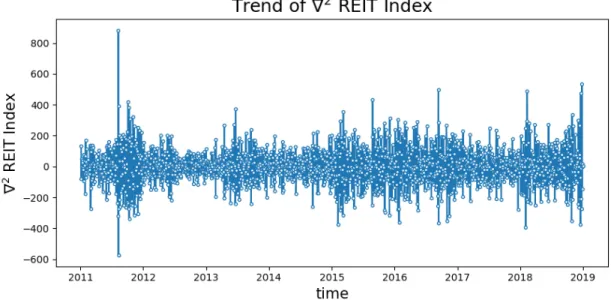
4-9 The second order difference of REIT Index. . . 50
4-10 The ACF estimate of the first-order differenced REIT index.. . . 52
4-11 The ACF estimate of the second-order differenced REIT index. . . 52
4-12 The PACF estimate of the first-order differenced REIT index. . . 53
4-13 The PACF estimate of the second-order differenced REIT index. . . . 53
4-14 The deep learning architecture for REIT pricing. . . 56
5-1 Correlation matrix of different sentiment measures. . . 59
5-2 Comparing different sentiment measures. . . 59
5-3 Frequent words in the Financial PhraseBank. . . 60
5-5 Sentiment Specific Word Embeddings (SSWE). . . 61
5-6 Model for pre-training SSWE. . . 62
5-7 Training history of the SSWE model. . . 64
5-8 Visualizing the SSWE results. . . 64
5-9 The neural tensor network for event embeddings. . . 70
6-1 An example of the ACE 2005 data. . . 74
6-2 Graphical structure of a linear CRF. . . 76
6-3 The neural network structure used across all models. . . 80
6-4 Evaluating different ways of treating the No-trigger sentences. . . 82
6-5 Conditional probability model. . . 83
6-6 Visualization of the word embeddings. . . 85
6-7 The training curve for the argument identification task with different word embedding schemes. . . 87
6-8 Trigger classification and argument identification on an example. . . . 89
7-1 ARIMA(1,2,2) fitting of the training data. . . 94
7-2 ARIMA(1,2,2) prediction of the REIT index movement. . . 94
7-3 ARIMA(1,2,1) fitting of the training data, with exogenous variables. . 97
7-4 ARIMA(1,2,1) prediction of the REIT index movement, with exoge-nous variables. . . 97
7-5 VAR fitting of the training data. . . 102
7-6 VAR prediction of the REIT index movement. . . 102
7-7 The architecture of NTN+CNN model. . . 103
List of Tables
4.1 Sentiment distribution of sentences in Financial PhraseBank. . . 41
4.2 Trigger statistics of ACE 2005 corpus. . . 42
4.3 Class statistics of ACE 2005 corpus. . . 42
5.1 Model setting of the sentiment classification. . . 63
5.2 Testing the sentiment classification accuracy. . . 65
6.1 The performance of models on the trigger identification and classifica-tion task. . . 81
6.2 The F1-scores for the argument extraction task with different word embedding scheme. . . 88
Chapter 1
Introduction
The United States witnessed an overwhelming housing bust following a great boom in the last decade. Originating from the subprime crisis, the 2008 recession led to soaring unemployment rates, countless bankrupts and tremendous GDP loss. Case et al. (2012) report that people’s expectation on the real estate market reached an ab-normally high level at the peak of the boom, while the crisis following the downward turning point was closely associated with the changing market expectation. Since the real estate market is vulnerable to irrational factors and speculative bubbles (Case and Shiller, 1988; Walker, 2014; Ling and Naranjo, 2015; Soo, 2018), market predic-tion and early warnings are necessary.
But can we predict the market dynamics? The efficient market hypothesis (Fama, 1965) seems to discourage us, because it assumes all available information has been incorporated into the current asset price, and accordingly, stock price should depend on fundamentals only. However, a number of behavioral finance studies report as-set pricing anomalies, suggesting that fundamentals are not sufficient to explain the stock price variation (Shiller, 1980; Summers, 1986; Zhong et al., 2003; Barberis et al., 2005). On one hand, the market seems unable to completely absorb new information in a real-time manner. The influence of new market events could last for a period of time, ranging from one day to several months (Tetlock et al., 2008; Bengio et al., 2009; Xie et al., 2013; Ding et al., 2014). On the other hand, the investor sentiment has been identified as another important factor in asset pricing, which is broadly
defined as a belief about future market returns that are not justified by any fact at hand (DeLong, 1990; Baker and Wurgler, 2007; Tetlock, 2007; Soo, 2018).
This research will focus on the real estate investment trust (REIT), a special security that enables investors to engage in the expensive real estate investment by purchas-ing shares of real estate portfolios. The properties in a REIT portfolio are called its underlying properties, in the sense that the dividends of REIT are inherited from the operating income of these properties, together with risks and market expectations. Since REIT is listed in the exchange, it enjoys greater liquidity than its underlying properties. Therefore, the price of REIT should incorporate both up-to-date pricing information and irrational factors much quicker. This suggests it should be of signif-icance to predict the REIT price dynamics, to meet the goal of market monitoring.
Figure 1-1: The trend of real estate media sentiment and REIT return. Figure 1-1 presents an anecdotal evidence for the importance of predicting REIT dynamics. It shows a lead-lag pattern between REIT return and the real estate senti-ment index constructed by Ruscheinsky (2018). Clearly, in the last housing cycle, the turning point of the real estate media sentiment (marked in blue) appeared several months before that of the REIT return (marked in red), for both collapse and
recov-ery. Specifically, the REIT return started to decline around January 2007, while the market sentiment had already begun moving downward since half a year ago. This is in line with Case et al. (2012)’s survey, which indicates that the change of people’s expectation led that of property price. These studies seem to implicitly support the possibility of predicting the REIT price movement.
However, previous studies rarely define sentiment precisely, leaving it difficult to make clear distinctions between the sentiment backed up by new market information and the purely irrational expectations. Intuitively, bull/bear news that release new mar-ket events could trigger positive/negative sentiment, and they should certainly follow a different process from the completely irrational sentiment. To this end, it’s neces-sary to figure out whether a price change is driven by real-time market information or irrational sentiment, and to infer how much of the REIT price could be backed up by up-to-date information (i.e. updated fundamentals), and how much it is biased by irrational factors. To fulfill this goal, we need to properly capture both real-time market information and the irrational sentiment.
This research will incorporate both numerical and textual information available in the real estate market. In general, I set up deep learning models with the Long-short Term Memory (LSTM) or Convolutional Neural Network (CNN) structure, to estimate the dynamics of the U.S. REIT index. Both CNN and LSTM are reported to perform well in time series prediction. Numerical information used in this research includes market fundamentals, such as the Net Asset Value (NAV) and the Fama–French factors. For textual information, I employ the Natural Language Processing (NLP) techniques to extract real-time information from the real estate news, as suggested by many previ-ous stock prediction studies (Das and Chen, 2007; Tetlock, 2007; Tetlock et al., 2008; Ding et al., 2014; Akita et al., 2016). A glance at the real estate headlines would give us some intuition about what to extract.
Below I list several examples retrieved from the Reuters.
Headline 1: Chinese may soon park money in U.S. buildings, Jul 01 2005 Event: More Chinese investors are investing in the U.S. real estate market
Sentiment: Positive
Headline 2: Raw materials weigh on U.S. builders, developers, Jul 01 2005 Event: Rising price of raw materials makes developers suffer
Sentiment: Negative
Headline 3: Housing executives see U.S. price drop, not crash, Jul 01 2005 Event: None
Sentiment: Negative
Headline 4: Toll Brothers studying possible expansion abroad, Jul 01 2005 Event: A real estate company plans to expand
Sentiment: Neutral
The headline samples above indicate that market events and sentiment are two pos-sible layers of information we could extract from the news, though they are not necessarily orthogonal to each other. On one hand, news reveals up-to-date events in the real estate market, including housing policy, demand and supply change, con-struction cost, the real estate company’s management strategy, etc. Events can be at either the nation, city, or company level, and their impacts can be short-term and/or long-term. To extract these market events, analyzing the syntactic context of news becomes important. On the other hand, news, especially market reviews written by real estate specialists, can spread strong market sentiment to investors. Accordingly, our task is to identify those specific words with strong sentiment in the news context, such as collapse, crash, boom, soar, etc. Usually, these reviews reveal no additional market information, but they are super powerful in affecting people’s expectation and triggering irrational trading behavior.
How to extract events and sentiment from real estate market news and properly repre-sent them? Considering that the extracted news reprerepre-sentation will serve as an input for the deep learning model, it’s necessary to encode them as fixed-length vectors. For
sentiment analysis, our objective is to first learn the continuous, sentiment-specific representation for each word (i.e. word embeddings), and then apply a convolutional or recurrent layer to compose a sentiment-specific vector representation for each head-line, whose length should be fixed. Given that the unsupervised learning algorithms for word embeddings focus mainly on the distributional properties of words but ig-nore their semantic meanings, I switch to a supervised method, Sentiment Specific Word Embedding (SSWE) (Tang et al., 2014). By incorporating the human-labeled sentiment polarity of headlines in the loss function used for training, this model is expected to return word embeddings which carry sentiment information.
For market events, this research mainly adopts two approaches. First, I follow Ding et al. (2014, 2015), to define an event as a structured tuple 𝐸 = (𝑂1, 𝑃, 𝑂2, 𝑇 ),
where 𝑃 is the action/predicate, 𝑂1 is the actor of 𝑃 , 𝑂2 is the object of 𝑃 , and 𝑇
is the timestamp that allows us to match the news data with REIT index1. With this definition, we are able to extract event tuples via the Open Information Ex-traction technology (Open IE) (Etzioni et al., 2008, 2011; Fader et al., 2011). The advantage of Open IE lies in that we don’t need to pre-define any event type, nor have a manually labeled event corpora. Second, I use a supervised method on the event extraction task, where I follow the ACE 2005 dataset2 to represent an event
by an event trigger and several arguments associated with that trigger, namely 𝐸 = (𝑡𝑟𝑖𝑔𝑔𝑒𝑟, 𝑎𝑟𝑔𝑢𝑚𝑒𝑛𝑡1, 𝑎𝑟𝑔𝑢𝑚𝑒𝑛𝑡2, · · · ). The benefit of a supervised learning
method is that we take advantage of the human-labeled training data to improve the accuracy of event extraction, while its drawback lies in the potential discrepancy between the training corpus, ACE 2005, and the real estate headlines.
Below presents what we expect to extract from the headlines with the two aforemen-tioned event representations, for the headline examples provided above.
Headline 1: Chinese may soon park money in U.S. buildings, Jul 01 2005 Event Repr1: (𝑂1 = Chinese, 𝑃 = park, 𝑂2 = money)
1Unless specified, I will leave T out in the following part of this thesis for simplicity. 2
Event Repr2: (𝑡𝑟𝑖𝑔𝑔𝑒𝑟 = park, 𝑎𝑟𝑔𝑢𝑚𝑒𝑛𝑡𝑠 = (Chinese, money, U.S. buildings))
Headline 2: Raw materials weigh on U.S. builders, developers, Jul 01 2005 Event Repr1: (𝑂1 = raw materials, 𝑃 = weigh on, 𝑂2 = U.S. builders)
Event Repr2: (𝑡𝑟𝑖𝑔𝑔𝑒𝑟 = weigh on, 𝑎𝑟𝑔𝑢𝑚𝑒𝑛𝑡𝑠 = (Raw materials, U.S. builders))
Headline 3: Housing executives see U.S. price drop, not crash, Jul 01 2005 Event Repr1: (𝑂1 = housing executives, 𝑃 = see, 𝑂2 = U.S. price drop)
Event Repr2: (𝑡𝑟𝑖𝑔𝑔𝑒𝑟 = none, 𝑎𝑟𝑔𝑢𝑚𝑒𝑛𝑡𝑠 = ())
Headline 4: Toll Brothers studying possible expansion abroad, Jul 01 2005 Event Repr1: (𝑂1 = Toll Brothers, 𝑃 = study, 𝑂2 = expansion abroad)
Event Repr2: (𝑡𝑟𝑖𝑔𝑔𝑒𝑟 = study, 𝑎𝑟𝑔𝑢𝑚𝑒𝑛𝑡𝑠 = (Toll Brothers, expansion abroad))
Most of the events should be extracted and represented correctly using these two representations. Note that a market review (Headline 3), which is purely subjective, will also be extracted as an event candidate if we adpot the 𝐸 = (𝑂1, 𝑃, 𝑂2)
rep-resentation. This is because the Open IE method extracts events purely based on the syntax and pays little attention to the semantics. In comparison, the supervised method is able to tackle this issue because after enough training, the model can learn that the word see won’t trigger an event. However, it’s also likely that the supervised model might miss some events, if the training corpus doesn’t have a similar distribu-tion to the real estate headlines.
With input in the form of 𝐸 = (𝑂1, 𝑃, 𝑂2), I employ a Neural Tensor Network
(NTN) proposed by Ding et al. (2015), to project the event tuples from the tex-tual data space to a real-valued vector space of a fixed dimension, where the out-puts are event embeddings. As an efficient way to reduce the sparsity of event tuples, the NTN is trained to keep similar events close in the projected numerical vector space, even if they don’t share any common words. For the representation 𝐸 = (𝑡𝑟𝑖𝑔𝑔𝑒𝑟, 𝑎𝑟𝑔𝑢𝑚𝑒𝑛𝑡1, 𝑎𝑟𝑔𝑢𝑚𝑒𝑛𝑡2, · · · ), I first train a deep learning model on the
event extraction task. Then, for each event, I concatenate the obtained word em-beddings for the trigger and the average emem-beddings for all arguments as its event embedding.
This research is of great significance, because none of the previous empirical studies incorporates both real-time market events and sentiment in REIT pricing. The re-maining parts are organized as follows. Chapter 2 reviews theories on the deviation of REIT prices from its fundamentals, as well as relevant empirical studies. Chapter 3 summarizes previous studies of applying the deep learning and NLP techniques to market prediction, especially the ways of representing events. Chapter 4 introduces the datasets and corpora used in this research, presents their summary statistics and conducts several exploratory analyses on the U.S. REIT index. Chapter 5 shows the sentiment analysis, sentiment-specific word embeddings and the unsupervised event extraction. Chapter 6 gives a detailed explanation on the supervised event extraction task, where I implement several neural network models and their variants to improve the extraction accuracy. Chapter 7 presents the empirical results of all models for the REIT index prediction. Both traditional time series models, ARIMA and VAR, and the state-of-art deep learning models are included. By implementing the VAR model, I explore the effect of sentiment on the REIT index movement and vice versa. Fur-thermore, I try several deep learning models to improve the REIT index forecasting accuracy with the help of different event embeddings. Chapter 8 concludes.
Chapter 2
Literature Review: REIT Pricing
2.1
The deviation of REIT prices from NAV
Assuming that there’s only one group of rational investors in the market, that the market is completely efficient without any arbitrage cost, and that investor expecta-tions remain constant over time, REIT price should depend completely on the Net Asset Value (NAV) of its underlying properties. In this section, we will relax such assumptions and allow market inefficiency.
Two factors are critical to explain the price deviation between REIT and its NAV: information gap and sentiment-induced trading. Information gap describes why REIT incorporates the pricing information quicker than NAV, and implies the necessity to track real-time market events in predicting REIT price. Sentiment-induced trading explains why irrational factors play a significant role in REIT pricing, and provides a theoretical basis for the sentiment analysis work.
In detail, the REIT price anomalies can be explained by the following several the-ories: differences in liquidity, differences in ownership structure, style investing (i.e. momentum), flight to liquidity and the supply-side effect ((Clayton and MacKinnon, 2002; Das et al., 2015; Ling and Naranjo, 2015; Ruscheinsky, 2018; Soo, 2018).
2.1.1
Information Gap
Ling and Naranjo (2015) find that REIT makes much quicker response to the pricing information on the underlying property than the private market. Therefore, REIT could serve as a fundamental information transmission channel to the underlying prop-erties. Similar empirical evidences are reported by Ruscheinsky (2018). In essence, the information gap between the public and private market lies in the greater liquid-ity and price revelation in REIT, vis a vis the illiquid and less transparent private market.
Difference in Liquidity
As Pagliari Jr et al. (2005) state, liquidity is one important distinction between invest-ment in the private and the public market. The poor liquidity of direct investinvest-ment and large arbitrage cost in the private market oftentimes prevent sophisticated in-vestors from trading in quick response to the up-to-date pricing information. Hence, new information is left as unobservables to NAV estimation. Comparatively, suppose all investors trade in a rational fashion, REIT price would be able to reflect the real-time market information with shorter response real-time, ahead of the capitalization effect taking place in the private market. This contributes to the departure of REIT price from NAV.
Difference in Ownership Structure
Another critical fact to explain REIT’s quicker reaction to market information is that the ownership structures of REITs and direct properties are significantly different (Clayton and MacKinnon, 2002). Institutional investors own the majority of direct real estate assets, because of the tremendously large capitalization involved. In com-parison, REIT is exposed to a diversity of investor clienteles, the major four of which include (1) institutional real estate investors, (2) retail (individual) investors, (3) REIT mutual funds and (4) equity mutual funds. According to Clayton and MacK-innon (2002), the ownership structure of REIT shares in 2001 by different clienteles
is shown below.
∙ Institutional real estate investors (∼ 17%) ∙ Individual investors (∼ 48%):
retail (individual) investors (∼ 40%) + REIT mutual funds (∼ 8%) ∙ Equity mutual funds (∼ 35%)
Clearly, the traders in the securitized market are much more diverse than the direct market, which indicates a higher possibility for the REIT to be correctly priced to incorporate the up-to-date information on the underlying direct market.
2.1.2
Sentiment-induced Trading Behavior
Scholars find that sentiment matters for the investment decisions on real estate assets of both individual (Gallimore and Gray, 2002; Freybote and Seagraves, 2017) and institutional investors (Das et al., 2015). Previous noise trader studies regarding the property market mainly discuss the sentiment-driven trading behavior of individual investors (Clayton and MacKinnon, 2002; Lin et al., 2009; Mueller and Pfnuer, 2013; Ruscheinsky, 2018; Das et al., 2015; Soo, 2018), while assume institutional investors remain rational in trading. However, Das et al. (2015) suggest that sentiment in the private market also exerts an impact on the decisions of institutional investors. They provide empirical evidence that institutional investors switch cash in and out of not only the real estate category (including both REIT and direct investment), but also across the securitized and unsecuritized market.
Style Investing
The style investing theory is associated with the momentum investment strategies, where investors categorize risky assets and make portfolio allocation at the category level, rather than analyzing each individual asset (Barberis and Shleifer, 2003). More funds will be allocated to categories with greater past performance. Das et al. (2015) argue that a real estate category exists, based on the co-movement of returns in the
unsecuritized and securitized real estate market.
This strategy is mainly adopted by non-real estate dedicated investors, which means they invest in the real estate category with a short-term scope, just to chase for the short-term trends rather than carefully analyzing the fundamentals. Hence, these style-investors herd in and out of REIT frequently based on their sentiment and the past performance of the underlying property market (Graff and Young, 1997). In addition to individual investors most of who rely on momentum investment, the equity mutual funds are considered as another group of noise trader, given that they are not long-term real estate investors as well. Considering the large share of individual investors (∼ 48%) and equity mutual funds (∼ 35%) in REIT owners, style investing will have a significant impact on REIT price.
2.1.3
Stock Market Dynamics
Last, the price movements of REIT depend not only on the underlying real estate markets, but also on the stock market, considering the fact that REIT is listed in the exchange. Accordingly, the volatility of stock market should also count for the devia-tion of REIT price from its NAV. Researchers also control the stock market dynamics in the regression models on REIT pricing. Ruscheinsky (2018) incorporates the return of the S&P 500 composite index in the REIT return regression model, in order to control the general performance of the stock market. Clayton and MacKinnon (2001) find that the equity REIT returns are related to the returns of other asset classes, including bonds, small cap stocks, large cap stocks and unsecuritized real estate, and their relationship varies over time. Gentry et al. (2004) test the Fama–French three-factor model on the REIT return.
Given the theoretical analysis above, we can summarize three factors that are impor-tant to predicting the REIT price dynamics, besides its NAV.
First, an information gap 𝛼𝑡, which indicates the REIT’s ability to reflect market
events in a timelier manner than its underlying NAV. Second, an irrational factor 𝛽𝑡
based on sentiment and momentum trading. Third, the stock market dynamics 𝛾𝑡.
In general, this research will control 𝛾𝑡 and target 𝛼𝑡 and 𝛽𝑡.
2.2
Evidence on the Irrational Factors in the REIT
Market
Irrational sentiment affects the REIT market, via both the supply and demand side. Downs et al. (2001) find that REITs mentioned in Barron’s REIT column The Ground Floor would expect large trading volume and price change in the subsequent several days after publication. These recommended REITs are reported to enjoy large price premium to NAV (Clayton and MacKinnon, 2002). Gentry et al. (2004) develops a trading strategy of buying REITs that are priced at a discount to NAV, and shorting REITs that are priced at a premium to NAV. They report that this strategy takes lit-tle risk but brings a large positive excess return with alphas between 0.9% and 1.8%, which suggests that great arbitrage opportunities do exist in the REIT market. The supply side of the securitized markets is also found subjective to sentiment. Clayton and MacKinnon (2002) point out a close association between the REIT price premium to NAV and the REIT equity offerings, both IPOs and additional offerings included. There were altogether only 15 REIT IPOs in 1992, but the number of equity offerings skyrocketed to 922 during the 1993 to 1998 period, when REITs were traded at a significant premium to NAV.
Despite the above anecdotal and empirical evidences, the effect of investor sentiment on REIT is not well-understood. How is the investor sentiment on the private market embedded into the securitized market? How to rigorously measure the real estate market sentiment? There’re two main gaps in current studies.
First, real-time sentiment measures are needed for the real estate market. Although some surveys of home buyer confidence exist, they are quite limited in terms of
fre-quency. For example, the survey on home price expectation is conducted only once a year by Case et al. (2012), and is only available between 2003 and 2012. According to Soo (2018), the University of Michigan/Reuters Survey of Consumers publishes a monthly survey on people’s attitudes towards business and buying conditions, by ask-ing a sample of 500 individuals across the nation, for example, “Generally speakask-ing, do you think now is a good or bad time to buy a house?”. These surveys can indeed directly reveal the market expectation, but might not be very helpful for REIT pric-ing, given that the investor sentiment changes extremely quickly and the survey can only reveal the average sentiment over a fixed length of period.
Second, most previous researches measure sentiment by some technical indicators in the finance market (Clayton and MacKinnon, 2002). These measures function in the econometric models as proxy for investor sentiment. However, since they can depend on numerous factors and are pretty endogenous, estimation bias exists, making it difficult to interpret the results. In this research, I will apply some state-of-art deep learning and NLP methods to extract sentiment from the real estate headlines, so as to construct a more accurate, objective and relatively exogenous sentiment measure.
Chapter 3
Literature Review: NLP and Deep
Learning for Market Prediction
3.1
NLP for Stock Price Prediction
As web texts grow, scholars have been making efforts to apply Natrual Language Pro-cessing (NLP) to extracting the pricing information from financial news, Tweets and other online sources (Das and Chen, 2007; Tetlock, 2007; Tetlock et al., 2008; Ding et al., 2014; Akita et al., 2016), despite not specifically for real estate but generally for stocks. In general, previous NLP studies on the predictions of stock price movement focus on either sentiment analysis or textual representations.
On the sentiment end, many previous studies simply use the Bag-of-Words (BOW) method or its variants to construct sentiment measures, by comparing the words in news with a prepared sentiment dictionary (Tetlock, 2007; Ruscheinsky, 2018; Soo, 2018). Gao et al. (2010) adopt the n-gram method to implement the Naïve Bayes, k-Nearest Neighbors (KNN) and the Support Vector Machine (SVM) model for sen-timent classification and stock market prediction. They achieve the best accuracy of 83% by Naïve Bayes weighted by term frequency. Si et al. (2013) exploit the topic-based sentiment constructed from Tweets to predict the stock price, and report better performance of their topic-based methods than the state-of-art non-topic methods. On the textual representations end, researchers are trying hard to accurately
de-scribe the textual information carried by financial news, assuming that investors make trading decisions by closely tracking the market. The key progress in this field is to find out better representative features of textual information. Specifically, Schumaker and Chen (2009) compare some simple, unstructured features, including Bag-of-Words, Noun Phrases, and Name Entities. They report the limitations of the Bag-of-Words models, and achieve good results by SVM with proper noun features. Hagenau et al. (2013) employ bigram to use a sequence of two successive words and their combinations as features of a sentence, and then further select features based on the Chi-Square statistics. Arguing that unstructured terms cannot differentiate the actor and object of the market events, Ding et al. (2014, 2015) apply the Open IE technique to obtaining structured event tuples, and they develop an unsupervised method to learn event embeddings via a Neural Tensor Network (NTN), which basi-cally projects the event tuples to real-valued vectors of fixed dimensionality. Tackling the low efficiency of previous methods in processing large-scale textual information, Akita et al. (2016) use the Paragraph Vector technique proposed by Le and Mikolov (2014), which maps the variable-length pieces of text to a fixed-length vector.
Given the theoretical analysis on REIT pricing, it’s necessary to target not only the event-driven but also sentiment-driven REIT price dynamics. Therefore, we need to incorporate both of the two aspects of NLP work summarized above.
3.2
Word, Event and Paragraph Embeddings
Word embedding is an NLP technique that maps words or phrases from text to dense, continuous, real-valued vectors. Its goal is to quantify and categorize semantic simi-larities between textual items, based on their distributional properties in large samples of language observations. By learning a probabilistic language model, it could greatly reduce the dimensionality of words representations (Bengio et al., 2003). Lavelli et al. (2004) study two different fashions of word embeddings, one of which represents words as vectors of their co-occurring words, while the other expresses words as vectors of textual contexts where they occur.
Traditional word embedding techniques rely on the n-gram models, while many mod-ern models learn word embeddings by virtue of a neural network (NN) architecture. Next, I’ll summarize the idea of the C&W model (Collobert et al., 2011), which is an unsupervised learning method with neural network architecture to obtain word embeddings.
3.2.1
Word Embeddings
C&W Model
Figure 3-1 demonstrates a typical feed forward neural network architecture of the C&W model (Tang et al., 2014), which is composed of four layers: lookup – linear – hTanh – linear, where hTanh is the activation function, and is defined as
ℎ𝑇 𝑎𝑛ℎ (𝑥) = ⎧ ⎪ ⎪ ⎪ ⎨ ⎪ ⎪ ⎪ ⎩ −1, if 𝑥 < 0 𝑥, if − 1 ≤ 𝑥 ≤ 1 1, if 𝑥 > 1 (3.1)
Figure 3-1: C&W model.
This neural network treats an n-gram as input, and will output a language score for each n-gram. One technique involved in the C&W model is the negative sampling, which means for each n-gram, we will create its corrupted counterpart and make them a pair. For example, given the n-gram “housing executives see U.S. price drop”,
the C&W model replaces the center word see with a random word 𝑤𝑟 on purpose, creating a corrupted n-gram “housing executives 𝑤𝑟 U.S. price drop”.
Denote the parameters of the two linear layers as 𝑤1, 𝑏1, 𝑤2, 𝑏2, and the lookup table
of word embeddings as 𝐿. Then the language model score 𝑓𝑐𝑤 of an n-gram 𝑡 is given
by
𝑓𝑐𝑤(𝑡) = 𝑤2(𝑎) + 𝑏2
𝑎 = ℎ𝑇 𝑎𝑛ℎ (𝑤1𝐿𝑡+ 𝑏1)
(3.2) Both of the original and corrupted n-grams will serve as an input respectively for the C&W neural network. For the original n-gram observed in the corpus, we expect this model to output 1, while for the corrupted one, we expect the model to output 0. In this way, the model is able to learn the distributional characters of the training corpus. After training, the trained parameters in the lookup layer can be used as the word embeddings, since they will carry the word-specific distributional information. With the goal of training the network to make the original n-gram achieve higher language score than its corrupted counterpart by a margin of 1, the following hinge loss function is used.
𝑙𝑜𝑠𝑠𝑐𝑤(𝑡, 𝑡𝑟) = max {0, 1 − [𝑓𝑐𝑤(𝑡) − 𝑓𝑐𝑤(𝑡𝑟)]} (3.3)
where t denotes the original n-gram, and 𝑡𝑟 stands for the corrupted one. By the
loss function 𝑙𝑜𝑠𝑠𝑐𝑤(𝑡, 𝑡𝑟), the C&W network will be trained to maintain 𝑓𝑐𝑤(𝑡) −
𝑓𝑐𝑤(𝑡𝑟) ≥ 1 as possible as it could.
3.2.2
Event Representation and Embeddings
Define and Represent an Event
Rosen (1999) summarizes the research progress of the linguistical representation and classification of events, where she uses the term event to refer to all non-statives. Al-though a lot of linguisticians make great efforts to find out the primitive elements of
events from the perspective of syntax, lexicon and logical semantics, there is generally no consensus on this question. However, some useful concepts have been proposed to distinguish different types of events, and to distinguish an event from a state.
Two important linguistical feature of an event are initiation and termination (Van Voorst, 1988; Rosen, 1999), which are strongly related to the event role mapping theory. This theory argues that the an event could be decomposed into different parts/roles. The verb lexically determines a set of event roles, and each event role could be mapped to a particular position of the syntax. For example, an event is instigated by an origi-nator and terminated by an terminus, while its extent or unfolding is determined by the delimiter. Furthermore, whether an event contains an originator or an terminus depends on its type (see Figure 3-2) (Rosen, 1999).
Figure 3-2: The event role mapping theory.
As Van Voorst (1988)and Tenny (1987, 1994) point out, the subject in the sentence syntax plays a significant role in the origination of an event, while the delimitation and termination of events are linked to the direct object. Therefore, the subject, verb and object are the three core parts of events based on the event role mapping theory. However, due to the complexity of languages, this theory just reveals the possible correlation between syntax and event roles, but fails to give a nice way of event representation for textual analysis.
several different approaches. Since the event is determined jointly by lexicon, syntax and semantics, there is clearly a trade-off between applying a rigorous event definition and the needs to keep it simply to process a massive amount of textual data.
∙ A linguistical representation event
Based on the X-bar syntax theory, event roles as well as Case/agreement are encoded in the Spec node of functional projections. Nominative Case subjects are event initia-tors and accusative Case objects are delimiters. This is the clearest definition of events in linguistics that can be employed to syntactically represent an event. However, it’s computationally hard to parse the X-bar syntax tree, and most of the constituency parsing tools doesn’t involve a Spec node to carry the Case/agreement information.
∙ Event trigger and arguments
This approach depends mainly on the available labeled dataset for event detection. The current benchmark corpus for event detection is the ACE 2005 Event Extraction dataset1. Basically, it represents an event as an event trigger and several event
ar-guments associated with the trigger. An event trigger is the key word or phrase in a sentence that most clearly expresses the event occurrence. It could be ei-ther a verb, a noun, or even occasionally adjectives, such as dead or bankrupt2. Event arguments include all participating entities connected with the event trig-ger, and value or time-expression that is an attribute of the event. Since we are working on the time series prediction, we first focus on the representation 𝐸 = (𝑡𝑟𝑖𝑔𝑔𝑒𝑟, 𝑎𝑟𝑔𝑢𝑚𝑒𝑛𝑡1, 𝑎𝑟𝑔𝑢𝑚𝑒𝑛𝑡2, · · · ), and save the timestamp to match the news
with other datasets. For example,
Headline 2: Raw materials weigh on U.S. builders, developers, Jul 01 2005
Event: (𝑡𝑟𝑖𝑔𝑔𝑒𝑟 = weigh on, 𝑎𝑟𝑔𝑢𝑚𝑒𝑛𝑡𝑠 = (Raw materials, U.S. builders, develop-ers))
Although this representation is less linguistically interpretable because of no initiator
1
https://www.ldc.upenn.edu/collaborations/past-projects/ace
or delimiter specified, the corresponding human-labeled training dataset is of great value for the event extraction task. A more detailed explanation on this dataset can be found in Chapter 4.
∙ The (𝑂𝑏𝑗𝑒𝑐𝑡1, 𝑃 𝑟𝑒𝑑𝑖𝑐𝑎𝑡𝑒, 𝑂𝑏𝑗𝑒𝑐𝑡2) tuple
Kim (1993) gives a structured representation scheme for events. He defines an event as a complex entity constituted by a property (or a relation) 𝑃 exemplified by an object 𝑂 (or n-tuple of objects) at a time T. In other words, an event can be repre-sented as a tuple 𝐸 = (𝑂𝑖, 𝑃, 𝑇 ), where 𝑂𝑖 ⊆ 𝑂 is a set of objects, 𝑃 is a relation
over the objects and T is a time label (Ding et al., 2014).
Based on Kim (1993)’s work, Ding et al. (2014) argues that it’s essential to distin-guish how each object 𝑂𝑖 is related to 𝑃 in an event by clarifying its role. They
further structurize Kim (1993)’s event representation as 𝐸 = (𝑂1, 𝑃, 𝑂2, 𝑇 ), where
𝑂1 functions as the actor, 𝑃 is the action/predicate, and 𝑂2 takes the role of object.
For instance,
Headline 2: Raw materials weigh on U.S. builders, developers, Jul 01 2005 Event: (𝑂1 = raw materials, 𝑃 = weigh on, 𝑂2 = U.S. builders, 𝑇 = 2005-07-01)
This example above also indicates the necessity of differentiating the actor 𝑂1 and
object 𝑂2 in an event. That is, with the unstructured tuple suggested by Kim (1993),
if we reverse the actor and the object in an event tuple, it could return a reversed event with totally different meanings.
Original Event: 𝑂1 = raw materials, 𝑃 = weigh, 𝑂2 = U.S. builders
Reversed Event: 𝑂1 = U.S. builders, 𝑃 = weigh, 𝑂2 = raw materials
Without doubt, the market will respond to the above two events in very different ways, which suggests it’s essential to distinguish different roles of objects in the event.
Event Embeddings
Following the idea of word embeddings, event embeddings also aims at mapping the structured event from textual representations to dense, continuous, real-valued vec-tors. Similar to the word embeddings, event embeddings are also based on learning their distributional properties in the training corpus, and could keep similar events close in the mapped vector space even if they do not share common word or phrases.
3.2.3
Paragraph Embeddings
Following word and event embeddings, researchers also attempt to develop repre-sentations for large-scale textual information. Le and Mikolov (2014) propose the Paragraph Vector (PV), which maps the variable-length pieces of texts to a fixed-length real-valued vector. They suggest two versions of Paragraph Vector derived from different language models — a distributed memory model and a distributed bag of words model, the latter of which doesn’t require word ordering.
In sum, to serve our purpose of extracting market events from the large-scale fi-nancial news stream and predicting the REIT market dynamics, this research uses the latter two approaches of event representation, because both of them are com-putationally feasible, and they each have their own advantages over the other. For the 𝐸 = (𝑂𝑏𝑗𝑒𝑐𝑡1, 𝑃, 𝑂𝑏𝑗𝑒𝑐𝑡2) representation, we extract the events and apply an
unsupervised learning method to obtain their event embeddings. For the 𝐸 = (𝑡𝑟𝑖𝑔𝑔𝑒𝑟, 𝑎𝑟𝑔𝑢𝑚𝑒𝑛𝑡,𝑎𝑟𝑔𝑢𝑚𝑒𝑛𝑡2, · · · ) representation, we employ the supervised
Chapter 4
Data and Models
This chapter introduces the data and models used in the sentiment analysis, event extraction and REIT price prediction.
4.1
Data
In short, two types of datasets are utilized in this research, including the textual data and numerical data. The core textual dataset in this research is a self-constructed real estate news corpus, Factiva Real Estate News. Factiva is a popular financial news database owned by Dow Jones, and the Factiva Real Estate News collects real estate news from the Factiva database. For the sentiment analysis, we make use of one financial news corpus, Financial PhraseBank. This corpus contains sentences from the financial news with human-labeled sentiment tags, and is used to train the sentiment prediction model and generate the sentiment score for real estate headlines in the Factiva Real Estate News. For the event extraction task, we use the ACE 2005 dataset as the training data, and use the trained model to conduct event extraction on the Factiva Real Estate News. Together with the sentiment score and event embeddings generated based on these corpora, some economic variables, namely the numerical datasets, will also be introduced for the REIT price prediction task.
4.1.1
Textual Data
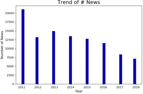
Factiva Real Estate News: A Self-Constructed Real Estate News Corpus In this research, I construct a real estate news corpus on my own, as there’s no existing prepared news corpus specific to real estate. I download and clean 102,402 news articles from a Financial News Database, Factiva. Those articles are all under the Factiva directory subject: real estate market and region: United States, and in English language. Their dates range from 2011-01-03 to 2018-12-31, including almost every single day in between. More news articles are available for the first few years, especially 2011, than recent ones (See Figure 4-1). This could be because there were a lot of hot discussions and focus on the real estate market after the financial crisis. For this research, I only focus on the headlines of these news articles, since headlines normally summarize the news content in a brief way, using generally simple and direct expressions.
Figure 4-1: The number of news in each year.
Figure 4-2 presents an example of the Factiva database. The screenshot was taken on Nov 8th 2018. As stated above, the results are filtered to show only the news in the real estate market subject related to the United States. Clearly, we can see that the news returned by Factiva covers most of the important information about
the real estate market at that time. Besides, a closer study on the headlines indicate that it’s reasonable for us to set the goal of extracting both the market event and the sentiment from the headlines.
Figure 4-2: An example of the Factiva database.
For each piece of news, I follow the open-sourced codes1 to extract relevant features.
Several variables are collected, including its headline, word count, publication time, author, and source name. Then we employ the following two criteria to clean the news data.
Cleaning criterion 1: word count ≤ 90% quantile
This is mainly because some news collected in the corpus may not be directly related to the real estate market. For example, a large amount of news titled the U.S. Eco-nomic Calendar are included in the corpus, which are just ecoEco-nomic reviews rather
1
than newly published events. Given the fact such economic reviews are often very lengthy, we remove all the news whose word count is less or equal than the 90% quantile, which is 2,071 words.
Cleaning criterion 2: the headline should appear only once.
This criterion mainly targets the duplicates of news. All of the news which appear several times are removed from the corpus, because such titles are likely to be the column name of a newspaper, instead of the summarized news content which records the real-time market events. Examples of removed headlines by these two critera in-clude: US Economic Data Calendar; Building Permits; News Highlights: Top Global Markets News of the Day, etc.
Finally, 79,627 news are selected from altogether 102,402 raw samples.
Figure 4-3: An example of the Factiva database.
Figure 4-3 shows the frequency distribution of the number of news published by each news source, where the y-axis is in log scale. As we can see, the majority of news in
the dataset are published by a source that only release only one or a few news, which guarantees that the news in our self-constructed corpus comes from a diverse range of sources.
Financial PhraseBank – a Financial News Corpus
Given that there is no corpus available with sentiment labels specific to real estate, I used a financial news corpus instead, the Financial PhraseBank (Malo et al., 2014). This dataset is a collection of 4,840 sentences from financial and economic news, which I expect to carry rich domain information, and to be predictive for the real estate market as well. Each sentence is manually annotated by 5-8 finance and economics ex-perts, with the sentiment label “positive”, “negative” or “neutral”. Sometimes different experts may have different interpretations on a sentence and give different sentiment labels. Therefore, four sub-datasets are provided with different level of agreements (see Table 4.1). Given that the sample size of this dataset is relatively small, I simply used all 4,840 samples provided.
Table 4.1: Sentiment distribution of sentences in Financial PhraseBank. Sub-datasets % Negative % Neutral % Positive Count Sentences with 100% agreement 13.4 61.4 25.2 2259 Sentences with >75% agreement 12.2 62.1 25.7 3448 Sentences with >66% agreement 12.2 60.1 27.7 4211 Sentences with >50% agreement 12.5 59.4 28.2 4840
ACE 2005
The Automatic Content Extraction (ACE) 2005 corpus is created and maintained by the Linguistic Data Consortium of the University of Pennsylvania, which contains human-labeled text documents from a variety of sources, such as newswire reports, weblogs, and discussion forums. In general, we have 14,766 sentences in the training data, among which 3,526 sentences contain at least one labeled event. The number of events contained in one sentence ranges from 1 to 7, with its distribution shown in
Table 4.2. In total, there are 4,704 event triggers. These triggers are further divided into 8 classes (see Table 4.3). We can see that there are significant imbalances in this dataset. More than 75 % (11240/13766) of the sentences contain no triggers; and the Conflict class contains over 13 times more triggers than the Business class. These imbalances cause additional challenges on our event detection task.
Table 4.2: Trigger statistics of ACE 2005 corpus.
# Events 0 1 2 3 4 5 6 7 # Sentences 11240 2625 688 166 33 12 1 1
Table 4.3: Class statistics of ACE 2005 corpus.
Class Business Conflict Contact Justice Life Movement Personnel Transaction # Triggers 110 1485 342 604 805 662 429 267
Below shows an example data entry of the ACE 2005 dataset. As we can see, each data entry contains a complete sentence, as well as its tokens, parsing, part-of-speech, etc. Our learning goal is the key ‘golden-event-mentions’, which records the labeled events contained in the sentence, triggers and arguments included.
{
"sentence": "He visited all his friends.",
"tokens": ["He", "visited", "all", "his", "friends", "."], "pos-tag": ["PRP", "VBD", "PDT", "PRP$", "NNS", "."], "golden-event-mentions": [ { "trigger": { "text": "visited", "start": 1, "end": 1 }, "arguments": [
{ "role": "Entity", "entity-type": "PER:Individual", "text": "He", "start": 0, "end": 0 }, { "role": "Entity", "entity-type": "PER:Group", "text": "all his friends", "start": 2, "end": 5 } ], "event_type": "Contact:Meet" } ], "golden-entity-mentions": [ { "text": "He", "entity-type": "PER:Individual", "start": 0, "end": 0 }, { "text": "his", "entity-type": "PER:Group", "start": 3, "end": 3
}, {
"text": "all his friends", "entity-type": "PER:Group", "start": 2,
"end": 5 }
],
"parse": "(ROOT\n (S\n (NP (PRP He))\n (VP (VBD visited)\n (NP (PDT all) (PRP$ his) (NNS friends)))\n (. .)))"
} ]
Corpus Preprocessing
The financial sentences in Financial PhraseBank, and the news headlines in my real estate corpus are both preprocessed by the following steps:
∙ Replace all special symbols in the string with blanks ∙ Convert all letters to their lower case
∙ Tokenization - convert sentences to words either by spliting the sentence by space, or by virture of the Tokenizer
∙ Lemmatization - reduce each word to its root by removing inflection
∙ Time Match - for the Factiva Real Estate News, we match the publication date of each news to the closet next working day, if the news is published during the weekends. This is because we are studying the market response to these news. Hence, we assume the effect of all news over the market closing will accumulate and be realized once the market is reopened.
4.1.2
Numerical Data
Numerical data are real-valued variables used in this research, most of which are economic variables.
REIT Price Time Series
REIT price index, a daily time series, is the final prediction goal in our regression problem. I download and clean the daily Wilshire REIT index from the Federal Reserve Economic Data2, for each trading day between 2011-01-03 to 2018-12-31, so that the news corpus could match the price data. Note that the Wilshire REIT index include both the price return and the total market return. The difference between the two is that the total market return counts in the dividend return, while the price return doesn’t. Since we study the REIT pricing model for both future investment or market monitoring, we use the total market return in this research.
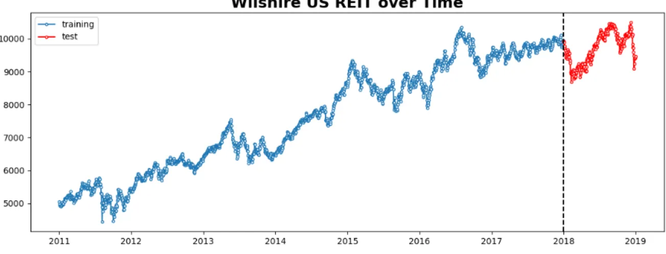
As we can see in Figure 4-4, the time series of REIT index is not stationary, as it has a clear increasing trend. However, we could still observe some small market falls from time to time, despite the fact that our targeted time period doesn’t include the 2008 financial crisis.
Figure 4-4: Trend of the REIT index (Wilshire US REIT).
As Figure 4-4 shows, we divide the entire time series into the training data and test
2
data. The training data includes all observations between 2011 and 2018, which I use to train my REIT pricing model. On the contrary, the test data is used to evaluate the model performance, by comparing the real price and the forecast price predicted by the trained model. The REIT index time series contain 2,090 observations in total, including 1,827 training data and 263 test data.
NAV Premium
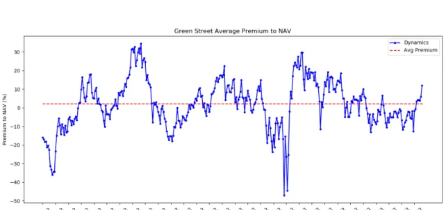
Since the REIT price is mainly backed up by its net asset value (NAV), we must include the NAV as an explanatory variable. In order to obtain an accurate measure of NAV, we scraped the monthly average premium to NAV published by the Green Street advisor3, and derive the NAV measurement based on the following equation. Figure 4-5 presents the scraped premium to NAV data between 1990-02 and 2019-02. The average monthly premium to NAV is 2.00% in this period.
NAV =
REIT index
1+premium to NAV (4.1)
Figure 4-5: The NAV premium.
3
Figure 4-6: The NAV premium betwen 2009 and 2018.
Figure 4-7: Comparing the trend of REIT index and NAV.
We match the Green Street premium to NAV to our target period, 2009-2018 (See Figure 4-6). During our targeted period, the average premium to NAV is 3.95%, which is almost twice as high as that of the entire period between 1990 and 2018. This might be a warning signal to the market, and also indicate there might be behavioral factors playing a role. Figure 4-7 compares the trend of the REIT index and the NAV that
we derive based on the Green Street premium to NAV. Clearly, NAV has the similar trend as the REIT index, indicating its significant role in REIT pricing.
4.1.3
Fama-French Factors
According to the asset pricing theory, the Fama French factors, including Rm-Rf (ex-cess return on the market portfolio), SMB (small minus big, i.e. size premium) and HML (high minus low, i.e. value premium), are also included to control the gen-eral market conditions. These factors are obtained from Professor French’s personal website4, and are in daily basis.
4.1.4
Growth Opportunities
According to the asset pricing theory, the expected growth rate is very important in determining the price of an asset, as it affects future cash flows in an exponential way. Higher expected growth corresponds higher cash inflow in the future, and hence higher current price.
𝑃𝑟𝑒𝑖𝑡 = 𝑥𝐹 𝐹 𝑂 𝑘𝑟𝑒𝑖𝑡− 𝑔𝑟𝑒𝑖𝑡 ≈ 𝑥(𝑁 𝑂𝐼 − 𝐼) 𝑘𝑟𝑒𝑖𝑡− 𝑔𝑟𝑒𝑖𝑡 (4.2) In the REIT valuation framework proposed by Clayton & MacKinnon (2002), 𝑔𝑟𝑒𝑖𝑡, the
expected constant growth rate of the REIT dividends, also plays a role. This suggests that we should include some measurements of REIT growth opportunities in our REIT pricing model. To this end, I collected every IPO (initial public offering), SEO (second equity offerings), and SDO (second debt offerings) case from the Nareit (The National Association of Real Estate Investment Trusts) website5. Fortunately, they provide the
precise date for each capital offering, so I can match them with the news and other economic variables. The capital offerings are summed by type (IPO/SEO/SDO) and by month, assuming that the expected growth rate keeps constant within one month. Although the precise date for each case is available, it may not be correct to use daily expected growth since people’s expectation on some asset class should be
4
http://mba.tuck.dartmouth.edu/pages/faculty/ken.french/data_library.html
5
relatively stable in a given period of time. To sum up this section, we’ve collected and generated four main numerical variables for the REIT pricing model, including (1) the daily REIT index; (2) the monthly premium to NAV and derived daily NAV; (3) the daily Farma-French factors; and (4) the monthly REIT capital offerings. All variables are merged together based on their timestamps.
4.2
Exploratory Analysis
In this section, we present some preliminary analyses on the REIT index. As men-tioned before, the non-stationarity of the REIT index series prevents us from further estimation. Therefore, I first conduct some stationarity check on the REIT index.
Taking the Difference
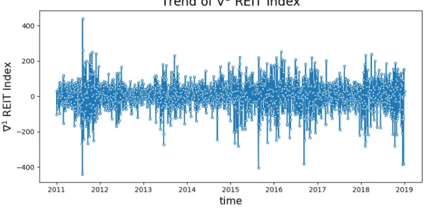
We first take the first and second-order difference and visualize them in Figure 4-8 and Figure 4-9. Clearly, both graphs show a pattern of zero mean and approximately constant variance, which suggests the series might become stationary after taking the difference. However, more rigorous analysis is needed.
Figure 4-9: The second order difference of REIT Index.
Suppose the time series is a collection of random variables 𝑋0, · · · , 𝑋𝑛 indexed in
time, a typical way to check the dependence between the random variables across time is to calculate the Autocorrelation (ACF) and Partial Autocorrelation (PACF). Based on the estimates, we could determine whether we should fit the series by a Autoregressive (AR) model, or a Moving Average (MA) model.
In an AR(p) model, we assume the time series is generated by
𝑋𝑡= 𝜑1𝑋𝑡−1+ 𝜑2𝑋𝑡−2+ · · · + 𝜑𝑝𝑋 𝑡−𝑝+ 𝑊𝑡 (4.3)
where 𝑊𝑡 is the white noise.
In a MA(q) model, we assume the time series is generated by
𝑋𝑡 = 𝑊𝑡+ 𝜃1𝑊𝑡−1+ 𝜃2𝑊𝑡−2+ · · · + 𝜃𝑞𝑊𝑡−𝑞 (4.4)
Combining the AR and MA model, we could also fit the series by using an ARMA(p,q) model, which is
𝑋𝑡= 𝜑1𝑋𝑡−1+ 𝜑2𝑋𝑡−2+ · · · + 𝜑𝑝𝑋𝑡−𝑝+ 𝑊𝑡
+ 𝜃1𝑊𝑡−1+ 𝜃2𝑊𝑡−2+ · · · + 𝜃𝑞𝑊𝑡−𝑞
Based on the temporal dependence pattern of the REIT index, we should choose a suitable model accordingly.
ACF
Marginal mean 𝜇𝑋(𝑡) = E[𝑋𝑡]
Autocovariance 𝛾𝑋(𝑠, 𝑡) = 𝑐𝑜𝑣(𝑋𝑠, 𝑋𝑡) = E[(𝑋𝑠− 𝜇(𝑠))(𝑋𝑡− 𝜇(𝑡))]
Autocorrelation (ACF) 𝜌𝑋(𝑠, 𝑡) =
𝛾𝑋(𝑠, 𝑡)
√︀𝛾𝑋(𝑠, 𝑠)𝛾𝑋(𝑡, 𝑡)
(4.6)
Clearly, the autocorrelation 𝜌𝑋(𝑠, 𝑡) measures the linear dependence of 𝑋𝑠 and 𝑋𝑡,
and should be between -1 and 1. For weak stationary series, the autocorrelation can be further simplified as 𝛾𝑋(𝑡, 𝑡 + ℎ) = 𝛾𝑋(0, ℎ) =: 𝛾𝑋(ℎ).
With enough observations, the sample mean and autocorrelation for stationary time series can be estimated as:
sample mean ^𝜇𝑋 = ¯𝑥 = 1 𝑛 𝑛 ∑︁ 𝑡=1 𝑥𝑡 sample autocovariance 𝛾𝑋(𝑠, 𝑡) = 1 𝑛 𝑛−|ℎ| ∑︁ 𝑡=1 (𝑥𝑡− ¯𝑥)(𝑥𝑡+|ℎ|− ¯𝑥), for − 𝑛 < ℎ < 𝑛
sample autocorrelation (ACF) ^𝜌𝑋(ℎ) = ^𝛾𝑋(ℎ)/^𝛾𝑋(0), for − 𝑛 < ℎ < 𝑛
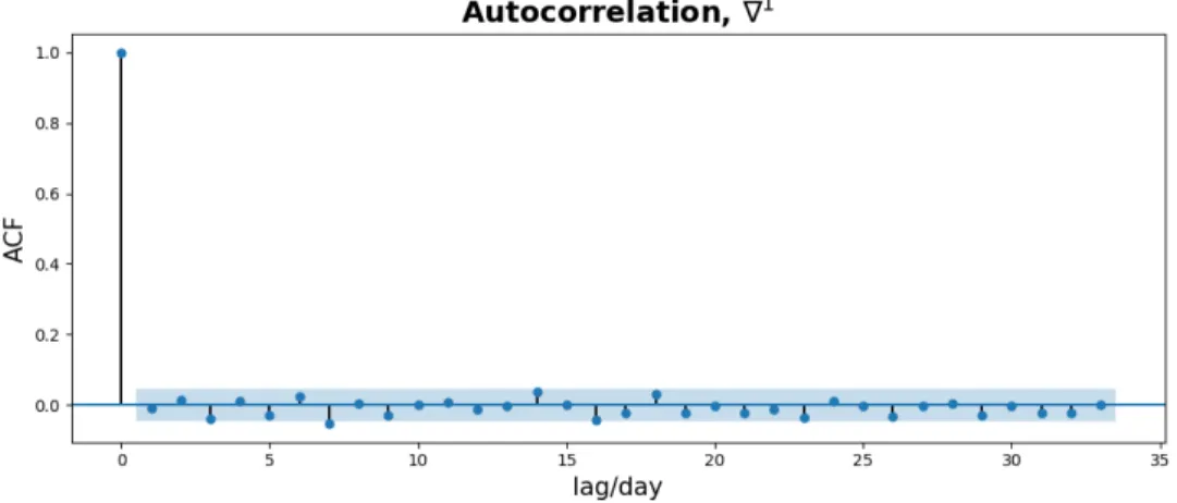
(4.7) Figure 4-10 and Figure 4-11 present the ACF estimates of the REIT index series after taking the first and second-order difference. As we can see, the ACF estimate is 0 for any ℎ (i.e. lag of days) for ∇1 REIT, which suggests that it could fit a white noise model. For ∇2 REIT, the ACF estimate becomes 0 when ℎ > 1, indicating that we
Figure 4-10: The ACF estimate of the first-order differenced REIT index..
Figure 4-11: The ACF estimate of the second-order differenced REIT index.
PACF
We also estimate the partial autocorrelation for the REIT index after taking the first and second order difference (see Figure 4-12 and Figure 4-13). The basic idea of PACF is the conditional autocorrelation, which measures the correlation between 𝑋𝑡
and 𝑋𝑡−ℎ conditioned on all variables in between. That is,
𝜑ℎℎ= 𝑐𝑜𝑟𝑟(𝑋𝑡− ^𝑋𝑡, 𝑋𝑡−ℎ− ^𝑋𝑡−ℎ) (4.8)
where ^𝑋𝑡 and ^𝑋𝑡−ℎ are the linearly fitted values of 𝑋𝑡 and 𝑋𝑡−ℎ on the subspace
𝑋𝑡−1, · · · , 𝑋𝑡−ℎ+1.
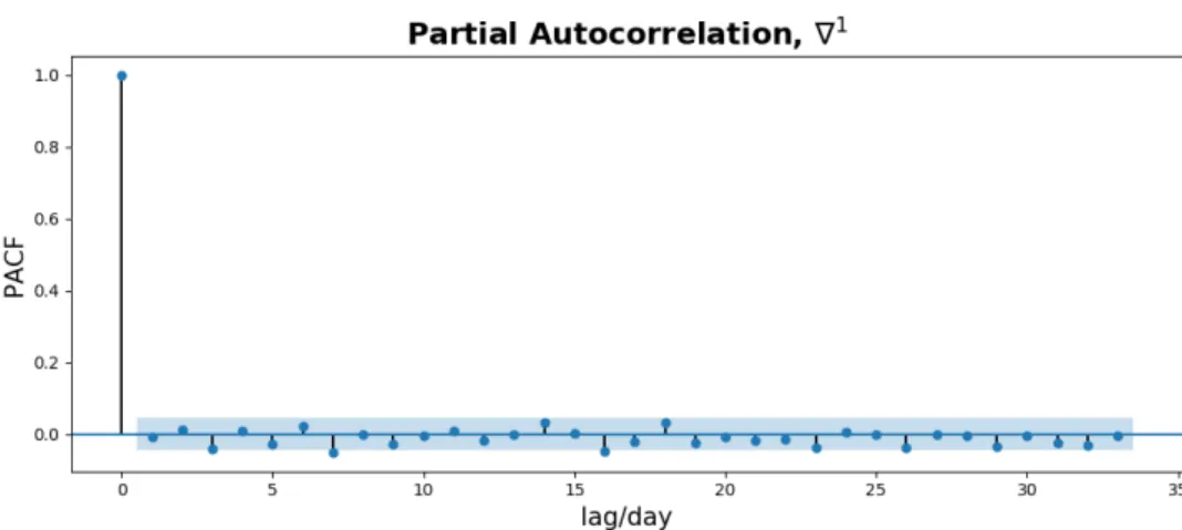
Figure 4-12: The PACF estimate of the first-order differenced REIT index.
Figure 4-13: The PACF estimate of the second-order differenced REIT index. Again, the PACF estimate suggests that the REIT index could be fit by a white noise model after taking the first difference. Besides, since the PACF decays and tails off for the second-order differenced REIT index, a MA model should be chosen.
4.3
REIT Pricing Models
This section discusses the methods to fit and predict the U.S. REIT index between 2011 and 2018, with a bunch of numerical and textual information. As explained above, numerical information include the derived NAV, the Fama-French factors, and
the capital offerings. To compensate for the low-frequency of market fundamentals, real-time market events and sentiment, as textual information, will be extracted and processed by NLP techniques.
I will first conduct the traditional time series analysis by estimating the ARIMA and Vector Autoregressive (VAR) models, and then compare it with the deep learning methods. The advantage of traditional econometric models lies in its interpretability, given that the model goes straightforward without any hidden layers. Besides, con-sidering the possible reverse causality problem between sentiment and price, it can also check how sentiment and events are backed up (sentiment/events ∼ price), in addition to price prediction (price ∼ sentiment/events). In contrast, deep learning model with word and event embeddings might be good for predictions, but it’s hard to interpret since the word/event vectors don’t have any economic meanings. However, traditional time series analysis suffers from great limitations, in that it lacks predic-tion accuracy since we can’t generate event-related variables which carry as much information as word and event embeddings. This implies that a trade-off between interpretability and prediction accuracy is inevitable.
4.3.1
Time Series Analysis
Autoregressive Integrated Moving Average (ARIMA)
ARIMA is an extension of the aforementioned ARMA models, where the value of the time series at a time step is regressed on both the AR(p) and MA(q) variables. However, different from ARMA, ARIMA does not fit the original value, but the difference of some order. The order of order of difference is a parameter in the ARIMA(p,d,q) model. In this research, we will estimate the following ARIMA model,
∇𝑝𝑅𝐸𝐼𝑇𝑡= 𝜑1∇𝑝𝑅𝐸𝐼𝑇𝑡−1+ 𝜑2∇𝑝𝑅𝐸𝐼𝑇𝑡−2+ · · · + 𝜑𝑝∇𝑝𝑅𝐸𝐼𝑇𝑡−𝑝+ 𝑊𝑡
+ 𝜃1𝑊𝑡−1+ 𝜃2𝑊𝑡−2+ · · · + 𝜃𝑞𝑊𝑡−𝑞 + 𝑒𝑥𝑜𝑔
(4.9)
where exog stands for the exogenous variables, and the choice of p, d, q are determined by the Akaike information criterion (AIC).
Vector Autoregressive (VAR)
As the vector version of AR model, VAR also regresses time series variables on its previous values. The difference lies in that the VAR regresses on the previous values of all variables in the vector.
In this research, I regress the change in REIT index (∇𝑅𝐸𝐼𝑇 , first order difference) on previous NAV, Fama-French factors, capital offerings and market sentiment. Specif-ically, we estimate the following model, where the first equation shows the effect of lagged sentiments on the change in the REIT index at current time, while the second equation reveals the impact of lagged change in REIT index on current sentiment.
∇𝑅𝐸𝐼𝑇𝑡= 𝑐1+ 𝐴1,1∇𝑅𝐸𝐼𝑇𝑡−1+ ... + 𝐴1,𝑝∇𝑅𝐸𝐼𝑇𝑡−𝑝
+ 𝐴2,1𝑠𝑒𝑛𝑡𝑖𝑚𝑒𝑛𝑡𝑡−1+ ... + 𝐴2,𝑝𝑠𝑒𝑛𝑡𝑖𝑚𝑒𝑛𝑡𝑡−𝑝+ · · ·
𝑠𝑒𝑛𝑡𝑖𝑚𝑒𝑛𝑡𝑡= 𝑐2+ 𝐵1,1∇𝑅𝐸𝐼𝑇𝑡−1+ ... + 𝐵1,𝑝∇𝑅𝐸𝐼𝑇𝑡−𝑝
+ 𝐵2,1𝑠𝑒𝑛𝑡𝑖𝑚𝑒𝑛𝑡𝑡−1+ ... + 𝐵2,𝑝𝑠𝑒𝑛𝑡𝑖𝑚𝑒𝑛𝑡𝑡−𝑝+ · · ·
(4.10)
One greatest advantage of the VAR model is that it enables the Granger causality test, which could reveal the causal relationship between sentiment and price change based on the statistics.
4.3.2
Big Picture: Deep Learning Task - Incorporating both
Textual and Numerical Information
In comparison with the traditional ARIMA and VAR methods, we will use the deep learning architecture in Figure 4-14 for the REIT pricing task, which is revised from Akita et al. (2016).
As discussed before, the deep learning model will take both textual and numerical datasets as the input. The raw numerical data will be the economic variables we collect and introduce in the previous sections, while the raw textual data will be the headlines from our self-constructed corpus.
For predicting the REIT index change at each time 𝑡, i.e. 𝑅𝐸𝐼𝑇𝑡 − 𝑅𝐸𝐼𝑇𝑡−1, we