MITLibraries
Document Services
Room 14-0551 77 Massachusetts Avenue Cambridge, MA 02139 Ph: 617.253.5668 Fax: 617.253.1690 Email: [email protected] http://iibraries.mit.edu/docsDISCLAIMER OF QUALITY
Due to the condition of the original material, there are unavoidable
flaws in this reproduction. We have made every effort possible to
provide you with the best copy available. If you are dissatisfied with
this product and find it unusable, please contact Document Services as
soon as possible.
Thank you.
Due to the poor quality of the original document, there is
some spotting or background shading in this document.
MASSACHUSETTS INSTITUTE OF TECHNOLOGY DEPARTMENT OF NUCLEAR ENGINEERING
Cambridge, Massachusetts
DESIGN OF A COLD NEUTRON SOURCE FOR THE MIT REACTOR
by
R. C. Sanders, D. D. Lanning, T. J. Thompson
May, 1970
ABSTRACT
A new design for the MIT reactor thermal column has been developed to increase the thermal neutron flux in that region. By removing graphite from the thermal column and creating a cavity with graphite walls, it is possible to in-crease the thermal neutron flux by a factor of about 30.
The location of a scattering material, such as a cold neutron moderator, in the cavity does not greatly reduce this increase in neutron flux, but does cause an asymmetry in the flux in-cident on the scatterer. The flux incident on the source side of the scatterer is approximately 60% higher than the flux in-cident on the back side.
A cold neutron cryostat has been designed, built, and tested in the present MIT reactor thermal column. The
cryostat consists of a 12 inch diameter aluminum sphere con-taining D 0 ice cooled by cold gaseous helium in aluminum
coils. Te sphere is surrounded by an aluminum vacuum jacket
to form the cryostat. Initial testing indicates that the cryostat is effective in increasing the number of long wave-length neutrons. For a cold D 20 moderator temperature of a
-40C the measured increase in neutrons of 5 a wavelength is about a factor of 1.8. From this experimental result it is o
estimated that there will be a factor of about 50 gain in 5 A neutrons for a moderator temperature of 201K.
The expected neutron spectrum in the cold moderator has also been calculated theoretically. The theory predicts the observed increases in cold ngutron intensities; however, it over estimates the gain in 5
A
neutrons by a'bout 25%. This difference falls within the uncertainty in the value for the effective mass of the D 20 ice..BLANK PAGE
ACKNOWLEDGMENTS
The author thanks Dr. Theos. J. Thompson for his assistance and guidance as the initial supervisor of this work. He ex-presses his appreciation to Dr. David D. Lanning who assumed the position of thesis supervisor when Dr. Thompson undertook the role of AEC Commissioner in 1969. He also thanks Dr. N. Thomas Olson, the thesis reader, for his helpful suggestions, especially in the writing of the manuscript.
The assistance of Dr. Yoshiguti Hukai and Mr. Ronald J. Chin in carrying out the experimental work is greatly ap-preciated. Dr. Franklyn M. Clikeman and Mr. David A. Gwinn
are thanked for the assistance they provided in setting up the electronics of the neutron detection system.
The author would like to thank the MIT Reactor Staff, the Reactor Machine Shop, the Reactor Electronics Shop, and the Radiation Protection Office for their assistance and sug-gestions.
The typing was done by Mrs. Carol Lindop, and the drawings by Mr. Leonard Andexler. Their assistance is appreciated.
Miss Roberta Dailey is also thanked for her assistance in pre-paring the final manuscript.
The computations for this thesis have been done in part at the MIT Information Processing Center on the IBM 360/65.
The author was supported in part by an Atomic Energy Commission Fellowship in Nuclear Science and Engineering, and
by a National Science Foundation Graduate Fellowship.
This project has been supported by a Sloan Pure Physics Research Grant.
TABLE OF CONTENTS Page Title Page Abstract Acknowledgments Table of Contents List of Figures List of Tables Chapter 1 Chapter 2
Chapter 3
Chapter 4
Chapter 5
IntroductionHohlraum Flux Calculations 2.1. Method
2.2. Rectangular Cavities
2.3. Dis.cussion of Assumptions Test of Model
3.1. Comparison with Experiment 3.2. Lead Shutters
Optimization of Thermal Column 4.1. Empty Cavity
4.2. Comparison with Solid Thermal Column 4.3. Effect of Coolant Pipes
4.4. Plane Object in Cavity 4.5. Effect on Lattice Facility 4.6. Summary
Cold Neutron Cryostat
5.1. Description of Cryostat
6
1
6
12
13
17
17
22
25
28
28
32
39
39
43
45
48
53
56
58
58
Chapter 6
Chapter 7
Chapter 8
Appendix A
Appendix B
Appendix C
Appendix D
5.2.
Cryostat Heating
5.3.
Helium Pressure Drop
Cryostat Testing
6.1. Out of Pile Testing
6.2. In Pile Testing
6.3. Flux Measurements
Flux Calculations in Cold Moderator
7.1. Method of Calculation
7.2. Results
7.3. Comparison with Experiment
Conclusions and Recommendations for
Future Work
8.1. Conclusions
8.2. Recommendations for Future Work
Calculation of View Factors
A.l. View Factors for Parallel Planes
A.2. View Factors for Perpendicular Planes
A.3. Computer Program for Calculating View
Factors
Computer Programs for Calculating Fluxes in
a Cavity
B.l. HOLCAV
B.2. TARGET
Lead Shutter Shielding Effects
Cryostat-Heat Load Calculations
D.l. Thermal Column Flux Measurements
D.2. Core Gamma Heating
D.3. Graphite Gamma Heating
7
Page
67
71
74
74
81
86
96
96
98
111
115
115
117
119
119
123
127
134
134
135
170
187
187
189
193
Appendix E
D.4. Fast Neutron Heating
D.5. Cryostat Gamma Heating
D.6. Radiant Heat Transfer
D.7. Free Molecular Conduction
D.8. Thermal Conduction
Helium Pressure Drop Calculations
E.l.
Supply and Return Lines
E.2. Cooling Coils
References8
197
199
202
205
208
203
209
211
V,
LIST OF FIGURES Figure 2.1. 2.2.3.1.
3.2.
3.3.
3.4.
3.5.
3.6.
4.1.
4.2.4.3.
4.4.
4.5.
5.1.
5.2.
5.3.
5.4.
5.5.
5.6.
5.7.
6.1.
6.2.
9
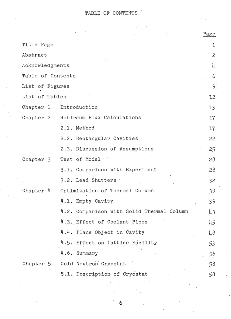
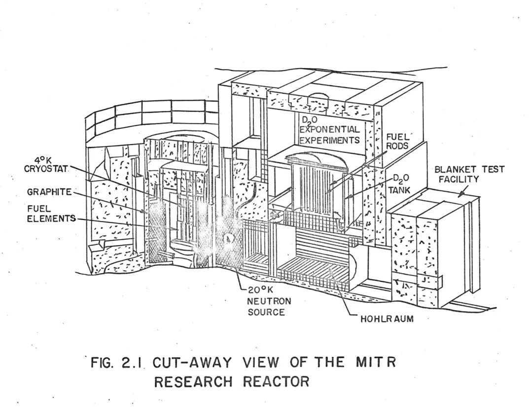
PageCut-Away View of the MIT Research Reactor
Rectangular Cavity Showing.Relationship between Faces and Coordinates
Hohlraum Showing Relationship between the Faces
Hohlraum, Face 1 Fluxes on Pedestal
Lead Shutter, No Lining
Lead Shutter, 12 inch Lining
Flux Across Centerline of Thermal, Column Face
Modified Thermal Column Flux on Face 2
Location of Coolant Pipes Plane Object in Cavity
Flux on Surface of Plane Object Cold Neutron Cryostat
Upper Shield Block Vacuum Region
Cold Moderator
Beryllium Filter Assembly Helium Supply System
Temperature Distribution in D 0 Ice
2
Freezing Test Water Temperature18
23
29
30
31
34
35
37
40
42
46
49.
52
59
60
61
63
65
66
72
75
77
Figure
Page
6.3.
Sphere Deflection
79
6.4.
Water Temperature
82
6.5.
Spectrum Measuring Equipment
87
6.6.
Neutron Spectrum in Graphite Thermal
Column
88
6.7.
Neutron Spectrum in Warm D
20
90
6.8.
Neutron Spectrum in D
20 Ice at 3
0C
92
6.9.
Neutron Spectrum in D
20 Ice at -40*C
93
6.10.
Measured Neutron Spectra
94
7.1.
Model of Cold Moderator
97
7.2.
Neutron Spectrum in Graphite
100
0
7.3.
Cold Neutron (X>3.96 A) Gain
101
7.4.
Cold Neutron (X>3.96 A) Gain
103
0
7.5.
Cold Neutron (X>3.96 A) Gain
105
0
7.6.
Cold Neutron (X>3.96 A) Gain
108
7.7.
Neutron Spectrum in Cold Moderator
107
7.8.
Cold Neutron Gain
108
7.9.
Cold Neutron Gain
110
7.10.
Neutron Wavelength Distributions
112
7.11.
Neutron Spectrum in Warm Graphite
114
A.l.
Subareas on Parallel Planes
12~0
A.2.
Subareas on Perpendicular Planes
124
C.l.
Relative Po-itions of Lattice Room,
Hohlraum, and Shutter
171
C.2.
Hohlraum Slow Neutrons
180
Figure
Page
C.t4.
Hohlraum Gammas
182
C.5.
Lattice Room Slow Neutrons
183
0.6.
Lattice Room Fast Neutrons
184
C.7.
Lattice Room Gammas
1-85
D.l.
Model for Graphite Gamma Heating
194
LIST OF TABLES Table
4.1.
4.2.
5.1.
5.2.
6.1.
C.l.
C.2.
C.3.
C.
4.
C.5.
D.l. D.2.D.3.
D.
4.
D.5.
D.6.
S
D.-7.
D.8.
D.9.
D.
10.
Length of Subarea Edge Measured Cadmium Ratios
Cryostat Heat Load Helium Pressure Drop
Empty Cryostat Temperatures, OF
Shield Combinations Dose Rates in Hohlraum Dose Rates in Hohlraum Dose Rates in Lattice Room Dose Rates in Lattice Room Thermal Column Flux Data
Group Constants for Core Gamma Heating Core Gamma Heat Load
Constants for Graphite Gamma Heating. Graphite Ga1ima Heat Load
Fast Neutron Heat Load
Group Constants for Aluminum Gamma Heating
Cryostat Gamma Heat Load Radiant Heat Load
Free Molecular Conduction Heat Load
12
Page
41
55
68
73
84
170
173
175
176
178
188
192
193.
196
197
199
201
202
203
205
Chapter 1 Introduction
Cold neutrons are defined as those neutrons having energies 0
less than 0.005 ev or wave-lengths longer than about 4 A. At these wave-lengths cold neutrons become important tools in material science because their wavelength is on the order of
lattice spacings in solids.
For several years X-rays have been used for studying
materials. Cold neutrons can now be used to extend the range of these studies. First, X-rays interact with atoms while neutrons interact with nuclei. Thus, cold neutrons can give more detailed information about the lattice; for example, the magnetic dipole
moments* of the atoms making up the lattice.
Secondly, because of their much shorter interaction time with the lattice, X-ray see the static position while cold neu-trons see position as a function of time, and thus more infor-mation is obtained abouu the thermal motions of the lattice. The vibrational period of a lattice is on the order of 10 14
seconds compared with a traverse time of 10- 18seconds for an X-ray, and 3 X 10 seconds for a 0.005 ev neutron.
The energy of the X-ray scattered from the atom is inde-pendent of the thermal motions of the atom; whereas, a scattered neutron can either gain or loose energy, depending on the
thermal motion of the scattering nucleus. Therefore, the cold neutron can give information about the type and energy of the thermal motion of the atom in the lattice (26).'
Although cold neutrons are effective tools, their use has
been limited because of the low intensity of beams usually available from thermal reactors. The thermal neutron spectrum of such a reactor is very nearly a maxwellian distribution at the temperature of the moderator which is typically above
0
3000K. At this temperature the flux of 4 A neutrons is less 0
than 1/16 the maximum flux, while the flux of 8 A neutrons is less than 1/14 the 4 A flux (27).
One method of increasing the cold neutron fraction of the neutron spectrum is to extract the beam from near the reactor core where t-he thermal flux is the highest and eliminate that
0
part of the spectrum with wavelengths shorter than 4 A by using a beryllium filter; however, in this case the cold neutron beam has a high probability of being hidden in the fast neutron and gamma ray background. With this in-mind the obvious method of obtaining a high intensity cold neutron beam appears to be to increase the cold neutron fraction of the thermal spectrum through the use of a cold moderator located where the fast neutron and gamma ray fluxes are minimal.
Ideally the cold moderator shifts the thermal neutron spectrum from that characteristic of the reactor temperature (on the order of 300'K) to a spectrum characteristic of the temperature of the cold moderator (1000K or less). This will increase the relative number of low energy neutrons. To do this it is necessary for the cold moderator to have a large
slowing down power and a low absorption cross section.
Hydrogenous materials have'high slowing down powers;
however, because of the high hydrogen absorption cross section that increases with decreasing neutron energy, a large fraction
of the cold neutrons are absorbed in the moderation and the maximum possible gain in cold neutrons is not realized. On the other hand, non-hydrogenous materials, such as deuterium oxide, beryllium, and graphite, with low absorption cross
sections; have relatively low slowing down powers and therefore large volumes are needed to obtain high cold neutron gains. Consequently a large cooling capacity is needed to maintain the moderator at a low temperature.
Another disadvantage of hydrogenous materials is their de-composition in a high radiation field. This presents the possi-bility of producing hydrogen gas in sufficient quantities to
form an explosive mixture with oxygen upon warming up the
moderator. On the other hand, heavy water is less susceptible to radiation damage (28).
To date several cold neutron sources have been located in various reactors (27, 29, 30, 31). In general these have been located in beam tubes of reactors and have been limited in size to a few hundred cubic centimeters. Consequently these cold neutron sources have not been efficient in producing high cold neutron gains; however, they have provided valuable information
about cold moderating materials.
In 1968, installation of a helium liquifying plant was initiated at the MIT reactor to provide coolant for an incore cryostat to be used to study radiation damage in materials. The plant is expected to deliver about 100 liters of liquid helium
per hour to the incore cryostat. The discharge from the incore
between 10 and 20 degrees Kelvin. With this large cooling capacity available, it was decided to locate a cold neutron
source in the thermal column of the reactor. 'This location has been selected for the following reasons.
First, with the large cooling capacity available, it is desirable to take advantage of a large volume of non-hydrogenous cold moderator. The thermal column provides the necessary space for such a moderator.
Second, with a large volume moderator the induced heating due to gamma rays and fast neutrons is appreciable. Consequently one would like to locate the cold moderator as far as possible from the reactor core, but still in a high thermal neutron flux. By removing graphite from the thermal column it is possible to create a cavity around the cold neutron source. Such a cavity allows neutrons to stream rapidly down the thermal column with a minimum amount of leakage out through the sides; thus, en-hancing the thermal flux available to the cold moderator.
The purpose of this work is twofold. First, Chapters 2 through 4 discuss the optimization of the thermal column. The effect of a cavity on the thermal flux in the thermal column
is investigated.. A detailed analysis is carried out to determine the optimum cavity size for the maximum thermal neutron flux.
Second, Chapters 5 through 7 discuss the design, con-struction, and testing of 15 liter cold neutron source which is located in the present thermal column, and is to be used to gain information about. and operating experience with a large volume cold neutron source. Also presented are calculations of the expected neutron spectrum in the- cold moderator.
Chapter 2
Hohlraum Flux Calculations
2.1. Method
A calculational model used for optimizing the thermal neu-tron flux in the thermal column is derived in this section. The thermal column is located between the reactor core and the heavy water lattice facility, as shown in figure 2.1. To enhance the
thermal flux in the thermal column, it is proposed to remove graphite from the thermal column; thus, creating a cavity or hohlraum with graphite walls. The method used to calculate the effect of such a cavity on the thermal flux in the thermal column i$ the same as that used by John Madell (2) in the de-sign of the hohlraum below the heavy water lattice facility
(figure 2.1).
Consider a cavity surrounded by reflecting walls, with .a
source of neutrons on one of the surfaces. Sinc- the cavity is filled with air, it will be assumed that the neutrons have an infinite mean free path in the cavity, and consequently suffer collisions only at the walls.
Let dA(r) be a differential area located at r on one of 2
the surfaces, and G(r) be the number of neutrons/cm sec in-cident on dA(r). Then G(r) dA(r) is the number of neutrons/ sec incident on dA(r).
Let S(r') be the number of neutron/cm 2.sec emitted.by the
source at r',.and K (r,r') be the probability that a neutron emitted at r'reaches r. Then the number of neutrons/sec emitted
HOHLR AUM
FIG. 2.1. CUT-AWAY
RESEARCH
VIEW OF THE MIT
R
REACTOR
I-J cxD
by the source at r' and reaching r is given by
f
S(r')K (rr')dA(r')' (2.1)Source r'
Let K2(r,r') be the probability that a neutron incident on the surface at r' be scattered back into the cavity and reaches r. Then the number of neutrons/sec reaching'r due to scatters at r' is given by
fG(r')K2(r,rl)dA(r'). (2.2)
All r'
Applyin'g a steady-state.neutron balance results in
G(r)dA(r) =
f
G(r')K 2(r,r')dA(rl)+f S(r')K 1 (r,rl)dA(rl).All r' Source r' (2.3)
The above equation is exact; however, it cannot be solved because of the unknown Kernals, K2 (r, r') and K1 (r,r'). Before
proceding, it will therefore be necessary to make some simpli-fying assumptions. These assumptions are discussed in a latter section of this chapter.
Since K2(r,r') is the probability that a neutron incident on the surface at r' is scattered back into the cavity and reaches r, it may be considered as the product of two proba-bilities. First is the probability that a neutron incident on the surface at r' be scattered back into the cavity at r'. In diffusion theory one defines the albedo as the ratio of the num-ber of neutrons/cm 2.sec leaving the surface to the number of neutrons/cm 2.sec entering the surface. This is the probability that neutrons entering the surface will be scattered back out; however it is an average effect over the entire surface and does
not take into account the fact that a neutron may enter the
sur-fac-e at one point and leave at another. The first assumption
then will be that the scattering (reflection) is a surface
effect and the albedo can be defined at a point.
Second is the probability that a neutron emitted at r'
reaches r. If it is assumed that the scattered neutrons and
the source neutrons are emitted from the surface according to
Lambert's Law; that is, the probability that a neutron leaves
the surface in solid angle dw at an angle
$'
with respect to the
normal to the surface is given by (1),
cos
$
dw
(2.4)
then equation (2.3) becomes,
G(r)dA(r)
=f
G(r')B(r')K (r,rT)dA(r)
+
f
S(r')K (r,r')dA(r')
All r
Source r'
(2.5)
where B(r') = albedo at r'
K 1(r,r') = co $dA(r) (2.6)
r-r
J
=distEnce from r to rl
= angle between the normal to
dA(r) and
(r-r')
cos$ rr' = Solid angle subtended by dA(r) at r'.
Using this, equation 2.4 becomes
G(r)dA(r)
=f
G(r')B(rt)[cos'cos$]dA(r)dA(r)
- Tr-j' 1.All r'
(2.7)
+f S(r')[2dA(r)dA(r ).
Source r'
20
Integrating over A(r.)
=A gives,
/G(r.)dA(r ) =f / G(r')B(r')[~"1o -1- ]dA(r)dA(r')
A-
A All r'
(2.8)
+
f f
S(r')[co
rS]dA(r)dA(r')
A-Source r'
In principle this equation can be solved for G(r) once
G(rl), B(r), and S(r') are specified.
In general these are not
known; powever the integration over r' can be performed if it
is assumed that the surfaces can be broken up into n small
sub-areas over which these quantities remain constant. The
inte-grations can then be carried out over each subarea and the
re-sults summed to give the total integral over r'.
It will also
be assumed that A is small enough that- G(r.) remains constant
over this area. Then the equation (2.8) becomes
all surfaces
G.A
=
E{G B fdA(r )f[coWcos ]dA(rn
1 n n IT- Lrri -n 12-al+EgouA r )/[c]Arkcos
(2.9)
.k
T-i k
IA(Lk)}'
A
Ak
Where G.= Average current incident on A
Gn
=
Average current incident on A.
n
n
Bn = Average albedo for An Sk = Average source for Ak But,
fdA(r )f[
r
]dA(rn
A Fni
(2.10)
A.
A
1 n
where Fni is the view factor from A to A.
Thus, equation
(2.9) becomes
all surfaces
all source
G.A. =
Z
G B A F n n n nl . + E S A Fk.kki(
(2.11)Equation (2.11) can be -written for each of the n subareas,
resulting in n equations and-n unknowns (n G.
's).
1
Once the currents are known, it is possible to determine
the flux on each of the subareas.
Since the flux is the
popu-lation of neutrons at the point of interest, it may be
con-sidered as the sum of the incident current and reflected current
from the subarea, or
Ph. = G. + RG. (2.12)
1 1 1
where Ph. is' the flux and RG. is the reflected current.
Rewriting gives
Ph. = G.[1 + B.] (2.13)
RG
t
where B.
i is
the albedo.
G.
2.2 Rectangular Cavities
Equation (2.11) is general for any geometry; however, only
in the special case of rectangular geometry can the view
fac-tors be found analytically. Since any modification to the
thermal column can be done most easily in rectangular geometry,
the advantage of this simplifying case will be taken in doing
the optimization calculations.
Consider a rectangular cavity as shown in figure 2.2, with
a source of neutrons incident on Face 1. The J's and K'.s are
coordinates describing the position of a subarea on a particular
RECTANGULAR CAVITY SHOWING
RELATIONSHIP BETWEEN FACES
AND COORDINATES
23
face; for example (Jl, Kl) means that the lower- left hand corner of a subarea on face 1 is at the position (Jl, Kl) and that it extends from Jl to Jl +L and from Kl to Kl +L Where L is the length of the side of the subarea. 'Also, take the subareas on all the faces to be the same size, so that the areas in equation 2.11 cancel out. Then, using computer program notation, equation 2.11 can be written for each of the faces as
HN WN GI(JI,KI) = E GN(JN,KN)BN(JN,KN)F(L1,L2,L3) KN JN Hl Wl + E E S(Jl,Kl)F(Ll,L2,L3) Kl Jl where N =1 to 6, except I HN = maximum value of KN WN = maximum value of JN F = view factor
Ll, L2, L3 = coordinates describing the relative positions of subareas.
For the view factor from a subarea on plane m to a subarea on a parallel plane-, n:
Ll = 1 +
IJm-JnI
L2 = 1 +IKm-Kni
L3 = Distance between planes.
For the view factor from a subarea on plane m to a subarea on a perpendicular plane, n:
Ll = distance from line of intersection of plands to subarea on m
L2 = distance of separation of the two subareas along the line of intersection
L3
=distance from line of intersection of the planes
to subarea on n.
Note that the equation for any face does not contain a term
which is the sum over that face (e.g. face 1 does not contain a
sum over the source).
This is due to the fact that the
sub-areas on a given face cannot see each other (i.e., the view
factors are zero).
The solution to equation 2.14 is obtained by an iteration
technique carried out on a digital computer. That is, initial
values for the G's are given and used to calculate new values
for the G's.
The initial values are then replaced by the new
values and again new values are calculated. This process is
continued until the G's converge (i.e., the calculated values
a-gree with the ones used to calculate them).
A description of the
computer program (HOLCAV) used to solve equation 2.14 is given
.in appendix B.
To solve equation 2.14 it is necessary to know the source
distribution, the albedes, and the view factors. The source
dis-tribution used for optimizing the thermal column is discussed in
-
Chapter
3.
A derivation of the view factors and a description
of the computer programs used to evaluate them are given in
appendix A. The albedos were determined by John Madell with a
Monte Carlo calculation and are taken from his thesis.
2.3. Discussion of Assumptions
mean free path in the cavity. For dry. air the mean free path for 2200 m/sec neutrons is 1811.cm. The measured- temperature in
the thermal column is about 700C (appendix D). At this tem-perature the saturation pressure of water is 234 mm Hg and the mean free path is 362 cm. A characteristic dimension for the proposed cavity is about 127 cm; therefore, the assumption of an
infinite mean free path is valid.
The second assumption is that the albedo can be defined at a point. Since equation 2.11 is for small subareas, this re-quirement ca-n be relaxed somewhat, in that now the albedo must be defined for a small area rather than for a point. This is the same as assuming that all the neutrons that return to
th th
the cavity from the i subarea were also incident on the i
subarea. That is, neutrons do not enter the wall through one subarea, scatter within the wall, and come out through a differ-ent subarea. Madell investigated this problem by means of a Monte Carlo calculation, and found that his albedos were acc.u-rate to about one percent provided the average caurrent over a subarea was within 10 percent of the currents incident on ad-jacent subareas. Except for the corners of the cavity, this condition is usually satisfied.
The third assumption is that the neutrons emerging from a surface do so according to Lambert's Law, that is the pro-bability of being emitted in solid angle dw at an angle $ with the normal to the surface is
cos4d T
Pigford et al
(3) have found that the actual
distribu-tion of neutrons being emitted from a-graphite surface is a
Placzek distribution (4), in which the neutrons emerge
pre-ferentially in the forward direction. This distribution is the
one that should be used in calculating the view factors;
however, its complicated form does not permit one to obtain
analytical expressions for the view factors. Madell found
that correcting to a Placzek distribution increased the
cal-culated fluxes by one or two percent. For this reason the
correction has not been applied in this work. This is also
justified by the excellent agreement between calculated and
measured fluxes (Chapter 3).
Chapter 3
Test of Model
3.1.
Comparison with Experiment
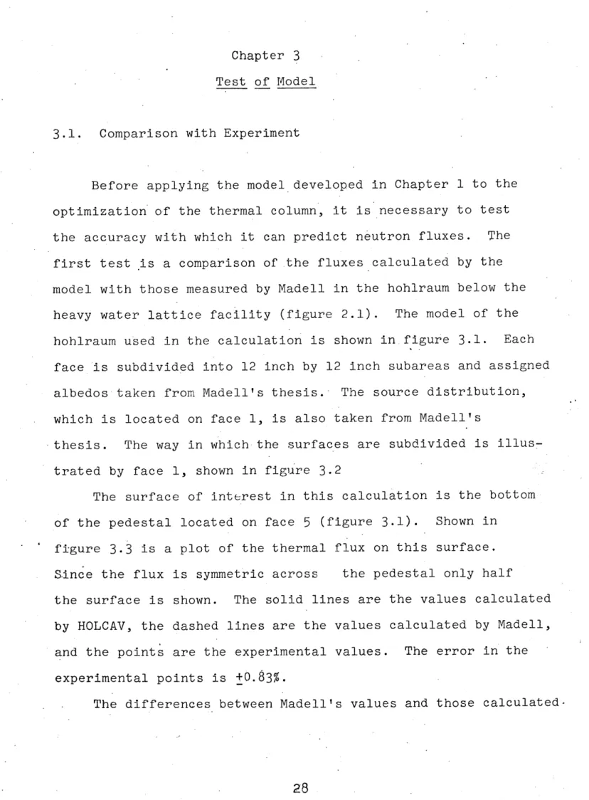
Before applying the model developed in Chapter 1 to the
optimization of the thermal column, it is necessary to test
the accuracy with which it can predict neutron fluxes.
The
first test .is a comparison of .the fluxes calculated by the
model with those measured by Madell in the hohlraum below the
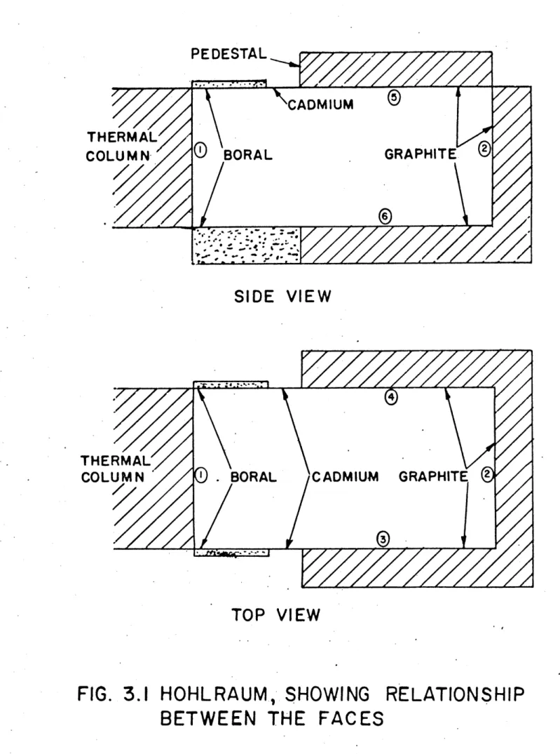
heavy water lattice facility (figure 2.1).
The model of the
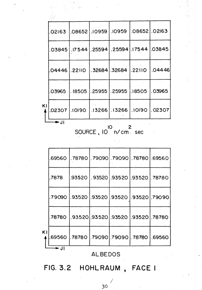
hohlraum used in the calculation is shown in figure 3.1. Each
face is subdivided into 12 inch by 12 inch subareas and assigned
albedos taken from Madell's thesis.- The source distribution,
which is located on face 1, is also taken from Madell's
*thesis. The way in which the surfaces are subdivided is
illus-trated by face 1, shown in figure 3.2
The surface of interest in this calculation is the bottom
of the pedestal located on face
5
(figure 3.1).
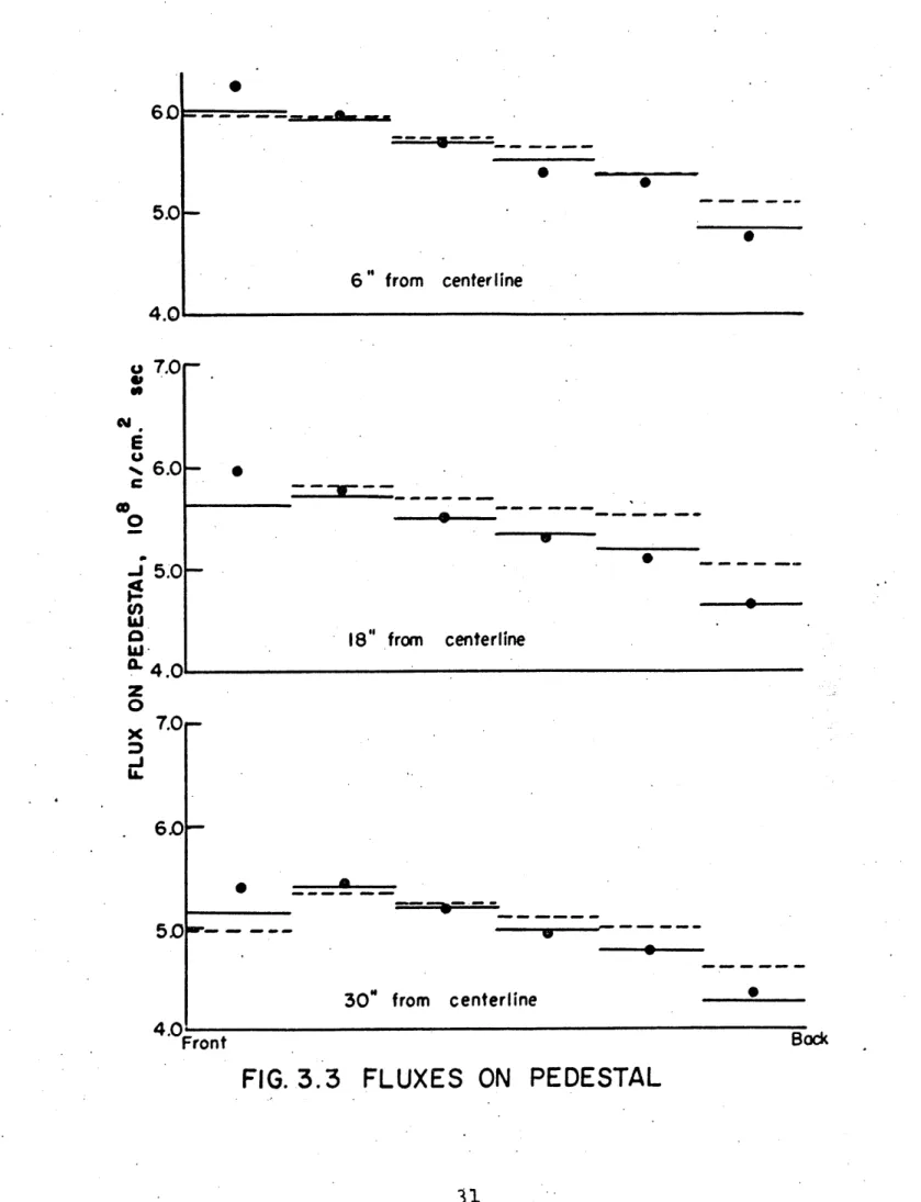
Shown in
figure 3.3 is a plot of the thermal flux on this surface.
S-ince the flux is symmetric across
the pedestal only half
the surface is shown. The solid lines are the values calculated
by HOLCAV, the dashed lines are the values calculated by Madell,
and the points are the experimental values. The error in the
experimental points is +0.83%.
The differences between Madell's values and those
29
PEDESTAL
THERMAL
COLUMN
0
BORAL
GRAPHITE
SIDE VIEW
COLUMN
.BORAL
CADMIUM
GRAPHITE
TOP VIEW
FIG. 3.1 HOHLRAUM, SHOWING RELATIONSHIP
BETWEEN THE FACES
.02163 .08652 .10959 .10959 .08652 .02163
.03845 .17544 .25594 .25594 .17544 .03845
.04446 .22110 .32684 .32684 .22110 .04446
.03965 .18505 .25955 .25955 .18505 .03965
.02307
.10190
.13266 .13266 .10190 .02307
10
2
SOURCE,
10
n/cm. sec
.69560 .78780 .79090 .79090 .78780 .69560
.7878
.93520 .93520 .93520 .93520 .78780
.79090 .93520 .93520 .93520 .93520 .79090
.78780 .93520.93520 .93520 .93520 .78780
AL BEDOS
FIG. 3.2
HOHLRAUM
FACE I
30
79090
K I
.69560
al
. 78780
79090
.78780
.69560
0
61" from centerline
18" from
centerline
.. . ^. .. ..
30" from centerline
FIG. 3.3
FLUXES ON PEDESTAL
31
5.01-4.01
7.0
6.O-
5.O|-0 w0
-JLL.
4.C
'I 7.Or-
6.0F-00
Front
Bock
Mr-M
. 61
in this work are believed to be due to a correction that has been made to Madell's expressions for calculating the view factors.
As can be seen there is excellent agreement between the calculated and experimental values, except for the front edge. This is believed to be due to assigning too low of an albedo to these subareas. This strip lies along the edge of the pedestal and cansequently the subareas were assigned average albedos for 12 inch squares on the edge of a plane. However, this edge is next to cadmium, which, although it is a strong absorber, ap-parently eliminates some of the edge effect. That is, neutrons may not leak out the edge as fast as one would expect because of backscatter by the cadmium, and conseqUently the albedo is
higher than in the case of an edge with no border.
3.2 Lead Shutters
The calculations involving the lead shutters do not provide a true test of the model in that calculated results are- not com-pared with experimental values. However, the investigation does prove useful for testing the computer program, and provides 'a
problem for .which the results of the model being discussed can be compared with those obtained by a Monte Carlo calculation
The location of the lead shutters is shown in figure 2.1. These, along with a cadmium shutter, can be positioned in the one
foot gap between the graphite reflector and the thermal.*column. The purpose of the shutters is to reduce the gamma and fast
neutron radiation in the heavy water lattice room and hohlraum when it is necessary to work in these areas. The purpos.e of this investigation is to determine: one, the effectiveness of the shutters in shielding the lattice room and hohlraum; two, how many thermal neutrons are lost due to leakage out the edges
of the one foot gap.
The shielding effect of the shutters was determined ex-perimentally, and is discussed in Appendix C.
Since the one foot gap is essentially a cavity, it is felt that the model discussed in Chapter 1 can be used to determine how many neutrons are lost through the sides, and the effect
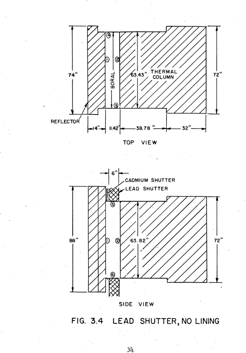
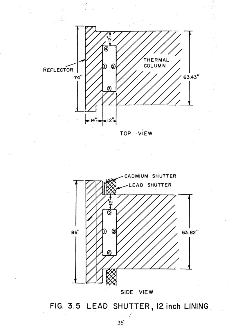
of putting a graphite lining on these edges. The model of the lead shutter region used in these calculations is shown in
figures 3.4 and 3.5. Figure 3.4 shows the relationship between the faces for the present situation, and figure 3.5 shows the case of a 12 inch graphite lining on the edges of the cavity
For both cases the source on face one is taken as
Source = [ inT 2 cos[l x i]cos[8 .1i]
(3-1)
V
861in.
86.l7n.
86.1in.
where S = total number of neutrons/sec emitted by the source x and y are the vertical and horizontal distances re-spectively from the center of face one to the position
(x,y) on face one.
2
Thus, the source in neutrons/cm -sec for a subarea with a side of length L is
Source (subarea) =
261n.
Xfcos( .10in )cos ( 1 0 in)dxdy
subarea 3.2)
-r
72"
38.78 32"TOP
VIEW
72ISIDE
VIEW
FIG. 3.4
LEAD SHUTTER, NO LINING
'p
REFLECTOR
TOP
-VIEW
SIDE
VIEW
FIG. 3.5 LEAD SHUTTER, 12 inch LINING
63.43"
For the case of no lining L is taken as 6.333 inches, and
for.
the case of 12 inch lining, L is taken as 3.911 inches.
In the case of no lining, two edges of the cavity are a
combination of air, cadmium, and lead.
In determining the
albedo for a subarea on one of these faces, air and cadmium are
assumed to have albedoes of zero; therefore, the albedo of the
subarea is the albedo of lead weighted by its area fraction.
The albedo for lead has been estimated using diffusion theory.
The other two edges of the cavity are boral. The albedos
for these edges are taken from Madell's thesis.
Shown in figure 3.6 is a plot of the centerline flux
across
face 2 (the face of the thermal column).
The upper curve
is the case of a 12 inch graphite lining on the edges of the
cavity, and the lower curve is the case of no lining. The
lining reduces the size of the cavity and the number of neutrons
entering it; however, the increase in albedo of the edges is so
great that there is a net increase in flux on the thermal
column face.
With no lining it is found that 68.7% of the neutrons
which enter the cavity are lost through the edges and 20.6%
are available for diffusion down the thermal column. The
remaining 10.7% are reflected back into the reflector of the
reactor. Heimberg analysed the same problem with a Monte
Carlo calculation and found that 29.3% of the neutrons
en-tering the cavity were available to the thermal column. The
difference between his value and the value of 20.6% found by
this model is due to the fact that he used lead on all four
12" GRAPHITE LINING
NO LINING
0
10
20
30
40
DISTANCE ACROSS FACE , INCHES
FLUX ACROSS
COLUMN FACE
CENTERLINE OF THERMAL
37
12r- I1t-10-9
1-8
1-7
h-6
E-E x DL-
431
--40
-30
-20
-10
FIG. 3.6
I
I
I
I
I5t--I
|
|I
I
|
|
I
i
i
edges of the cavity rather than boral on two edges and a mix-ture of lead, air, and cadmium on the other two edges. To
de-termine the effect of doing this, the problem was recalculated
by the view factor method using lead on all four edges. The number of neutrons available to the thermal column was found to be 30.5% which is in good.agreement with Heimberg's
value of 29.3%.
With the 12 inch graphite lining on the edges it is found that the leakage through these edges is reduced to 43.3% and the number of neutrons available to the thermal column in-creased to 28%. This fact along with the results of the ex-perimental investigation of the shielding effects of the lead shutter (Appendix C) indicate that it may be advantageous to eliminate the lead shutters and line the edges of the one foot cavity with graphite. The optimum thickness of this lining is discussed in the next chapter. A small gap will still have to be left for the cadmium shutter, and provisions made for the insertion of a temporary lead shield wherever it is necessary to work in the.hohlraum region.
Chapter 4
Optimization of Thermal Column
4.1 Empty Cavity
Shown in figure
4.1
is the thermal column with the
pro-posed cavity as described in section 2.1. Face 1 is the edge
of the graphite reflector surrounding the reactor and is the
source of neutrons.
The aim of this section is to determine the wall
thick-ness which will give the maximum thermal flux in the cavity.
Increasing the wall thickness increases its albedo and reduces
leakage from the cavity. From this it .can be concluded that
the maximum flux in .the cavity will occur when the wall
thick-ness is increased without limit.
However, since the outside
dimensions of the thermal column are fixed any increase in
wall thickness has to be done on the inside of the cavity.
This reduces the size of face 1 and the source of neutrons.
Consequently it might be expected that an increase in wall
thickness will result in a decrease in the flux in the cavity.
To determine the optimum wall thickness, the flux on
face 2 has been calculated for four different wall thicknesses:
zero inches, eight inches, 12 inches, and 16 inches.
For each
wall thickness, three end.condit-ions have been-used:
(a)
no end (face 2 albedo
=
0), which gives the lowest possible
flux; (b) infinite end (face 2 albedo
=
1), which gives the
high-est possible flux; and
(c) 32 .inches
of graphite, which .is the
actual situation.
I7
TOP
VIEW
-SIDE
VIEW
FIG. 4.1 MODIFIED THERMAL COLUMN
40
The source is the same as that used in the- lead shutter problem, section 3.2. The subarea sizes used in the various
cases are given in Table 4.1.
Table 4.1
Length of Subarea Edge
Wall Thickness, inches L, inches
0
6.333
8
6.061
12
5.633
16
6.308
Shown in figure 4.2 is a plot of the flux on face two as a function of wall thickness and end condition. Shown is both the average flux and the peak flux. The curves have been nor-malized to the average .flux for the case of no walls and no end. As is expected, for any wall thickness' the larger the albedo of face 2, the larger the flux. Also, the albedo of face 2 has a larger effect as the walls get thicker, because leakage out through the sides is smaller.
For the case of no end, the flux increases with wall thickness up to about 10 inches. At this point the reduction
in source due to thb reuluction in cavity size becomes impor-tant and the curve begins to decrease slightly. For the dases
of a 32 inch end and and infinite end, the flux continues to increase for wall thicknesses greater than 8 inches; however beyond 8 inches, the rate of increase drops off rapidly.
AVERAGE FLUX
PEAK FLUX
INFINITE ~~-0~~1-/
/
I/
32 INCH END NO END ---- 0 - - -0-- - - ---0
2
4
FIG..4
6
8
10
12
14
WALL THICKNESS, INCHES
.2
-
FLUX ON FACE 2
42
15
I
1I
9
x -J -J5
16
Since it would be desirable to have as much space as possible for the location of a large cold neutron cryostat, the walls should be kept as thin as possible. Thus, it can be concluded that the optimum wall thickness is about 8 inches.
4.2 Comparison with a Solid Thermal Column
Since the object of the hohlraum is to increase the thermal flux in the thermal column, the flux calculated for
face 2 should be compared with the flux at the same position in the present thermal column. The thermal column, shown in figure 3.4, can be considered in two.sections. From diffusion theory, the flux for each section can be written as,
Acos os Y[Ylz+K eYiz-,o<z<d (4.1) = Bcos _coslrysinhy (E-z), d<z<e (4.2)
2 c
where = extrapolated height of first section
5extrapolated width of first sectioh
d = length of first section
= extrapolated height and width of second section e = overall length of thermal column
e = extrapolated length of thermal column Y2
2
+(H)2
+ (.I)22 1
Y
2E2
+ 22)
A, B, and K are constants determined from the boundry 1
conditions,
$1i $2
at z
=d
- 2.Lat z
=d
$i = to at z = 0(4.3)
(4.4)
(4.5)
where $O is the flux on the face of the thermal column cal-culated in the lead shutter problem, Section 3.2.
Applying these. boundry conditions gives
(4.6)
-2yid 1
KI
=e Y
2Tanhy2(E-d)-lyi
2Tanh
y
2(-d) )+1
B = A( )2 e-Yid+Kieyid sin(U/E-l)f/2 + sin(Z/Ei+l)Tr/2
' sinhY2(5-d) V/E-1 /E+l
sin(U/5-l)ff/2 + sin(Z/U+l)ff/2
E/5-1 Z /5+1*
and
4 . rXai .f Wi . Yai
A =[
l+KI
i[sin. - sinE-]Xi[sin-5aa
a
5
where
.
= $ for the itfor he *th
subarea on the face(47)
.
rYii
-sin
I
(4.8)
thermal column
Xii, Yii = Lower limits Xai, Yai = Upper limits
of X and.'Y for of X and Y for a = 63.82 inches
b
=63.43
inches
c =
72.00 inchesd
=38.78
inches
e
=70.78
inches
7 = 65.24 inchesB
=
64.85
inches
E = 73.42 inches 9 = 71.149 inchesUsing,
ith
.thsubarea.
subarea.
L =
54.lcm.
Y:= 0.082885/in.
Y
2=0.076591/in.
gives
K = 5.2975 X 10-51
~-4
2.
A
=S(1.6388 X 10
)n/cm 'sec
S(9.7303 X 10- )n/cm
2sec.
where S is defined in Section 3.2.
Therefore, the flux in the thermal column can be written
as,
n Trx 7ry
S(1.6388 X 10~ cmz -sec)cos(65.24 in)cos (64.85in)
X[e0.082885z + 5.2975 X 10⁻⁵e0.082895z1,0<z<38.78in
= SC9.7-303 X 10 cm -sec)cos( 73.42in)Cos( 73.42in Xsinh[0.076591(71.49in-z)],38.78in<z<70.78in
(4.9) and the average flux at z =. 38.78 inches as
Tr
2SC2.8775 X 10 )n/cm *sec. (4.10)
The average flux at the same position (Face 2) of a cavity having eight inch thick walls is
=
S(9.3090
X 10- 5)n/cm2 -sec; (4.11)thus, the hohlraum increases the flux in the thermal column by a factor of 32.35.
4.3 Effect of Coolant Pipes
It is proposed to locate the coolant pipes of the reactor in the region presently occupied by the lead shutters, as shown
in figure
4.3.
COOLANT
PIPES
FIG. 4.3 LOCATION OF COOLANT PIPES
The pipes are eight inch diameter aluminum pipes and the coolant is light water.
The purpose of this section is to determine the effect of the pipes on the flux in the thermal column hohlraum.
To determine the effect of the coolant pipes it is
necessary to know the combined albedo of the light water and the aluminum. The albedo of the water is taken as
d
Bw
= 1-2~coth(t/L)
d
(4.12)
1+2f coth(t/L)
where D diffusion Coefficient = 0.141cm L = diffusion Length = 2.75
cm
t = thickness = 8 inches
the value of the water albedo becomes Bw =
0.81398.
Since the aluminum pipe is thin, .diffusion theory cannot be applied; however, the effect of the aluminum can be
con-servatively estimated by multiplying the albedo of the water. by the factor
e-2 tt (4.13)
where Et = total cross section =
0..09850/cm
t = pipe thickness = 5/16 inch
Application of this factor reduces the albedo to 0.69615. The case with 8 inch thick walls and a 32 inch thick end has been recalculated with the coolant pipes located as shown in figure 4.3. The average flux on face two has been found to be
=
S(8.6986
x 10-5)n/cm2 -sec (4.14) which is 6.55% lower than the case with no coolant pipes.4.4
Plane Object in Cavity
Up to this point, the calculations involving the op-timization of the thermal column have been limited to an
empty cavity. In the real situation the cold neutron cryostat will be located in the cavity. The purpose of this section is to investigate the effect of an object in the hohlraum on the flux in that region.
The model discussed in Chapter 2, with some modifications, is applicable to the special case of a two dimensional object
in a cavity. Although such a special case cannot give a true representation of the real situation, it can give in a simple manner some indication of how an object such as the cold
neutron cryostat will affect the flux in the thermal column cavity.
The model used for analysing the plane object problem is illustrated in figure 4.4. The- two dimensional plane object is oriented so that its faces are towards face 1 of cavity 1 and face 2 of cavity 2. The original, empty, cavity is di-vided into two cavities, the dividing plane being the one containing the two dimensional object. The fluxes on the su.r-faces of the cavities are calculated as follows.
The subareas on face 2 of cavity 1 that are covered by the plane object are assigned albedos corresponding to the
material of the object. The subareas not covered by the object are assigned fictitious albedos. With a source of neutrons at face 1, the fluxes on the surfaces of cavity.1 are calculated
0 00
FIG. 4.4 PLANE OBJECT IN. CAVITY
by the method described in Chapter 2.
Next the subareas on face 1 of cavity 2 that are covered by the plane object are assigned albedos corresponding to the material of the object, and the subareas that are not covered are assigned albedos of zero. Fictitious values are not used because neutrons incident on these subareas must be reflected in cavity 1 before they can re-enter cavity 2. However, this is the current incident on the part of face 2 cavity 1
that is not covered by the object and is taken as the source for cavity 2,
SOM(J1,Kl,2) = GM2(J2,K2,1) (4.15) where, SOM(Jl,Kl,2) = Source for a subarea located at
(Jl,Kl) on face 1 of cavity 2.
GM2(J2,K2,1) = Current incident on a subarea located at (J2,K2) on face 2 of cavity 1.
J2 = Jl, excluding area covered by object K2 = Kl, excluding area covered by object.
With this source the fli.xes on the surfaces of cavity 2 are calculated, again using the method of Chapter 2.
New fictitious albedos for face 2 of cavity 1 are then calaulated using
BM2(J2,K2,1) = GM1(Jl>Kll2) (4.16) GM2(J2)K2h)
where
BM2(J21K2,l)
=Albedo for a subarea located at
GMl(Jl,Kl,2)
(J2,K2) on face 2 of cavity 1
= Current incident on a subarea located on face 1 of cavity 2
peated until.the nique is carried TARGET, which is is described in In carrying considered: (1) and (2) a purely the walls of the end as 32 inches
solution converges.
This iterative tech-out on a digital computer using the program a modification to the program HOLCAV. TARGET Appendix B.out the calculations, two limiting cases are a purely reflecting object, albedo = 1;
absorbing object, albedo = 0. For both cases cavity are taken as ei-ght inches thick, the thi.ck, and the source the same as that used
in the lead shutter problem, Section 3.2.
Shown in figure 4.5 is a plot of the fluxes on the
sur-faces of the object as a function of the object size.
For
each case three curves are shown:
(1) the flux on the front
surface (facing the source),(2) the flux on the back surface
(away from the source), and (3) the average flux for both
surfaces.
In general the results are as expected. Introduction of
the object into the cavity causes the flux to become asymmetric;
that is, the flux is higher on the face towards the source than
on the face away from the source. This asymmetry becomes
greater as the object gets larger because increasing the size
of the object reduces the number of neutrons reaching cavity
2, and consequently the flux on the face away from the source.
GM2(J2,K2,1)
= Current incident on a subarea locatedat (J2,K2) on face 2 of cavity 1.
J2 = Jl, excluding area covered by object K2 = Kl, excluding area covered by object.
re-FLECTOR NT -n
01
-n
C 0z
2
C-n
_0m
0
CD
1, 1~O
30 40 50 70SIZE , PER CENT OF CAVITY CROSS SECTION
.- EMPTY CAVITYCENTER REFLECTOR, AVERAGE m m r c 7-0 0 0 0 0 100
Also, for the absorber the flux decreases monotonically with increasing size.
Probably the most interesting result is that for a re-flector the average flux drops less than 10% as the object size increases from zero to 100% of the cross sectional area of the cavity. Since the cold moderator will be heavy water which is a good scatterer, it will behave similarly to the reflector. This means that for a fixed wall thickness
changing the size of the cold moderator will have little ef-fect on the number of neutrons available for slowing down, but will affect the position at which they enter the cold neutron source.
4.5. Effect on Lattice Facility
As shown in figure 2.1, the lattice facility hohlraum is located at the end of the thermal column. Because of the na-ture of the experiments carried out in the latti-e facility, it is necessary that the cadmium ratio in the hohlraum be maintained as high as possible. Since removing graphite from the thermal column reduces the amount of moderator between the core and the hohlraum, it might be expected that the
cadmium ratio in this region will be reduced. The purpose of this section is to investigate the effect of the proposed thermal column cavity on the cadmium ratio in the lattice facility hohlraum.
Consider .an infinite slab of graphite. From diffusion theory, the epithermal and thermal fluxes in the slab can be
written as
*E EOe~ E (4- 17)
where
$EO = epithermal flux -at z = o
$TO
=thermal flux at z
=o
Y
E =
epithermal attenuation length
Y
T
=
thermal attenuation length.
Writing the cadmium ratio as
CR = 1 + (4.19) E gives CR(z) = 1 +
TO e
Xz
(4.20)FE0
or
[CR(z)-1]
=[CR leXz
(4.21)
CR = cadmium ratio at z =o.
In general, X can be determined from the neutron
dif-fusion properties of graphite; however, it is felt that a more
accurate estimate of the effect of the proposed cavity can be
obtained by evaluating X from existing data for the present
thermal column. These data are listed in Table 4.2.
The
cadmium ratio at z =
26 inches has been measured as part of
this work and is discussed in-Appendix D. Using these values,
X is found to be 0.046488/in.
Table
4.2
Measured Cadmium Ratios
z, inches
CR
Foil
O(core tank)
34(6)
Au1
dia.
10 mils
thick
26
111
Al-Au(0.072%), 30 mils
dia.,
1"
thick
84.78
1700(7)
Au,g dia., 10 mils
thick
Since the graphite will be removed from the thermal
column in conjunction with the installation of the new reactor
core, it is necessary to know CR for the new core. From
0