Worldwide Variation in Life-Span Sexual Dimorphism and Sex-Specific Environmental Mortality Rates

HAL Id: hal-02391019

https://hal.archives-ouvertes.fr/hal-02391019

Submitted on 3 Dec 2019

HAL is a multi-disciplinary open access

archive for the deposit and dissemination of

sci-entific research documents, whether they are

pub-lished or not. The documents may come from

teaching and research institutions in France or

abroad, or from public or private research centers.

L’archive ouverte pluridisciplinaire HAL, est

destinée au dépôt et à la diffusion de documents

scientifiques de niveau recherche, publiés ou non,

émanant des établissements d’enseignement et de

recherche français ou étrangers, des laboratoires

publics ou privés.

and Sex-Specific Environmental Mortality Rates

Anatoly Teriokhin, Elena Budilova, Frédéric Thomas, Jean-François Guégan

To cite this version:

Anatoly Teriokhin, Elena Budilova, Frédéric Thomas, Jean-François Guégan. Worldwide Variation

in Life-Span Sexual Dimorphism and Sex-Specific Environmental Mortality Rates. Human Biology,

Wayne State University Press, 2004, 76 (4), pp.623-641. �10.1353/hub.2004.0061�. �hal-02391019�

Sex-Specific Environmental Mortality Rates

ANATOLY T. TERIOKHIN,1,2_{ELENA V. BUDILOVA,}2_{FREDERIC THOMAS,}1_AND

JEAN-FRANCOIS GUEGAN1

Abstract In all human populations mean life span of women generally exceeds that of men, but the extent of this sexual dimorphism varies across different regions of the world. Our purpose here is to study, using global demographic and environmental data, the general tendency of this variation and local deviations from it. We used data on male and female life history traits and environmental conditions for 227 countries and autonomous terri-tories; for each country or territory the life-span dimorphism was defined as the difference between mean life spans of women and men. The general tendency is an increase of life-span dimorphism with increasing average male–female life span; this tendency can be explained using a demographic model based on the Makeham–Gompertz equation. Roughly, the life-span dimorphism increases with the average life span because of an increase in the duration of expressing sex- and age-dependent mortality described by the second (exponential) term of the Makeham–Gompertz equation. Thus we investigated the differences in male and female environmental mortality described by the first term of the Makeham–Gompertz equation fitted to the data. The general pattern that resulted was an increase in male mortality at the highest and lowest latitudes. One plausible explanation is that specific factors tied to extreme latitudes influence males more strongly than females. In particular, alcohol consumption increases with increasing latitude and, on the contrary, infection pressures increase with decreasing latitude. This find-ing agrees with other observations, such as an increase in male mortality excess in Europe and Christian countries and an increase in female mortality excess in Asia and Muslim countries. An increase in the excess of female mortality may be also due to increased maternal mortality caused by an increase in fertility. However, this relation is not linear: In regions with the highest fertility (e.g., in Africa) the excess of female mortality is smaller than in regions with relatively lower fertility (e.g., in Asia). A possible expla-nation of this phenomenon is an evolutionary adaptation of women to the pressures of extremely high fertility by means of some reduction of their maternal mortality.

1

Centre d’Etudes sur le Polymorphisme des Micro-Organismes, CEPM/UMR CNRS-IRD 9926, Institut de Recherches pour le De´veloppement, 911 Avenue Agropolis, B.P. 64501, 34394 Montpellier Ce´dex 5, France.

2_{Chair of General Ecology, Faculty of Biology, Moscow State University, Moscow 119899, Russia.}

Human Biology, August 2004, v. 76, no. 4, pp. 000–000

Copyright䉷 2004 Wayne State University Press, Detroit, Michigan 48201-1309 KEY WORDS: SEXUAL DIMORPHISM, LIFE SPAN, MORTALITY RATE.

The existence of life-span sexual dimorphism in humans, characterized by a longer female life expectancy, is commonly recognized and empirically con-firmed (e.g., Lopez and Ruzicka 1983; Gavrilov and Gavrilova 1991; Trovato and Lalu 1998; Mathers et al. 2001; Kraemer 2000; Lobmayer and Wilkinson 2000; Kirkwood 2001; Luy 2002). However, there is no established consensus concern-ing the general worldwide pattern and regional deviations in differences between female and male life spans. Here, we address this question by analyzing global demographic and environmental data.

Evolutionary hypotheses explaining the emergence of female life-span pre-dominance are mainly based on the differences in ecological roles between males and females. Males are expected to maximize their fitness by increasing their mating success, whereas females need to increase their longevity for obtaining maximal reproductive output (Bateman 1948; Williams and Williams 1957; Rolff 2002). An evolutionary optimization model, based on the similar assumption that males should preferentially spend large amounts of energy in short times (mat-ing, hunting) and females should accumulate energy over long periods (gestation and rearing children), results in the emergence of greater female life spans (Teri-okhin and Budilova 2000). This ‘‘maternal’’ hypothesis can be completed by the ‘‘grandmaternal’’ hypothesis, which explains both extended female longevity and limited reproductive period (menopause) by advantages of grandmaternal care over maternal care for older females (Hamilton 1964; Trivers 1972; Alvarez 2000; Peccei 2001), and is partly confirmed by the analysis of observed data (Jamison et al. 2002; Sear et al. 2002; Voland and Beise 2002). Although children can inherit up to twice as many of the female’s genes as grandchildren, the risks for an old female not to have enough vital resources and time to gestate and bring up her own child would overcome the advantages of giving a new birth (Teriok-hin and Budilova 2000).

A quasi-universal predominance of female life expectancy and especially its persistence in highly developed countries, where differences in ecological roles of males and females are attenuated and environmental mortality risks are reduced, suggest that a substantial component of the sex difference in life expec-tancy is under genetic control (Wells 2000). We refer to this as life-span sexual dimorphism. However, nongenetic external causes of mortality that affect males and females differently, which we call sex-specific environmental mortality, un-doubtedly exist. For example, the consumption of alcohol, usually higher in males, is known to reduce the life span of males (Lunetta et al. 1998; Nolte et al. 2003). Some studies argue that males are more vulnerable to infections (Frances-chi et al. 2000; Wells 2000). In contrast, environmental conditions, primarily social ones, might reduce the longevity of females (Klasen 1998; Lavoyin 2001). We used the Gompertz–Makeham model (Gompertz 1825; Makeham 1860) to divide total mortality into two components: one that reflects the general tendency of age- and sex-dependent mortality and one that takes into account regional deviations (which, in addition, might be sex-specific) from this general tendency.

Materials and Methods

The global demographic and environmental data used in the analyses were collected for 227 countries and autonomous territories (see Appendix) using mainly international electronic databases accessible on the Internet, such as those provided by the World Health Organization (http://www.who.int), the Centers for Disease Control and Prevention in the United States (http://www.cdc.gov), the United Nations Statistical Division (http://un.stats.un.org), the World Bank Group (http://www.worldbank.org), and the World Sites Atlas (http://www.sites-atlas.com). These data were partly completed by information from other sources (e.g., scientific journals and reports from ministries of health).

Disease occurrences in the different countries were compiled for a set of 324 categories of human parasitic and infectious diseases affecting human sur-vival (see more information at http://www.cyinfo.com), and the disease load was calculated as the total number of diseases for each country. The consumption of alcohol per individual was measured in liters per capita per year. Life expectancy at birth and infant mortality were considered separately for each sex. The mater-nal mortality ratio was defined as the number of matermater-nal deaths caused by deliv-eries and complications of pregnancy and childbirth divided by the number of live births for a given year; it is expressed per 100,000 live births. The fertility indicates the number of offspring born to a woman per lifetime passing through the child-bearing age. The nutritional conditions were evaluated by the calorie consumption per average inhabitant per day. Mean latitude and mean longitude refer to the value measured at the geographic center of each country.

Instead of life span at birth L0, which is presented in our source data and

which includes infant mortality of the first year of life, we use the life-span estimate L1, which is calculated under the assumption of having survived the first

year. L1can be obtained from the equation representing L0as a weighted sum of

L⬍1(the life span of those who have not survived the first year) and L1(the life

span of those who did survive the first year):

L0⳱ p1L⬍1Ⳮ (1 ⳮ p1)L1, (1)

where p1is the probability of dying during the first year, which is also present in

our data. Taking into account that L⬍1is equal to 1ⳮ p1(the probability of

sur-viving the first year), we obtain the following formula for L1:

L1⳱

L0

(1ⳮ p1)

ⳮ P1. (2)

The values of L1were calculated separately for women and men using the values

of L0and p1 (known for each sex). Only values of L1will be used further and

Figure 1. Scatterplots and regression lines of female (upper) and male (lower) life spans on aver-age life span (female–male mean life-span half-sum).

Regression and variance analyses were performed using the S-Plus statisti-cal package (Venables and Ripley 1994).

General Tendency of Life-Span Dimorphism. The general tendency of the global pattern of life-span dimorphism is that dimorphism increases with the average life span (half-sum of female and male mean life spans). This appears clearly in Figure 1, where the dependencies of female and male life spans, Lfand Lm, on their half-sum L are approximated by the linear regressions

Lf⳱ ⳮ1.822 Ⳮ 1.0641L, R⳱ 0.996, p ⬍ 0.0000001, (3)

and

Lm⳱ 1.822 Ⳮ 0.9349L, R⳱ 0.996, p ⬍ 0.0000001. (4)

In more detail, this tendency is shown in Figure 2, where the dependence of life-span dimorphism, defined as female minus male life life-span, d⳱ Lfⳮ Lm, on L is

Figure 2. Scatterplots and regression line of female minus male life span on average life span (female–male mean life-span half-sum).

d⳱ ⳮ3.644 Ⳮ 0.128L, R⳱ 0.564, p ⬍ 0.0000001 (5)

(country names are designated by their two-letters codes, given in the Appendix). Alternatively, the significance of increasing life-span dimorphism with in-creasing life span can be detected using an approach proposed by Mosimann (Mosimann 1970; Mosimann and Darroch 1985). According to this approach, we should regress the logarithms of Lf on the averages of the logarithms of Lf

and Lm and compare the slope of this regression with 1.0. In our case we

ob-tained a value of slope equal to 1.039, which is significantly greater than 1.0 (p⬍ 0.0000001), thus indicating that life-span dimorphism does increase with increasing life span.

This tendency can be explained by using the Gompertz–Makeham law (Gompertz 1825; Makeham 1860), which presents the age dynamics of the indi-vidual rate of mortality m(t) as the sum of two terms, according to the following equation:

The first term, A, is independent of age and reflects the action of environmental causes of death, whereas the second term increases exponentially with age t. The accelerated increase of mortality with age can be explained by a progressive reduction of an organism’s resources allocated to its repair, as is predicted by evolutionary optimization models (Abrams and Ludwig 1995; Cichon 1997; Teri-okhin 1998).

The estimations of the parameters A, B, and C from demographic data for different human populations (e.g., Gavrilov and Gavrilova 1991) show that parameters B and C are relatively stable in geographic space and historical time compared to parameter A and that parameter C is more stable with respect to sex. We therefore assume the following model to describe the age dynamics of the mortality rate m(r, s, t) for an individual of sex s (f, female; m, male) living in a region r:

m(r,s,t)⳱ ArⳭ BseCt. (7)

When the age dynamics of mortality are known, the individual’s expected mean life span can be computed using the equation

Ls⳱ 1 Ⳮ

冘

冋

册

which approximates the exact integral equation

Ls⳱1 Ⳮ

冕

冋

册

The maximum life span T in the approximated equation must be a sufficiently large age for which the probability to survive up to it is small. We used the value

T⳱ 120, for which this probability is less than 0.0000001, even in the absence

of environmental mortality.

To find the best estimates for the parameters Bf, Bm, and C (i.e., minimizing

the sum of squares of differences between observed and estimated life spans through all the countries and both sexes), we assumed that on the global scale the regional sex differences in the parameter Arare mutually balanced (i.e., that

the values of the parameter Arfor each region r were equal for both sexes). Thus

we had to estimate NⳭ 3 parameters on the basis of 2N observations (life spans for males and females for N countries).

The estimates obtained for the parameters were Bf⳱ 0.0000078, Bm⳱ 0.000017, and C ⳱ 0.101. In turn, the estimates of life spans computed

using the Gompertz–Makeham equation with these parameter estimates (plus corresponding estimates of Ar) do not differ practically (not greater than

the observed linear trend of life-span dimorphism associated with increasing av-erage life span can be explained by sex differences in the parameter Bs in the

Gompertz–Makeham equation.

Regional Deviations from the General Tendency. We then tried to explain the deviations from the general linear trend by using the regional differences in the first term of this equation:

m(r,s,t)⳱ Ar,sⳭ BseCt. (10)

In this second stage of the analysis, values of parameters Bf, Bm, and C were fixed

at their estimated values and parameter A was allowed to depend both on region and sex. Fitting this model to the data allowed us to estimate values of environ-mental mortality rate for each country and for each sex (see Appendix). We then tried to relate mortality sex-specific differences, expressed by Ar,s, to the

environmental conditions in different countries. To attenuate the role of outlying differences between male and female environmental mortality rates, we did not analyze row differences but their logarithmically transformed values dA, obtained

using the equation

dA⳱ Ⳳ(Ar, mⳮ Ar, f)log[1Ⳮ 10,000兩(Ar, mⳮ Ar, f)兩], (11)

which we call male environmental mortality rate excess, or simply male mortal-ity excess.

To evaluate the environmental influence on sexual differences in environ-mental mortality, we estimated the dependencies of dAon different

environmen-tal factors using regression and dispersion analyses.

These analyses identified several environmental factors significantly re-lated to dA ,some of which were nonlinear. In particular, the excess of male

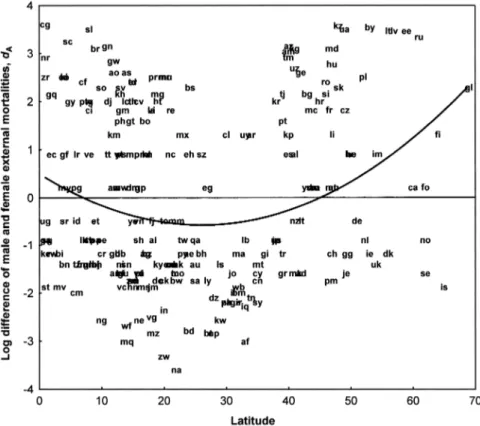
environmental mortality is observed at lower and higher latitudes (lesser than 10⬚ and greater than 45⬚; see Figure 3). The dependence of dAon latitude x is

de-scribed by a second-order polynomial function with a statistically significant qua-dratic term:

dA⳱ 0.4574 ⳮ 0.07736x Ⳮ 0.001499x2,

R⳱ 0.225, px⳱ 0.0037, px2⳱ 0.00048. (12)

We suggest that such a nonlinear dependence can be explained by opposite linear dependences of drwith different environmental factors. Factors significantly (at

the 5% level) related to the male mortality excess are shown in Tables 1 and 2. From Table 1 we see that the factor that is the most incontestably correlated with dA(R⳱ 0.27, p ⳱ 0.00024) is the annual per capita consumption of alcohol.

This factor is also positively correlated with latitude (R⳱ 0.50, p ⬍ 0.0000001), so that the excess of male environmental mortality at higher latitudes can, at least

Figure 3. Scatterplots and quadratic regression line of excess of male environmental mortality dA

(see text) on latitude. Names of regions (countries and autonomous territories) are indi-cated by their two-letter codes (see Appendix).

Table 1. Quantitative Environmental Factors Significantly Correlated to the Excess of Male Environmental Mortality, dA

Environmental Factor Correlation with dA p Level for Testing H0: R⳱ 0

Alcohol 0.27 0.00024

Infections 0.19 0.013

Physicians 0.22 0.0034

in part, be explained by a negative influence of excessive consumption of alcohol, which affects primarily men (Lunetta et al. 1998; Nolte et al. 2003). On the contrary, another environmental factor, the number of infections (corrected for the logarithm of population number), which also correlated positively with

dA (R⳱ 0.19, p ⳱ 0.013) (see Table 1), increases with decreasing latitude

(R⳱ ⳮ0.53, p ⬍ 0.0000001). This may explain, at least in part, the increase in male mortality excess at lower latitudes, because, in general, infections affect men more strongly than women (Franceschi et al. 2000; Wells 2000). We might

Table 2. Qualitative Environmental Factors Significantly Related to the Excess of Male Environmental Mortality, dA

Mean Values of dA p Level for Testing the

Environmental Factor in Presence and Absence of Factor Absence of Difference

Europe 0.50 vs.ⳮ028 0.011

Asia ⳮ0.49 vs. 0.05 0.044

Muslims ⳮ1.07 vs. ⳮ0.19 0.0088

Christians ⳮ0.16 vs. ⳮ0.74 0.048

Island ⳮ0.48 vs. 0.05 0.044

generalize these two observations by proposing that stressful factors, in particu-lar, those manifested at extreme higher and lower latitudes, influence primarily men negatively, thus increasing the excess of male environmental mortality (Wells 2000).

The same line of thinking can be applied to the negative correlation of insular situation of region with dA(mean value of dAisⳮ0.48 on islands versus

0.05 on continents, p⳱ 0.044) (see Table 2). We suggest that stressful factors on islands are less expressed than on continental territories. The correlation of dA

with the number of physicians may simply be due to its correlation with other environmental factors, in particular, with alcohol (R⳱ 0.57, p ⬍ 0.0000001). Di-rect interpretation of this correlation (i.e., that women are more sensitive to an increase or decrease in the number of physicians) is nevertheless also possible.

The significant effect of continent and religion (dA is higher in European

and Christian countries and lower in Asian and Muslim countries; see Table 2) can also be explained by the influence of some environmental factors. Indeed, the consumption of alcohol is significantly greater in Europe than in Asia (11.1 versus 2.8 l, p⬍ 0.0000001) and in Christian countries than in Muslim countries (7.3 versus 0.9 l, p⬍ 0.0000001).

An additional factor that lowers the excess of male environmental mortality (or rather, increases the excess of female environmental mortality) in Muslim countries compared with Christian countries is higher fertility (4.4 versus 2.8 children, p⳱ 0.000014). Higher fertility may decrease dAbecause of

increas-ing maternal mortality, which is strongly correlated with fertility (R⳱ 0.80,

p⬍ 0.0000001).

However, the relation of excess male environmental mortality with fertility is not linear. We see in Figure 4 that, although male mortality excess decreases with increasing fertility from lowest to middle values (from 1 to 4.5 children), dA

increases with increasing fertility from middle to highest values (from 4.5 to 8 children). The dependence of dAon fertility f is well described by a second-order

polynomial function with a statistically significant quadratic term:

dA⳱ 2.139 ⳮ 1.278f Ⳮ 0.1467f2,

Figure 4. Scatterplots and quadratic regression line of excess of male environmental mortality dA

(see text) on fertility. Names of regions (countries and autonomous territories) are indi-cated by their two-letter codes (see Appendix).

One interpretation of a relative increase in dA at low latitudes is based on the

fact that fertility, like infections, significantly increases with decreasing latitude (R⳱ ⳮ0.62, p ⬍ 0.0000001). However, we have already noted a negative influ-ence of the infection pressure on males. If this pressure overcomes the negative effect of high fertility, which acts predominantly negatively on females, it may explain the observed increase in dAin regions with highest fertility.

The increase in dAwith increasing fertility (in parallel with increasing

in-fections) to its highest value can also be explained by evolutionary adaptation of women to the necessity of having a considerable increase in fertility in relation to a high parasitic pressure (Gue´gan and Teriokhin 2000; Gue´gan et al. 2000). In support of this, the highest fertility values are mainly observed in Africa (5.1 children in Africa versus 3.3 in Asia and 1.4 in Europe), where the average life span is extremely low (53.1 years in Africa versus 69.2 in Asia and 76.1 in Europe). Thus a relative reduction in female environmental mortality (by means

of genetic selection or cultural adaptation) may indeed be vitally important for population survival.

Conclusion

The two goals of this study were (1) to identify and explain the general tendency of human life-span sexual dimorphism and (2) to identify and relate the deviations from the general tendency to environmental conditions.

The general tendency consists in an increase of life-span dimorphism with improved environmental conditions and an increase in mean life span. This tendency is observed empirically and can be obtained theoretically if we assume that the age-dependent exponential component of human mortality in the Gompertz–Makeham equation is more conservative than the age-independent (but environment-dependent) component. On the intuitive level this increase in life-span dimorphism with increasing average male–female life span is due to the fact that the longer the life span of men and women, the longer the period for expressing the difference in their age-dependent mortalities.

With regard to deviations from the general trend, the general pattern indi-cates an excess of male mortality at the highest and lowest latitudes. One expla-nation is that the stressful factors linked to extreme latitudes affect males more strongly than females. In particular, alcohol consumption increases with increas-ing latitude and infection pressures increase with decreasincreas-ing latitude. This pattern agrees with observations that male environmental mortality increases in Euro-pean and Christian countries and that female mortality increases in Asian and Muslim countries. An increase in the excess of female mortality might also be caused by increased maternal mortality associated with increasing fertility, al-though this relation is not linear. However, in the regions with highest fertility, notably in Africa, the excess of female mortality is lower than in Asia. A possible explanation may be that African populations have adapted to their highly stressful environment by means of female mortality reduction.

Acknowledgments We thank B. Lafay for helpful comments and an anonymous ref-eree for numerous valuable suggestions. The research was supported by the Centre Na-tional de la Recherche Scientifique (CNRS) through a Senior Research Fellowship awarded to A. Teriokhin and by funds from the Russian Foundation for Basic Research (RFBR) (grant 01-04-48384) awarded to E. Budilova and A. Teriokhin.

Received 23 March 2003; revision received 29 October 2003.

Literature Cited

Abrams, P.A., and D. Ludwig. 1995. Optimality theory, Gompertz’ law, and disposable soma theory of senescence. Evolution 49:1,055–1,056.

Alvarez, H.P. 2000. Grandmother hypothesis and primate life histories. Am. J. Phys. Anthropol. 113:435–450.

Bateman, A.J. 1948. Intra-sexual selection in Drosophila. Heredity 2:349–368.

Cichon, M. 1997. Evolution of longevity through optimal resource allocation. Proc. R. Soc. Lond. B 264:1,383–1,388.

Franceschi, C., L. Motta, S. Valensin et al. 2000. Do men and women follow different trajectories to reach extreme longevity? Aging Clin. Exp. Res. 12:77–84.

Gavrilov, L.A., and N.S. Gavrilova. 1991. The Biology of Life Span: A Quantitative Approach. New York: Harwood Academic.

Gompertz, B. 1825. On the nature of the function expressive of the law of human mortality and on a new mode of determining life contingencies. Phil. Trans. R. Soc. Lond. A 115:513–585. Gue´gan, J.F., and A.T. Teriokhin. 2000. Human life-history traits on a parasitic landscape. In

Evolu-tionary Biology of Host–Parasite Relationships: Theory Meets Reality, R. Poulin, S. Morand,

and A. Skorping, eds. Amsterdam: Elsevier, 143–161.

Gue´gan, J.F., A.T. Teriokhin, and F. Thomas. 2000. Human fecundity variation, size-related obstetrical performance, and the evolution of sexual stature dimorphism. Proc. R. Soc. Lond. B 267:2,529–2,536.

Hamilton, W.D. 1964. The genetical evolution of social behavior. J. Theor. Biol. 7:1–16.

Jamison, C.S., L.L. Cornell, P.L. Jamison et al. 2002. Are all grandmothers equal? A review and a preliminary test of the grandmother hypothesis in Tokugawa, Japan. Am. J. Phys. Anthropol. 119:67–76.

Kirkwood, T.B.L. 2001. Sex and aging. Exp. Gerontol. 36:413–418.

Klasen, S. 1998. Marriage, bargaining, and intrahousehold resource allocation: Excess female mortal-ity among adults during early German development, 1740–1860. J. Econ. Hist. 58:432–467. Kraemer, S. 2000. The fragile male. Br. Med. J. 321:1,609–1,612.

Lavoyin, T.O. 2001. Risk factors for infant mortality in a rural community in Nigeria. J. R. Soc.

Prom. Health. 121:114–118.

Lobmayer, P., and R. Wilkinson. 2000. Income, inequality, and mortality in 14 developed countries.

Sociol. Health Illness 22:401–414.

Lopez, A.D., and L.T. Ruzicka, eds. 1983. Sex Differentials in Mortality: Trends, Determinants, and

Consequences. Canberra: Australian National University.

Lunetta, P., A. Penttila, and S. Sarna. 1998. Water traffic accidents, drowning, and alcohol in Finland, 1969–1995. Int. J. Epidemiol. 27:1,038–1,043.

Luy, M. 2002. Sex differences in mortality: Time to take a second look. Z. Gerontol. Geriatr. 35:412– 429.

Makeham, W.M. 1860. On the law of mortality and the construction of annuity tables. J. Inst.

Actuar-ies 8:301–310.

Mathers, C.D., R. Sadana, J.A. Salomon et al. 2001. Healthy life expectancy in 191 countries. Lancet 357:1,685–1,691.

Mosimann, J.E. 1970. Size allometry: Size and shape variables with characterization of the log nor-mal and generalized gamma distributions. J. Am. Stat. Assoc. 65:930–945.

Mosimann, J.E., and J.N. Darroch. 1985. Canonical and principal components of shape. Biometrika 72:241–252.

Nolte, E., A. Britton, and M. McKee. 2003. Trends in mortality attributable to current alcohol con-sumption in East and West Germany. Soc. Sci. Med. 56:1,385–1,395.

Peccei, J.S. 2001. A critique of the grandmother hypothesis: Old and new. Am. J. Hum. Biol. 13:434– 452.

Rolff, J. 2002. Bateman’s principle and immunity. Proc. R. Soc. Lond. B 269:867–872.

Sear, R., F. Steele, I.A. McGregor et al. 2002. The effect of kin on child mortality in rural Gambia.

Demography 39:43–63.

Slatkin, M. 1984. Ecological causes of sexual dimorphism. Evolution 38:622–630.

Teriokhin, A.T. 1998. Evolutionarily optimal age schedule of repair: Computer modeling of energy allocation between current and future survival and reproduction. Evol. Ecol. 12:291–307.

Teriokhin, A.T., and E.V. Budilova. 2000. Evolutionarily optimal networks for controlling energy allocation to growth, reproduction, and repair in men and women. In Artificial Neural

Net-works: Application to Ecology and Evolution, S. Lek and J.F. Gue´gan, eds. Berlin: Springer

Verlag, 225–237.

Trivers, R.L. 1972. Parental investment and sexual selection. In Sexual Selection and the Descent of

Man, 1871–1971, B. Campbell, ed. Chicago: Aldine, 136–179.

Trovato, F., and N.M. Lalu. 1998. Contribution of cause-specific mortality to changing sex differences in life expectancy: Seven nations case study. Soc. Biol. 45:1–20.

Venables, W.N., and B.D. Ripley. 1994. Modern Applied Statistics with S-Plus. Berlin: Springer-Verlag.

Voland, E., and J. Beise. 2002. Opposite effects of maternal and paternal grandmothers on infant survival in historical Krummhorn. Behav. Ecol. Sociobiol. 52:435–443.

Wells, J.C.K. 2000. Natural selection and sex differences in morbidity and mortality in early life. J.

Theor. Biol. 202:65–76.

Williams, G.C., and D.C. Williams. 1957. Natural selection of individually harmful social adaptation among sibs with special references to social insects. Evolution 11:32–39.

Appendix. Regions (Countries and Autonomous Territories)

Female Male Difference Environ- Environ- of Male Female Male mental mental and

Life Life Mortality, Mortality, Female Region (Country, Territory), r Code Span, Lf Span, Lm Ar,f Ar,m Mortalities

Afghanistan af 46.49 48.02 0.0166 0.0142 ⳮ0.0024

Albania al 75.41 69.55 0.0037 0.0038 0.0001

Algeria dz 71.93 69.15 0.0048 0.0039 ⳮ0.0009

Andorra ad 86.61 80.62 0.0005 0.0001 ⳮ0.0004

Angola ao 40.89 38.38 0.0205 0.0215 0.0010

Anguilla (United Kingdom) ai 79.63 73.83 0.0024 0.0023 ⳮ0.0001 Antigua and Barbuda ag 73.57 68.90 0.0043 0.004 ⳮ0.0003 Antilles (Netherlands) an 77.54 73.05 0.003 0.0025 ⳮ0.0005 Argentina ar 79.15 72.23 0.0026 0.0028 0.0002 Armenia am 71.38 62.55 0.005 0.0066 0.0016 Aruba (Netherlands) aw 82.23 75.37 0.0017 0.0017 0.0000 Australia au 83.04 77.19 0.0015 0.0011 ⳮ0.0004 Austria at 81.34 74.88 0.0019 0.0019 0.0000 Azerbaijan az 68.07 59.29 0.0062 0.0081 0.0019 Bahamas bs 73.60 66.45 0.0043 0.00 50.0007 Bahrain bh 76.08 71.21 0.0035 0.0032 ⳮ0.0003 Bangladesh bd 61.14 61.50 0.0089 0.0071 ⳮ0.0018 Barbados bb 76.20 70.99 0.0035 0.0033 ⳮ0.0002 Belarus by 74.65 62.40 0.0039 0.0067 0.0028 Belgium be 81.65 74.84 0.0018 0.0019 0.0001 Belize bz 74.02 69.36 0.0041 0.0039 ⳮ0.0002 Benin bj 51.03 49.26 0.0138 0.0134 ⳮ0.0004

Bermuda (United Kingdom) bm 79.33 75.29 0.0025 0.0018 ⳮ0.0007

Bhutan bt 53.40 54.09 0.0126 0.0107 ⳮ0.0019

Bolivia bo 67.46 62.24 0.0064 0.0067 0.0003

Bosnia and Herzegovina ba 75.08 69.48 0.0038 0.0038 0.0000

Botswana bw 35.64 35.38 0.025 0.0244 ⳮ0.0006 Brazil br 68.13 59.63 0.0062 0.0079 0.0017 Brunei bn 76.64 71.81 0.0033 0.003 ⳮ0.0003 Bulgaria bg 75.31 68.09 0.0037 0.0043 0.0006 Burkina Faso bf 47.24 45.95 0.0161 0.0156 ⳮ0.0005 Burundi bi 47.12 45.42 0.0162 0.0159 ⳮ0.0003 Cambodia kh 59.84 55.19 0.0095 0.0101 0.0006 Cameroon cm 55.58 53.90 0.0115 0.0108 ⳮ0.0007 Canada ca 83.29 76.34 0.0014 0.0014 0.0000 Cape Verde cv 73.24 66.61 0.0044 0.0049 0.0005 Cayman Islands ky 81.66 76.47 0.0018 0.0014 ⳮ0.0004 (United Kingdom)

Central African Republic cf 45.56 42.54 0.0172 0.018 0.0008

Chile cl 79.69 72.90 0.0024 0.0026 0.0002

China cn 74.08 70.19 0.0041 0.0035 ⳮ0.0006

Colombia co 74.97 67.18 0.0038 0.0047 0.0009

Comoros km 63.54 59.09 0.0079 0.0082 0.0003

Congo, Brazzaville cg 51.71 44.72 0.0135 0.0164 0.0029 Congo Democratic Republic zr 51.58 47.69 0.0135 0.0144 0.0009

Female Male Difference Environ- Environ- of Male Female Male mental mental and

Life Life Mortality, Mortality, Female Region (Country, Territory), r Code Span, Lf Span, Lm Ar,f Ar,m Mortalities

Cook Islands (New Zealand) ck 73.25 69.39 0.0044 0.0038 ⳮ0.0006

Costa Rica cr 78.97 73.77 0.0026 0.0023 ⳮ0.0003 Cote d’Ivoire ci 46.41 43.88 0.0166 0.017 0.0004 Croatia hr 78.01 70.58 0.0029 0.0034 0.0005 Cuba cu 79.20 74.26 0.0025 0.0021 ⳮ0.0004 Cyprus cy 79.54 74.84 0.0024 0.0019 ⳮ0.0005 Czech Republic cz 78.69 71.50 0.0027 0.0031 0.0004 Denmark dk 79.71 74.34 0.0024 0.0021 ⳮ0.0003 Djibouti dj 54.01 50.26 0.0123 0.0128 0.0005 Dominica dm 76.96 71.13 0.0032 0.0032 0.0000 Dominican Republic do 76.14 71.83 0.0035 0.003 ⳮ0.0005 Ecuador ec 74.77 69.05 0.0039 0.004 0.0001 Egypt eg 66.61 62.33 0.0067 0.0067 0.0000 El Salvador sv 74.29 66.92 0.0041 0.0048 0.0007 Equatorial Guinea gq 56.97 52.76 0.0108 0.0114 0.0006 Eritrea er 59.52 54.52 0.0096 0.0104 0.0008 Estonia ee 76.39 64.12 0.0034 0.0059 0.0025 Ethiopia et 45.50 43.81 0.0172 0.0171 ⳮ0.0001

Faeroe Islands (Denmark) fo 82.25 75.34 0.0017 0.0017 0.0000

Fiji Islands fj 71.20 66.23 0.0051 0.0051 0.0000 Finland fi 81.55 74.13 0.0019 0.0022 0.0003 France fr 83.17 75.21 0.0014 0.0018 0.0004 Gabon ga 50.66 48.50 0.0141 0.0139 ⳮ0.0002 Gambia gm 56.39 52.45 0.0111 0.0116 0.0005 Gaza Strip gz 72.69 70.13 0.0046 0.0036 ⳮ0.0010 Georgia ge 68.63 61.54 0.006 0.007 0.0010 Germany de 81.12 74.68 0.002 0.002 0.0000 Ghana gh 58.79 56.01 0.01 0.0097 ⳮ0.0003

Gibraltar (United Kingdom) gi 82.29 76.42 0.0017 0.0014 ⳮ0.0003

Greece gr 81.53 76.22 0.0019 0.0015 ⳮ0.0004

Greenland (Denmark) gl 72.43 65.25 0.0047 0.0055 0.0008

Grenada gd 66.41 62.83 0.0068 0.0065 ⳮ0.0003

Guadeloupe (France) gp 80.72 74.27 0.0021 0.0021 0.0000 Guam (United States) gu 80.77 75.86 0.0021 0.0016 ⳮ0.0005

Guatemala gt 69.94 64.47 0.0055 0.0058 0.0003

Guernsey (United Kingdom) gg 83.05 76.95 0.0015 0.0012 ⳮ0.0003

Guinea gn 49.38 44.41 0.0148 0.0167 0.0019 Guinea-Bissau gw 52.70 48.03 0.0129 0.0142 0.0013 Guyana gy 65.56 60.21 0.0071 0.0076 0.0005 Guyana (France) gf 80.09 73.26 0.0023 0.0025 0.0002 Haiti ht 51.72 48.36 0.0135 0.014 0.0005 Honduras hn 70.71 67.33 0.0053 0.0046 ⳮ0.0007

Hong Kong (China) hk 82.74 77.14 0.0015 0.0012 ⳮ0.0003

Hungary hu 76.61 67.62 0.0033 0.0045 0.0012

Appendix. (Continued)

Female Male Difference Environ- Environ- of Male Female Male mental mental and

Life Life Mortality, Mortality, Female Region (Country, Territory), r Code Span, Lf Span, Lm Ar,f Ar,m Mortalities

India in 64.31 62.93 0.0076 0.0064 ⳮ0.0012 Indonesia id 71.33 66.50 0.005 0.005 0.0000 Iran ir 71.88 69.07 0.0049 0.004 ⳮ0.0009 Iraq iq 68.85 66.73 0.0059 0.0049 ⳮ0.0010 Ireland ie 80.16 74.45 0.0023 0.002 ⳮ0.0003 Israel il 81.06 76.88 0.002 0.0012 ⳮ0.0008 Italy it 82.67 76.13 0.0016 0.0015 ⳮ0.0001 Jamaica jm 77.83 73.76 0.003 0.0023 ⳮ0.0007 Japan jp 84.28 77.76 0.0011 0.001 ⳮ0.0001

Jersey (United Kingdom) je 81.44 76.38 0.0019 0.0014 ⳮ0.0005

Jordan jo 80.42 75.43 0.0022 0.0017 ⳮ0.0005 Kazakhstan kz 69.38 58.39 0.0057 0.0085 0.0028 Kenya ke 48.15 46.52 0.0155 0.0152 ⳮ0.0003 Kiribati ki 63.92 57.94 0.0078 0.0087 0.0009 Kuwait kw 77.46 75.65 0.0031 0.0016 ⳮ0.0015 Kyrgyzstan kg 68.42 59.85 0.0061 0.0078 0.0017 Laos la 56.31 52.47 0.0111 0.0115 0.0004 Latvia lv 75.26 63.24 0.0038 0.0063 0.0025 Lebanon lb 74.50 69.59 0.004 0.0038 ⳮ0.0002 Lesotho ls 48.16 46.70 0.0155 0.0151 ⳮ0.0004 Liberia lr 53.98 51.02 0.0123 0.0124 0.0001 Libya ly 78.31 73.93 0.0028 0.0022 ⳮ0.0006 Liechtenstein li 82.77 75.52 0.0015 0.0017 0.0002 Lithuania lt 75.69 63.64 0.0036 0.0061 0.0025 Luxembourg lu 81.01 74.24 0.002 0.0021 0.0001 Macao (China) mo 84.77 79.00 0.001 0.0006 ⳮ0.0004 Macedonia mk 76.77 72.11 0.0033 0.0029 ⳮ0.0004 Madagascar mg 58.53 53.93 0.0101 0.0107 0.0006 Malawi mw 37.57 36.50 0.0233 0.0233 0.0000 Malaysia my 74.33 68.90 0.004 0.004 0.0000 Maldives mv 64.60 62.09 0.0075 0.0068 ⳮ0.0007 Mali ml 49.18 46.76 0.0149 0.015 0.0001 Malta mt 81.00 75.82 0.002 0.0016 ⳮ0.0004

Man, Isle of (United Kingdom) im 81.40 74.49 0.0019 0.002 0.0001 Marshall Islands mh 68.34 64.61 0.0061 0.0057 ⳮ0.0004 Martinique (France) mq 78.00 79.23 0.0029 0.0005 ⳮ0.0024 Mauritania mr 54.09 49.80 0.0122 0.0131 0.0009 Mauritius mu 75.68 67.67 0.0036 0.0045 0.0009 Mayotte (France) yt 62.75 58.55 0.0083 0.0084 0.0001 Mexico mx 75.37 69.18 0.0037 0.0039 0.0002 Micronesia fm 70.82 66.92 0.0052 0.0048 ⳮ0.0004 Moldova md 69.57 60.66 0.0057 0.0074 0.0017 Monaco mc 83.29 75.26 0.0014 0.0018 0.0004 Mongolia mn 67.19 62.81 0.0065 0.0065 0.0000 Montenegro (Yugoslavia) me 80.27 71.98 0.0022 0.0029 0.0007

Female Male Difference Environ- Environ- of Male Female Male mental mental and

Life Life Mortality, Mortality, Female Region (Country, Territory), r Code Span, Lf Span, Lm Ar,f Ar,m Mortalities

Montserrat Island ms 80.45 76.17 0.0022 0.0015 ⳮ0.0007 (United Kingdom) Morocco ma 72.38 67.83 0.0047 0.0044 ⳮ0.0003 Mozambique mz 35.10 36.76 0.025 0.023 ⳮ0.0020 Myanmar mm 57.44 54.27 0.0106 0.0106 0.0000 Namibia na 37.32 41.11 0.0236 0.0192 ⳮ0.0044 Nauru nr 65.31 58.13 0.0072 0.0086 0.0014 Nepal np 58.63 59.42 0.01 0.008 ⳮ0.0020 Netherlands nl 81.62 75.74 0.0018 0.0016 ⳮ0.0002

New Caledonia (France) nc 76.42 70.38 0.0034 0.0035 0.0001

New Zealand nz 81.31 75.22 0.0019 0.0018 ⳮ0.0001

Nicaragua ni 71.64 67.63 0.0049 0.0045 ⳮ0.0004

Niger ne 42.26 42.57 0.0195 0.018 ⳮ0.0015

Nigeria ng 50.95 50.96 0.0139 0.0124 ⳮ0.0015

North Korea kp 74.60 68.47 0.004 0.0042 0.0002

Northern Mariana Islands mp 79.26 72.90 0.0025 0.0026 0.0001 (United States) Norway no 82.10 76.04 0.0017 0.0015 ⳮ0.0002 Oman om 74.71 70.32 0.0039 0.0035 ⳮ0.0004 Pakistan pk 63.22 61.44 0.0081 0.0071 ⳮ0.0010 Palau pw 72.60 66.19 0.0046 0.0051 0.0005 Panama pa 78.88 73.30 0.0026 0.0024 ⳮ0.0002

Papua New Guinea pg 66.37 62.10 0.0068 0.0068 0.0000

Paraguay py 76.95 71.91 0.0032 0.0029 ⳮ0.0003 Peru pe 73.36 68.47 0.0044 0.0042 ⳮ0.0002 Philippines ph 71.29 65.46 0.0051 0.0054 0.0003 Poland pl 78.11 69.59 0.0029 0.0038 0.0009 Polynesia (France) pf 77.75 72.95 0.003 0.0026 ⳮ0.0004 Portugal pt 79.91 72.70 0.0023 0.0026 0.0003

Puerto Rico (United States) pr 80.72 71.57 0.0021 0.003 0.0009

Qatar qa 75.61 70.57 0.0036 0.0034 ⳮ0.0002

Reunion Island (France) re 76.80 69.84 0.0033 0.0037 0.0004

Romania ro 74.51 66.76 0.004 0.0049 0.0009

Russia ru 73.10 62.42 0.0044 0.0066 0.0022

Rwanda rw 39.62 38.61 0.0216 0.0213 ⳮ0.0003

Samoa (United States) as 80.27 71.20 0.0022 0.0032 0.0010

San Marino sm 85.23 77.84 0.0009 0.0009 0.0000

Sao Tome and Principe st 67.75 64.79 0.0063 0.0056 ⳮ0.0007 Saudi Arabia sa 70.53 67.04 0.0053 0.0047 ⳮ0.0006 Senegal sn 64.94 61.65 0.0074 0.007 ⳮ0.0004 Seychelles sc 76.72 65.62 0.0033 0.0053 0.0020 Sierra Leone sl 49.63 43.70 0.0146 0.0172 0.0026 Singapore sg 83.50 77.37 0.0013 0.0011 ⳮ0.0002 Slovakia sk 78.47 70.26 0.0028 0.0035 0.0007 Slovenia si 79.40 71.46 0.0025 0.0031 0.0006

Appendix. (Continued)

Female Male Difference Environ- Environ- of Male Female Male mental mental and

Life Life Mortality, Mortality, Female Region (Country, Territory), r Code Span, Lf Span, Lm Ar,f Ar,m Mortalities

Solomon Islands sb 74.54 69.56 0.004 0.0038 ⳮ0.0002 Somalia so 49.19 45.92 0.0149 0.0156 0.0007 South Africa za 45.94 45.48 0.0169 0.0159 ⳮ0.0010 South Korea kr 79.00 71.26 0.0026 0.0032 0.0006 Spain es 82.80 75.67 0.0015 0.0016 0.0001 Sri Lanka lk 75.11 69.95 0.0038 0.0036 ⳮ0.0002 St. Helena Island sh 80.37 74.50 0.0022 0.002 ⳮ0.0002 (United Kingdom)

St. Kitts and Nevis kn 74.36 68.61 0.004 0.0041 0.0001

St. Lucia lc 76.74 69.37 0.0033 0.0039 0.0006

St. Pierre and Miquelon pm 80.37 75.73 0.0022 0.0016 ⳮ0.0006 (France)

St. Vincent and Grenadines vc 74.74 71.19 0.0039 0.0032 ⳮ0.0007

Sudan sd 58.88 56.60 0.0099 0.0094 ⳮ0.0005 Suriname sr 74.84 69.42 0.0039 0.0038 ⳮ0.0001 Swaziland sz 38.02 36.78 0.0229 0.023 0.0001 Sweden se 82.66 77.22 0.0016 0.0011 ⳮ0.0005 Switzerland ch 82.93 77.01 0.0015 0.0012 ⳮ0.0003 Syria sy 70.55 68.12 0.0053 0.0043 ⳮ0.0010 Taiwan tw 79.76 74.04 0.0024 0.0022ⳮ 0.0002 Tajikistan tj 68.13 62.03 0.0062 0.0068 0.0006 Tanzania tz 53.05 51.18 0.0127 0.0123 ⳮ0.0004 Tchad td 53.85 49.72 0.0123 0.0131 0.0008 Thailand th 72.71 66.21 0.0046 0.0051 0.0005 Togo tg 56.41 52.43 0.0111 0.0116 0.0005 Tonga to 71.20 66.23 0.0051 0.0051 0.0000

Trinidad and Tobago tt 71.40 66.21 0.005 0.0051 0.0001

Tunisia tn 76.08 72.78 0.0035 0.0026 ⳮ0.0009

Turkey tr 74.32 69.49 0.0041 0.0038 ⳮ0.0003

Turkmenistan tm 65.25 58.01 0.0073 0.0087 0.0014

Turks and Caicos Island tc 76.14 71.73 0.0035 0.003 ⳮ0.0005 (United Kingdom)

Tuvalu tv 69.36 64.99 0.0057 0.0056 ⳮ0.0001

Uganda ug 45.03 43.38 0.0175 0.0174 ⳮ0.0001

Ukraine ua 72.20 61.00 0.0047 0.0073 0.0026

United Arab Emirates ae 77.20 72.19 0.0031 0.0028 ⳮ0.0003 United Kingdom uk 80.88 75.34 0.0021 0.0017 ⳮ0.0004 United States us 80.25 74.55 0.0022 0.002 ⳮ0.0002 Uruguay uy 79.27 72.44 0.0025 0.0027 0.0002 Uzbekistan uz 68.05 60.83 0.0062 0.0074 0.0012 Vanuatu vu 63.15 60.30 0.0081 0.0076 ⳮ0.0005 Venezuela ve 76.97 70.72 0.0032 0.0034 0.0002 Vietnam vn 72.71 67.60 0.0046 0.0045 ⳮ0.0001 Virgin Islands vg 76.96 75.07 0.0032 0.0018 ⳮ0.0014 (United Kingdom)

Female Male Difference Environ- Environ- of Male Female Male mental mental and

Life Life Mortality, Mortality, Female Region (Country, Territory), r Code Span, Lf Span, Lm Ar,f Ar,m Mortalities

Virgin Islands (United States) vi 82.60 74.63 0.0016 0.002 0.0004 Wallis and Futuna Islands wf 75.54 74.46 0.0037 0.002 ⳮ0.0017

(France) West Bank wb 74.43 70.92 0.004 0.0033 ⳮ0.0007 Western Sahara eh 51.98 49.32 0.0133 0.0134 0.0001 Western Samoa ws 72.87 67.30 0.0045 0.0046 0.0001 Yemen ye 62.84 59.23 0.0082 0.0081 ⳮ0.0001 Yugoslavia yu 76.83 70.86 0.0033 0.0033 0.0000 Zambia zm 37.97 37.40 0.023 0.0224 ⳮ0.0006 Zimbabwe zw 35.31 38.12 0.025 0.0218 ⳮ0.0032