HAL Id: inria-00204508
https://hal.inria.fr/inria-00204508
Submitted on 27 Mar 2009
HAL is a multi-disciplinary open access
archive for the deposit and dissemination of sci-entific research documents, whether they are pub-lished or not. The documents may come from teaching and research institutions in France or abroad, or from public or private research centers.
L’archive ouverte pluridisciplinaire HAL, est destinée au dépôt et à la diffusion de documents scientifiques de niveau recherche, publiés ou non, émanant des établissements d’enseignement et de recherche français ou étrangers, des laboratoires publics ou privés.
A multiform time approach to real-time system
modeling: Application to an automotive system
Charles André, Frédéric Mallet, Marie-Agnès Peraldi-Frati
To cite this version:
Charles André, Frédéric Mallet, Marie-Agnès Peraldi-Frati. A multiform time approach to real-time system modeling: Application to an automotive system. IEEE Int. Symp. on Industrial Embed-ded Systems (SIES), Jul 2007, Lisbon, Portugal. pp.234-241, �10.1109/SIES.2007.4297340�. �inria-00204508�
A multiform time approach to real-time system
modeling
Application to an automotive system
C. André, F. Mallet, M-A. Peraldi-Frati AOSTE Project (I3S Laboratory/INRIA) I3S, Université Nice Sophia-Antipolis/CNRS
2000 route des lucioles 06903 VALBONNE, FRANCE
{andre,fmallet,map}@unice.fr
Abstract—In the context of an effort to answer the OMG RFP
for Modeling and Analysis of Real-Time Embedded systems (MARTE), we are defining extensions to the simple time model of UML2. After a brief review of some time-related UML profiles, we focus on the specificity of our approach: the ability to take account of multiform time—a concept inherited from reactive system modeling. Using an example from the automotive industry, we illustrate the use of our profile to represent, to constraint and to analyze behaviors depending on multiform time.
Keywords—Embedded systems, Multiform time, High level modeling, UML profile, Timing analysis, automotive application.
I. INTRODUCTION
The complexity of real-time embedded (RTE) applica-tions is ever increasing, while their time-to-market is getting shorter and shorter. The model driven engineering (MDE) approach has been proposed to solve the challenging issue of the design of RTE applications. There is a strong demand for executable models that cover all the range from specification to implementation, supporting analysis and validation. In this context, visual modeling languages like UML and SysML are good candidates.
RTE systems have specific demands. Real-time systems, on the one hand, require constructs to model time-dependent events and behaviors, as well as constraints on event occurrences and execution durations. On the other hand, embedded systems are subject to additional constraints due to limited resource availability. UML 2.0 offers constructs to represent events and behaviors, and to express constraints. However, the UML model of time has purposely been kept simple; UML delegates to appropriate profiles the management of complex time mechanisms. Some profiles attempt to provide such mechanisms, but time-related concepts are often expressed as simple annotations. In our approach, time is part of the behavior, not a mere annotation. Moreover, our notion of time covers both physical and logical times. Multiform time, originating from reactive system modeling, is our time model.
This paper presents our UML-based approach to RTE system modeling and analysis. The time-related concepts and
the behavioral diagrams of UML are extended to support multiform time modeling. Our enriched UML (part of the MARTE profile) is applied for modeling the behavior of an automotive control application. Examples of timing analysis, which exploit information contained in the UML model, are then given.
The paper is organized as follows: the next section is a survey of time modeling in UML and some of its profiles. We pay a special attention to the forthcoming MARTE profile we have contributed to. Section III presents an automotive application used in the following sections to illustrate our modeling extensions. Section IV contains the main contributions: multiform time modeling, and the extensions of the UML concepts of event, behavior and constraints to multiform time. Section V explains how time information, included in the UML model elements, can be used for timing analysis.
II. TIME IN SYTEMS MODELING
A. Time modeling in Computer Science and Engineering
Time is a major concern in Computer Science and Engineering. However, each domain may have its own interpretation and modeling of time. F. Schreiber [1] has described several aspects of time and defines ontologies for time in different domains of computers and their applications.
A first form of time is the one used in physical laws, and especially in mechanics. In computer science this time is often referred to as “physical time”, but its nature is above all mathematical.
In digital systems, this ideal time is approximated by circuits, called clocks, generating well defined “periodical” signals. This leads to a discrete model of time. Unfortunately, a digital system often needs several clocks. This raises the problem of clock synchronization [2]. Distributed systems, because of their spatial extension, experience the same problem to agree on a unique time reading. To address this issue, L. Lamport [3] has introduced the concept of logical
clock. With logical clocks, partial ordering of events can be
Improvements in logical clocks permit to characterize the causal relationship among events [4]. For performance evaluation or hard real-time property verification, a time model restricted to partial ordering of events is not enough. Synchronization with physical time becomes necessary (see the Enhanced View of Time Specification [5] for proposed standard and service definitions).
The synchronous languages [6] [7], used in reactive system programming, also make use of logical time. In synchronous programming, (physical) time passing is represented by event occurrences; for instance a signal generated by an external device. However, these events do not have any specific status that distinguishes them from other events. Hence, a synchronous program may have statements such as “a task must complete before 10 ms”, and “a car must stop within 50 m”. Both statements express a deadline: “10 ms” for the former, and “50 m” for the latter. This is known as Multiform Time.
The next section surveys the time modeling capabilities of UML and some of its extensions.
B. Time modeling in UML and its extensions 1) UML
UML [8] can describe two kinds of behaviors: the
intra-object behavior–the behavior occurring within structural
entities– and the inter-object behavior, which deals with how structural entities communicate with each other [9]. The
CommonBehaviors package defines the relationship between
structure and behavior and the general properties of the behavior concept. A subpackage called SimpleTime adds metaclasses to represent time and duration, as well as actions to observe the passing of time. This is a very simple time model, not taking account of problems induced by distribution or by clock imperfections. The UML specification explicitly states that “It is assumed that applications for which such characteristics are relevant will use a more sophisticated model of time provided by an appropriate profile”.
2) SPT
The UML Profile for Schedulability, Performance, and Time (SPT) [10] aimed at filling the lacks of UML 1.4 in some key areas that are of particular concern to real-time system designers and developers. The “lack of a quantifiable notion of time and resources” was considered as an impediment to the broader use of UML in the real-time and embedded domain. The modeling of the multiform time is addressed neither by SPT nor by UML2.
3) SysML
SysML (Systems Modeling Language) [11] is a general-purpose modeling language for systems engineering applications. Though SysML offers no specific support for Time, it extends UML in several ways. Our time model has taken up two of these extensions: value property with units, and constraint block. A SysML value property defines a value with units, dimensions, and probability distribution. A SysML constraint block contains equations expressing constraints between value properties. The usages of the
constraints in an analysis context are represented in a
parametric diagram (kind of diagram absent in UML). 4) Non OMG profiles
Several UML profiles, which are not responses to an OMG RFP, are dealing with time. None of them supports multiform time.
EAST-EEA an ITEA project on Embedded Electronic Architecture [12] provides a development process and automotive-specific constructs for the design of embedded electronic applications. Temporal aspects in EAST are handled by requirement entities. In theory, concepts of
Triggers, Period, Events, End to End Delay, physical Unit, Timing restriction, can be applied to any behavioral
elements. In practice, some of these concepts, such as the event triggering, make the timing analysis very complex. In the EAST-ADL (Architecture Description Language) document, it is recommended to use event triggering carrefully or even to avoid it.
The UML profile Omega-RT [13] focuses on analysis and verification of time and scheduling related properties. It is a refinement of the SPT profile. The profile is based on a specific concept of event making it easy to express duration constraints between occurrences of events. The concept of
observer, which is a stereotype of state machine, is a
convenient way for expressing complex time constraints. Note that the Omega Event is different from the UML Event, which poses a compliance issue.
TURTLE-P [14] is a UML profile for the formal validation of critical and distributed systems. This profile introduces temporal operators and composition (parallel, sequence, synchronization, and preemption). It deals with temporal indeterminism, usual in distributed systems. Properties of a TURTLE-P model can be evaluated and/or validated thanks to the formal semantics given in RT-LOTOS.
C. Time modeling in MARTE
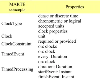
MARTE is a response to the OMG RFP to provide a UML profile for real-time and embedded systems [15]. MARTE is a successor of SPT, aligned on UML 2, and with a wider scope. MARTE introduces a number of new concepts, including time concepts, which are central to this paper. The main MARTE extensions of UML for time-related concepts are gathered in Table 1 and informally described below. A detailed description of the MARTE’s Time model is available in a research report [16], and will be soon published on the www.promarte.org site along with the full MARTE specification. In this paper, we focus on the concepts (domain view) rather than the formal UML specifi-cation of the profile (UML view).
The underlying model of time is a set of time bases. A time base is an ordered set of instants. Instants from different time bases can be bound by relationships (coincidence or precedence), so that time bases are not fully independent and instants are partially ordered. This partial ordering of instants characterizes the time structure of the application. This model of time is sufficient to check the logical
correctness of the application. Quantitative information can be added to this structure when quantitative analyses become necessary. Note that a specification of a temporal behavior may refer to points of time (instants) or to segments of time (durations). In the MARTE metamodel of time, Instant and
Duration are two distinct concepts, specialization of the
abstract concept of Time.
TABLE I. MAIN MARTE TIME CONCEPTS MARTE
concepts Properties
ClockType
dense or discrete time chronometric or logical accepted units
clock properties Clock unit ClockConstraint required or provided on: clocks TimedEvent on: clock every: Duration TimedProcessing
on: clock
duration: Duration startEvent: Instant finishEvent: Instant
The users of MARTE have access to the time structure through clocks. Here, clocks are not physical devices; they are model elements representing a general concept of time. While in SPT, clocks were implicitly bound to the physical time, in MARTE, a clock can be bound to any recurrent event. Thus, MARTE distinguishes two kinds of clocks: the
chronometric clocks, which make reference to physical time,
and the logical clocks, which focus on the ordering of instants, possibly ignoring the physical duration between instants.
Multiform time is defined and used in reactive
synchro-nous languages [6], [7]. It considers that flows (of event occurrences) are measured with different time units. At the design level, we know that actions take different amounts of time, but we don’t know yet how much each one would take [18]. Usually, time units are bound to physical time, but this is not necessary as illustrated below, where angular degrees are used as time units for crankshaft revolutions.
ClockType (Table 1) is a special class that specifies the
nature (dense or discrete) and the kind (chronometric or logical) of the represented time, a set of clock properties (e.g., resolution, maximal value…), and a set of accepted time units. For the chronometric clock types, time units are the usual time units: the second (s) and its derived units. Most logical clock types use a generic time unit called tick. In some cases, they may use more specific units: a processor cycle, for instance, or even units for physical quantities, like in the illustrative example of this paper, where time is measured in angular degree (°). This license to choose (logical) time units is a direct consequence of our decision to model multiform time. A Clock (i.e., an instance of a
ClockType) is characterized by its unit and the values (real
numbers) given to its optional properties: resolution,
maximalValue, offset. resolution gives the granularity of the
clock; maximalValue is the value at which the clock will roll over; offset specifies the origin instant. All the values are given with the unit of the clock. A predefined Clock is provided in the TimeLibrary of MARTE: idealClk. This hypothetical clock reads the dense “physical time”. It is used as a reference clock for the (imperfect) chronometric clocks defined by the users of the profile. A ClockConstraint sets dependencies up between clocks.
The idea behind the MARTE time model is that time-related concepts (e.g., event occurrences and behavior executions) make explicit reference to one or several clocks, through the on property (Table 1), as illustrated below, on events and behaviors. In UML, an Event describes a set of possible occurrences; an occurrence may potentially trigger effects in the system. A TimeEvent is an Event that defines a point in time (instant) when the event occurs. The specification can be either absolute or relative to some other instant. A TimedEvent is a TimeEvent, where the instant specification explicitly refers to a clock. Moreover, if the event is recurrent, a repetition period (duration between two successive occurrences of the event) may be specified. In UML, a Behavior describes a set of possible executions; an execution is the performance of an algorithm according to a set of rules. MARTE associates a duration, an instant of start, an instant of termination with an execution, these times being read on a clock. A TimedProcessing is a Behavior or an
Action with explicit references to clocks.
Examples on the use of these concepts are given in the next section.
III. APPLICATION TO AN AUTOMOTIVE SYSTEM
This section presents an automotive application: an ignition control and the knock correction in the case of a 4-stroke engine.
A. Spark-ignition engine
In a 4-stroke engine, a cycle is characterized by four phases: Intake, Compression, Combustion and Exhaust. These phases are driven by the camshaft, the positions of which are measured in angle degree (°).
Since the spark plug needs a delay to produce a flame front in the combustion chamber, the electric spark must be generated before the theoretical ignition point (ITDC: Ignition Top Dead Center).
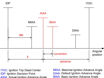
During the compression phase, at the Ignition Decision Point (IDP), an electronic control system determines the best angular position to generate an electric spark for igniting the compressed air-fuel mixture. The actual process is a bit more complex and involves remarkable points shown in Figure 1. The basic ignition advance angle (BIAA) is a function of the actual engine speed and the air/fuel ratio. Some corrections are then performed according to additional parameters leading to the actual ignition advance angle (AIAA). The angle from ITDC to AIAA is called the advance.
Figure 1. Ignition parameters
B. An example of correction: the knock
The knock is a physical phenomenon that generates an auto ignition during the combustion phase and leads to a lost of efficiency of the engine, a consumption increase, and may cause irreversible damage to the cylinder.
The knock control system detects and corrects this phenomenon. It consists of one or several noise sensors, and a controller, which performs the acquisition and computes the correction. Acquisition of the noise sensor signals is carried out during an observation window (KAW–Knock Acquisition Window). The starting point (KAWS–KAW Start) and the duration (KAWD–KAW Duration) of the window may vary. They depend on the knock intensity (KI) measured during the previous combustion phase. The knock controller is an adaptive system. A digital filtering is applied to the signal samples to deduce the knock intensity. This value is then used to adjust the advance (advance correction). More details about spark ignition engine management and knock control system can be found in an automotive handbook [17].
IV. MODELING BEHAVIOR WITH MULTIFORM TIME The ignition engine management is a typical example of real-time application gaining from a multiform time modeling.
A. Clock modeling and multiform time events
In a UML state machine, a label on a transition specifies a trigger that must reference an event. Labels like “after d” or “at i” implicitly defines a TimeEvent. The former specifies a relative instant, the later an absolute instant; these instants implicitly reference physical time. In MARTE, this convenient notation is extended to multiform time events, by applying the TimedEvent stereotype. In a 4-stroke engine, the succession of the phases is triggered by events associated with angular positions of the camshaft, not with physical time instants. In a multiform time approach, angular positions of the camshaft are considered as (logical) instants read on a logical clock: camClk. This clock represents a
discrete logical time, its unit is defined as °CAM (degree cam), its resolution is 0.5 (for instance), its offset is 0, and its
maximalValue is 360. All the values are implicitly given in
°CAM, the unit of the clock.
The events that trigger the transitions in the state machine shown in Figure 2 are stereotyped by TimedEvent, with the tag value on set to camClk. For instance, event IC (Intake closes) triggers the transition from Intake to Compression; it is a TimedEvent occurring 90 °CAM after entering state Intake.
Figure 2. State machine of a 4-stroke engine cycle
Note that in Figure 2, the whole state machine, which is a UML Behavior, has been stereotyped by TimedProcessing. The events involved in the state machine are, by default, bound to the same clock (i.e., camClk).
The 4StrokeEngineCycle state machine is a simplified specification of the behavior. In actual engine, the Intake and the Exhaust phases are overlapping. We specify this behavior using a UML interaction. Usually, interactions are shown as UML sequence diagrams. Instead, we use its variant called
timing diagram, introduced in UML 2.0. Identifiers on
vertical dashed lines are event identifiers. For clarity, we have highlighted them in red, but this is not normative. A timing diagram focuses on condition changing within and among life lines along a (horizontal) time axis. Of course, in MARTE this kind of diagram are extended to multiform time.
Figure 3. Timing diagram of a 4-stroke engine cycle for one cylinder Figure 3 describes the behavior of a 4-stroke engine. Instead of using the camClk, introduced above, we define a new logical clock: crkClk (crank clock), with °CRK (degree crank) for unit. This clock is bound to the rotation of the crankshaft. Since a full 4-stroke cycle needs two revolutions of the crankshaft, the maximal value of this clock is 720 °CRK. Its resolution is assumed to be 0.5 (for instance).
The camshaft and the crankshaft are mechanically bound: the latter runs twice faster than the former. Consequently, the two clocks camClk and crkClk are tighly dependent; this dependency is expressed by a ClockConstraint. Figure 4 shows the relationships between the instants of the two clocks. The ClockConstraint says that camClk is a subclock of crkClk, with instants of camClk being coincident with every second instants of crkClk. The concrete syntax for this
clock constraint is “camClk = crkClk filteredBy
0b(10)”, where 0b(10) is a periodic binary word [19]
standing for 1010…. (the infinite repetition of the 10 sequence). Note that having a logical clock does not prevent quantitative information: the instant value 0.5*(k-1) mod 720 °CRK is attached to the kth (k=1,2,…) instant of crkClk.
Figure 4. Clock constraint between camClk and crkClk
On the timing diagram in Figure 3, several events are named by acronyms explained in the lower part of the figure. For instance OTDC stands for Overlap Top Dead Center, which is the event occurring at the beginning of the cycle when the crankshaft is at its upper position. @tOTDC is a time observation of this event that denotes an instant (here the instant 0 on crkClk). The expressions written between curly braces are time constraints: they restrict the possible instants of occurrence of events. For instance, the occurrence of the
TimedEvent EC is constrained by { tOTDC + [5..20] }. This constraint means that on crkClk and with the values given in °CRK, tOTDC + 5≤ tEC ≤ tOTDC + 20.
B. Multiform time behavior
In real-time applications, the behavior executions are generally temporally constrained. A deadline imposed on the termination of an execution is a usual constraint that can be specified either by a duration (maximal execution time) or by an instant (occurrence of a timeout event). Here again, MARTE provides facilities to express such constraints on multiform time models. This is the object of this section.
act <<timedProcessing>> MICtrl
{ on = crkClk } AF RPM KI TableLookup BIAA Corrections KAW CIAA Adaptation ADV <<timedDurationConstraint>> { dMICtrl < m }
AF: Air/Fuel Ratio RPM: Engine speed ADV: Advance
KI: Knock Intensity KAW: Knock Acquisition Window
crkClk: crankshaft Clock MICtrl: Main Ignition Control
BIAA: Basic Ignition Advance Angle CIAA: Corrected Ignition Advance Angle
Figure 5: Ignition control for one cylinder (main part)
The activity diagram in Figure 5 specifies the behavior of the ignition control, at a high-level of description. The first action determines the basic ignition advance angle (BIAA) by a table lookup with two input parameters: the current air/fuel ratio and the current engine speed (i.e., the rotational speed of the crankshaft). The BIAA data is then used by the
Corrections action which takes into account various factors.
Only one, the knock intensity (KI), is shown in this study. The Corrections action yields two results: the corrected ignition advance angle (CIAA) and information on the knock acquisition window, described below. The last action generates the actual advance (ADV). This sequence of actions is triggered at the ignition decision point (IDP, already presented in Figure 1). The IDP event occurs at a fixed angular position, therefore at a fixed instant on the
crkClk. The new advance value must be available, under any
circumstances, before another angular event (MIAA– Maximal Ignition Advance Angle) which corresponds to the worst case (i.e., maximal engine speed and maximal allowed advance). Thus, the duration of the execution of the main ignition control activity must be less than angle δm of Figure 1. This multiform time duration constraint is written in a constraint compartment of the activity frame (Figure 5) and it references crkClk.
Figure 6. Ignition control for one cylinder
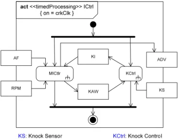
The main ignition control (MICtrl) activity is just a part of the ignition control (ICtrl) activity (Figure 6). The various corrections can be computed concurrently. For simplicity, we consider only the knock correction. The knock sensor is a vibration sensor that is sampled at 100 kHz (a classical frequency for vibration analysis). The use of a frequency unit makes implicit reference to physical time. In this application, as in many other control applications, logical clocks and chronometric clocks have to live together.
The activity diagram in Figure 7 represents the behavior of the knock control (KCtrl). The behavior is triggered by the occurrence of the ITDC event (i.e., when the crankshaft is at its top dead center at the end of the compression phase). This event occurs at a fixed instant (360 °CRK) on crkClk. The WaitWS action waits for the delay KAWS (Knock Acquisition Window Start, part of the KAW data). The knock signal acquisition action (KSA) is then carried out. The two events KWB and KWE denote the start and the end of this action. The acquisition fills in a buffer that is then read by the Filtering action. The knock intensity (KI) is the result of the filtering.
act <<timedProcessing>> KCtrl
{ on = crkClk }
KAW: Knock Acquisition Window KWB: Knock Window Begin
KWE: Knock Window End KSA: Knock Signal Acquisition WaitWS KAW KI KWB KSA KWE Filtering KS ITDC buffer
Figure 7. Activity diagram for the knock
The acquisition terminates either when the buffer is full or when the knock acquisition window duration (KAWD, part of the KAW data) has elapsed. The first occurring event causes the effective termination. This is a multiform time constraint. The latter condition is measured in °CRK while the former is bound to physical time through the imposed sampling period. This non standard time expression mixing different kinds of time, is typical of our multiform time approach. The constraint is specified by:
{ tKWE – tKWB = min ( sampleNb * Tsampling on idealClk, KAWD on crkClk) }, where sampleNb is the maximal number of samples in the buffer, Tsampling is the period of sampling (10 μs since the sampling frequency is 100 kHz),
idealClk is a predefined MARTE model element standing for
the ideal chronometric clock, KAWD is the knock acquisition window duration, a value given in °CRK and dynamically computed by the Corrections action (Figure 5). In order to evaluate this constraint, we have to know a clock constraint between idealClk and crkClk. This is detailed in the section on heterogeneous time constraint (Section V.B).
C. Usage
When considering an engine with four cylinders instead of a single cylinder, constraints become stronger. The ignition control activity (ICtrl) represented on Figure 6 must be executed for each cylinder. However, each cylinder has its own clock: crkClk1, crkClk2, crkClk3 and crkClk4. The clock becomes a parameter of the activity. Furthermore, each one of these clocks is very similar to each others. The commonalities amongst these clocks are defined by the
ClockType CRKClock; each cylinder clock becoming an
instance of CRKClock. The offset of each clock is different and determined by the engine firing sequence (order of combustion). For an engine whose firing sequence is 1, 3, 4, 2, the offsets of the clocks are respectively 0, 180, 540 and 360 for crkClk1, crkClk2, crkClk3 and crkClk4.
The dependencies are not limited to a simple sequencing of activities, we must also take into account hardware resources involved. The next section addresses this issue.
V. TIMING ANALYSIS
Section IV has introduced three clocks: camClk, crkClk and idealClk, and their dependencies expressed using constraints. Section V demonstrates the kind of analysis that can be performed on such constraints. We distinguish two kind of analysis. Analysis involving only one clock— homogeneous time constraints—and analysis involving several clocks—heterogeneous time constraints—. In the latter case, most of the time the constraints cannot be resolved.
A. Homogeneous time constraints
Each cylinder has its own storage for the knock intensity (KI), so there is no additional constraint coming from there. However, the buffer is shared by all cylinders. That means the filtering operation for one cylinder must complete before the start of the acquisition for the next firing cylinder. Looking at the specifications of the system, it is stated that
the knock acquisition window will begin before 55°CRK (KAWS) and that it will last 55°CRK (KAWD) at most. In the worst case, the whole operation will complete in under 110°CRK. With a four-cylinder engine, each cylinder has 180°CRK at most to complete (720°CRK divided by 4), which leaves us with 70°CRK more than required.
If we consider now the case of a six-cylinder engine each cylinder has 120°CRK at most to complete the computation (720°CRK divided by 6), which still leaves us 10°CRK more than required.
Finally, if we consider the case of a eight-cylinder engine, we only have 90°CRK to complete the computation (720°CRK divided by 8), which is not enough in the worst case (when the engine is running at its highest rotational speed). In this case, one solution may be to use two buffers in alternance. One of them is used to store samples about the cylinder currently in the combustion phase while the other one is used to process corrections for the previous cylinder.
B. Heterogeneous time constraints 1) Mono cylinder case
For an engine the maximal speed of which is 4500 rpm (revolutions per minute), since a revolution is 360 °CRK, the maximal engine speed is (4500/60)*360 = 27000 °CRK/s, so that 1°CRK ≥ 37 μs. This inequality is a constraint between the two clocks idealClk and crkClk.
Constraint on idealClk and crkClk: 1°CRK ≥ 37 μs
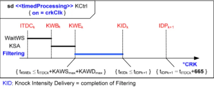
There are also constraints induced by the data flow specified in the activities. For instance, in the knock control activity, the buffer is a critical resource written by KSA, and read by Filtering. The timing diagram (Figure 8) shows that the filtering in cycle k has to deliver the knock intensity before the occurrence of the ignition decision point of the next cycle (IDPk+1 defined in Figure 1). IDPk+1 is at a fixed angular position (e.g., 665 °CRK after the ITDCk or equivalently 55 °CRK before the ITDCk+1). Given the maximal values of the knock acquisition window start (KAWSmax) and the knock acquisition window duration (KAWDmax), we deduce that
Filtering.duration ≤ 665 – KAWSmax – KAWDmax With the realistic values KAWSmax = KAWDmax = 55 °CRK, we get Filtering.duration ≤ 555 °CRK, which corresponds to 20.535 ms at the maximal engine speed. This constraint is easily satisfied by a microcontroller implementing the Filtering action.
2) Multi cylinder case
As shown in the homogeneous time constraints subsection, when several cylinders are considered, the duration constraints may become much more stringent. For instance, with a 4-cylinder engine, Figure 8 has to be modified, leading to Figure 9.
Figure 8. Knock acquisition and filtering timing diagram
The events (ITDC, KWB…) are now indexed by the cylinder number; ITDCm, KWBm, KWEm and KIDm refer to cylinder m, while ITDCn refers to cylinder n, the successor of m in the firing sequence. Note that the deadline for the KID is no longer IDP, but ITDCn. Instead of a duration of 665 °CRK between ITDCk and IDPk+1, we have a duration of 720/4 = 180 °CRK between ITDCm and ITDCn, which leaves us with 180 – 110 = 70 °CRK for the filtering duration in a 4-cylinder engine. Thus, at the maximal engine speed, the filtering duration should not exceed 70*37 = 2590 μs, much less than in the case of a single cylinder.
Figure 9. Knock acquisition and filtering timing-multiple cylinder case VI. CONCLUSION
We believe that multiform time is of first importance to specify constraints in real time embedded systems. In this paper, we have presented concepts essential to take into account this notion of multiform time.
UML is more and more present in the industry to bridge the gap between the domain experts, the customers and the developers. We have used UML to describe an example borrowed from the automotive domain and we have shown that with minor syntactic additions we can capture enough information so as to perform multiform-time analysis. We have partially validated requirements on the ignition control system. Some are related to performance and cost requirements (processor speed, number of buffers and their size); others are variability requirements (number of cylinders). The studied example is mainly control-dominated without considering timed communications, which are of major concern in automotive applications. This issue has to be addressed in the future.
The MARTE Time model is not restricted to the automotive application domain. It has been defined for the specification of time aspects in real-time embedded systems at large. We have tried to keep syntactical changes as small as possible to be able to reuse existing models, to preserve
legacy and so as the business domain is not altered too much. However, the semantic shift is quite important since the notation can address a very large family of problems where time becomes a first class citizen.
ACKNOWLEDGMENT
This study has been partially supported by the RNTL Memvatex project [20], which provides the application case study, and the project Usine Logicielle, sub-project OpenDevFactory [21], which supports the implementation of the MARTE Time profile.
The original publication is available at ieee.org (http://dx.doi.org/10.1109/SIES.2007.4297340).
REFERENCES
[1] F. A. Schreiber, “Is Time a Real Time? An Overview of Time Ontology in Informatics”, in W. A. Halang, A. D. Stoyenko (Eds.) Real Time Computing, Springer Verlag NATO-ASI, vol. F127, 1994, pp.283-307.
[2] D. G. Messerschmitt, “Synchronization in Digital System Design”, IEEE Journal on Selected Areas in Communications, vol. 8, no 8, october, 1990, pp.1404-1419.
[3] L. Lamport, “Time, Clocks, and the Ordering of Events in a Distributed System”, Communications of the ACM 21, (7), 558-565, 1978. [4] R. Schwarz and F. Mattern, “Detecting Causal Relationships in Distributed Computations—in Search of the Holy Grail”, Distributed Computing 7, 149-174, 1994.
[5] OMG, Enhanced View of Time Specification, version 1.2, formal/04-10-04, October 2004.
[6] A. Benveniste, G. Berry, “The Synchronous Approach to Reactive and Real-Time Systems”, Proceedings of the IEEE, vol 79, no 9, September, 1991, pp.1270-1282.
[7] A. Benveniste, P. Caspi, S. A. Edwards, N. Halbwachs, P. Le Guernic, R. de Simone, “The Synchronous Languages 12 Years Later”, Proceedings of the IEEE, vol 91, no 1, January, 2003, pp.64-83.
[8] OMG, Unified Modeling Language: Superstructure, version 2.1, ptc/2006-04-02, April 2006.
[9] B. Selic. “On the Semantic Foundations of Standard UML 2.0”, SFM-RT 2004, LNCS 3185, Springer-Verlag, pp. 181-199, 2004.
[10] OMG, UML Profile for Schedulability, Performance, and Time Specification, version 1.1, formal/05-01-02, January 2005.
[11] OMG, Systems Modeling Language (SysML) Specification, ad/2006-03-01, April 2006.
[12] EAST-ADL: The EAST-EEA Architecture Description Language, ITEA Project Version 1.02, 30.06.2004, www.east-eea.net
[13] S. Graf, I. Ober, I. Ober: “A real-time profile for UML”, STTT, Int. Journal on Software Tools for Technology Transfer, Springer-Verlag, vol 8, no 2, April 2006, pp. 113-127.
[14] L. Apvrille, P. de Saqui-Sannes, F. Khendek: “TURTLE-P: a UML profile for the formal validation of critical and distributed systems”, Softw Syst Model, Springer-Verlag, vol 5, 2006, pp. 449-466.
[15] OMG, UML profile for Modeling and Analysis of Real-Time and Embedded systems (MARTE), Request for proposals, realtime/2005-02-06, February 2005.
[16] C. André, F. Mallet, R. de Simone, “Modeling Time(s) in UML”, I3S Research Report, RR-2007-16-FR, (23 pages), May 2007.
[17] Bosch Automotive handbook, 6th Edtion, Bentley Publishers, ISBN
0-8376-1243-8, October 2004.
[18] A. Benveniste, C. Jard, S. Gaubert, “Algebraic Techniques for Timed Systems”, Proceedings of the 9th Intern. Conf. on Concurrency Theory,
LNCS, vol 1466, pp 373-388, 1998.
[19] A. Cohen, M. Duranton, C. Eisenbeis, C. Pagetti, B. Plateau, M. Pouzet, “N-Synchronous Kahn Networks - A Relaxed Model of Synchrony for Real-Time Systems”, ACM Intern. Conf. On Principles of Programming Languages, Charleston (SC), January, 2006.
[20] RNTL project MEMVATEX, www.memvatex.org
[21] Projet Usine Logicielle, pôle SYSTEM@TIC PARIS REGION,