HAL Id: hal-01259243
https://hal.inria.fr/hal-01259243
Submitted on 20 Jan 2016
HAL is a multi-disciplinary open access
archive for the deposit and dissemination of
sci-entific research documents, whether they are
pub-lished or not. The documents may come from
teaching and research institutions in France or
abroad, or from public or private research centers.
L’archive ouverte pluridisciplinaire HAL, est
destinée au dépôt et à la diffusion de documents
scientifiques de niveau recherche, publiés ou non,
émanant des établissements d’enseignement et de
recherche français ou étrangers, des laboratoires
publics ou privés.
suspended cable-driven parallel robots
Jean-Pierre Merlet
To cite this version:
Jean-Pierre Merlet. On the real-time calculation of the forward kinematics of suspended cable-driven
parallel robots. 14th IFToMM World Congress on the Theory of Machines and Mechanisms, Oct 2015,
Taipei, Taiwan. �hal-01259243�
On the real-time calculation of the forward kinematics of suspended cable-driven
parallel robots
J-P. Merlet∗
INRIA
Sophia-Antipolis, France
Abstract— This paper addresses the problem of the for-ward kinematics of cable-driven parallel robots (CDPR) having elastic or non elastic cables under the assumption that the cables are submitted to small changes in their lengths compared to an initial situation at which the pose is known, a situation that is typical of a real-time forward kinematics used for control purposes. We show that at the initial point it is necessary to have not only the pose but also thecable configuration, i.e. having the knowledge of which cables are under tension and that the result of the forward kinematics should be both the pose and the cable configu-ration after the change in cable lengths. We exhibit a first algorithm that allows one to determine all possible final poses and cable configurations. Then a second algorithm is proposed to determine all possible cable configurations also during the coiling process which is an important point as the CDPR state, including the cable tensions, may dras-tically change at this point. The last algorithm assumes a model of the coiling process and is able to determine the unique final pose and cable configuration. These al-gorithms provide safer real-time forward kinematics which will improve the CDPR control
Keywords: clear, cable-driven parallel robots,forward kinemat-ics,cable configurations, real-time
I. Introduction
Cable-driven parallel robot (CDPR) are robots whose platform are connected to the ground by a set of cables that can be uncoiled or coiled. The study of CDPR has started about 30 years ago with the pioneering work of Albus [1] and Landsberger [2] but there has been recently a renewed interest in such a robot, both from a theoretical and applica-tion viewpoint. The kinematics analysis of CDPR is much more complex than the one of parallel robot with rigid legs as static equilibrium has to be taken into account [3], [4], [5], [6] and is still an open issue especially as not all ca-bles of a robot with m caca-bles may be under tension [7], [8], [9], [10], [11] and that only stable solutions have to be de-termined [12]. Numerous applications of CDPRs have been mentioned e.g. large scale maintenance studied in the Euro-pean project Cablebot [13], rescue robots [14], [15], large telescope [16], rehabilitation [17], [18] and transfer robot for elderly people [19] to name a few.
∗Jean-Pierre.Merlet@inria.fr
The proprioceptive measurement on such a robot is usu-ally the cable lengths as other physical quantities such as orientation of the cables or their tensions are difficult to measure. The kinematic analysis of such robot is drastically influenced by the cable model that is used. For example a cable may be supposed mass-less and non elastic, mass-less but elastic or deformable and elastic. In this paper we con-sider only mass-less cables and a specific class of CDPR: suspended CDPR. In this class there is no cable that can exert a downward force that is larger than its own weight (figure 1).
Before going on we will introduce some notation. The output point of the coiling mechanism for cable i will be de-noted Aiwhile this cable is attached at point Bion the
plat-form. We define an absolute frame(O, x, y, z) and we as-sume that the coordinates of Aiin this frame are known. In
the same manner we define a mobile frame(C, xr,yr,zr)
that is attached to the platform (figure 1). Without lack of generality C will be assumed to be the center of mass of the platform with coordinates(xc, yc, zc). We assume that
the coordinates of Biin the mobile frame are known. Our A1 A2 A3 A4 A5 A6 A7 B7 B3 B1 B2 B4 B5 B6 C ρ2 z y x Fig. 1. A suspended CDPR
cable model assume that the cable profile is directed along the line going through the points A, B as soon as the cable is under tension. For non elastic cables the length of a ca-ble will be denoted ρ while for elastic caca-ble ρ will denote its real length while l0will denote its length at rest.
A major problem with CDPR is that they have usually several solutions to the forward kinematic (FK) problem
(i.e. being given the cable lengths determine the pose of the platform). This is usually the case for parallel robots but the situation is even worse for CDPR and is still yet not fully understood. A major point is that each solution of the FK leads to a specific set of cable tensions together to a specific pose. As determining the pose and the tensions are key factors for safety and control it is essential to be able to determine the current state of the robot. This problem may stated as follows: being given a state of the robot(ρ, X) for non elastic cables or(l0,X) for elastic cables, where X
de-notes the pose of the platform, determine the poseX1of the
robot when the components of ρ (l0) are changed to ρ+∆ρ
(l0+ ∆l0), where∆ρ(l0) is a vector of ”small” amount
of changes in the cable lengths that occurs after a ”small” amount of time∆t. This is typically the problem we have to solve for the real-time calculation of the FK: after the calculation of the current pose based on the cable lengths measurement a control law will calculate a command for the actuators that will not be changed during the sampling time of the controller (we do not consider here other con-trol schemes that do not use the measurements of the cable lengths, for example the one using the visual observation of the direction of the cables [20]).
For robot with rigid legs we have exhibited an algorithm that first check if ∆ρ is small enough so that there is an uniqueX1that can be reached starting fromX and if this
is the case is able to computeX1with an arbitrary
accu-racy [21].
Unfortunately we will see that such scheme will not work for CDPR. But first we may summarize the known result about the FK of CDPR as follow:
• for mass-less and not elastic cables (case 1) for a CDPR
with m cables the FK always amounts to solve a set of square systems of equations. Indeed we cannot assume that in the current pose all m cables are under tension and to find all FK solutions we have to consider all possible com-binations of cables under tension. Note that if m >6 there cannot be more than 6 cables under tension simultaneously. Still for a given number of cables the minimal FK equa-tions will be square with 6 equaequa-tions for 6 cables and m+ 6 for m < 6 cables (6 parameters for the pose and m cable tensions). But even with this complexity all the solutions found by solving the different sets of equations may not all be valid. Indeed for a given solutionXs we have to
ex-amine first the tensions of the cables that must all be pos-itive. Then we have to consider the lengths of the cables that are supposed to be slack: for each of them this length must be greater than the distance between the A, B points for the poseXs. Hence this differs from the FK of parallel
robots with rigid legs where a single square system has to be solved and all solutions are valid.
• for mass-less but linearly elastic cables (case 2) all cables
may be under tension even if m >6 but it may also happen that we have slack cables. The tension τ in the cable is written as τ = k(ρ − l0) where k is the linear stiffness, ρ is
the real length of the cable and l0its length at rest that are
supposed to be known. Hence the minimal FK has m+ 6 unknowns (6 parameters for the pose and mρ) and m+ 6 equations (6 from the statics equilibrium and m equations that state that the distance between A, B should be ρ). Still one or more of the cables may be slack (i.e. ρ < l0) and
as in case 1 we have thus to consider all combinations of cables under tension
• for deformable and elastic cables (case 3) the FK amounts
to solve a single square system of equations that has usually several solutions [22].
In case 3 the algorithm presented in [21] may be applied to solve the real-time FK but cannot for case 1 and 2. Indeed atX we know which cables are under tension and which one are slack (if any). Unfortunately atX1 the set of
ca-bles under tension may be different from the one atX and therefore the system of equations of whichX1is a solution
is different from the one atX.
This paper addresses the following topics for CDPR in case 1 and 2:
• determine if a change (or more than one) in the set of
cables under tension may occur when changing the cable lengths by∆ρ(l0)
• if yes determine the new set(s) of cable under tension • determine the poseX1
II. Solving the real-time FK A. The statics equations
A suspended CDPR is usually submitted only to gravity (and possibly to small disturbances that we will neglect). The wrench applied on the platform will be denotedF and the equations relating this wrench to the tension τ in the cables are:
F = J−Tτ (1)
whereJ−T is the6 × m jacobian matrix (where m is the
number of cable under tension) whose i-th column is
((AiBi ρi
CBi∧ AiBi
ρi
))
B. The cable configuration concept
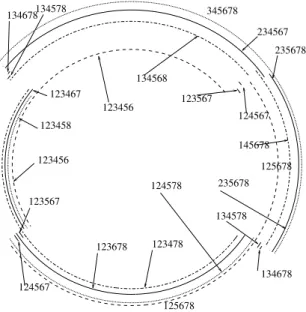
A cable will be denoted dominant if it exerts an force on the platform and non dominant if it is slack. A cables configuration(CC) for a CDPR with m cables is a set of m booleans whose i-th member is set to 1 if the i-th cable is dominant and set to 0 otherwise. This concept is quite important because at a given pose the CDPR may have dif-ferent cable configurations. For example we have consid-ered a specific robot with 8 cables that has to move along an horizontal circle while keeping constant the orientation of its platform. Figure 2 shows the circular arcs for which the various CC with 6 cables are valid (the arcs have been offsetted to make them visible). It may be noticed that this trajectory cannot be fully completed with the same CC and
123456 123456 123458 123467 123478 123567 123567 123678 124567 124567 124578 125678 125678 134568 134578 134578 134678 134678 145678 234567 235678 345678 235678
Fig. 2. The possible CC on a circular trajectory. The arc have the same radius but have been enlarged in order to show the different CC
that there may be up to 4 different CC’s for a pose. The cable configuration allow to determine what are the cable tensions (which differ from one CC to another one) but also the performances of the CDPR at this pose. For example it is well known that an error∆ρ on the cable lengths ρ leads to an error in the platform positioning∆X such that
∆X = J∆ρ
AsJ is dependent upon the CC so will be the positioning accuracy.
C. First algorithm
This algorithm will simply try to determine all the valid CC to which may lead the change from ρ to ρ+ ∆ρ i.e. to solve the FK for each CC. For non elastic cables and a CDPR with a total of m cables, n of which are under tension we have the following equations and inequalities under the assumption that the numbering of the cables is such that the cables from 1 to n are under tension:
||AiBi||2= (ρi+ ∆ρi)2i∈ [1, n] (2)
||AiBi||2− (ρi+ ∆ρi)2≤ 0 i ∈ [n + 1, m] (3)
τ= {τ1, . . . , τn} τi>0 ∀i ∈ [1, n]
F = J−Tτ (4)
the statics equations being used in the FK solving only if n < 6 (if n = 6 only the equations (2) are used and the statics equations are used only a posteriori to eliminate so-lutions leading to at least one negative τi). To model the
pose of the platform we use a parametrization that depends upon the number n:
• if 4 ≥ n ≤ 6: we use as parameters the coordinates
of 4 of the B says the coordinates ofOB1, . . . ,OB4that
are called the reference points. It follows that we have ∀j > 4 OBj=Pm=4m=1αmOBmwhere the αmare known
constants. At the poseX the coordinates of the reference points Bs
j are known.
• if n = 3: we choose B1, B2, B3 as references points
and we have∀m > 3 B1Bm = β1B1B2 + β2B1B3 +
β3(B1B2 × B1B3) where the β are known constants. • if n = 2: C, B1, B2 all lie in the same vertical plane
that includes A1, A2and the location of C may be deduced
from the location of B1, B2with 2 possible solutions (one
below the line B1B2, one over it). Hence we choose the
coordinates of B1, B2as unknowns
• if n= 1: A1, B1, C lie on the same vertical line with C
having two possible locations (over or below B1). The z
coordinates of B1is chosen as unknown
The motivation for using this parametrization will be ex-plained later on. We will not consider the case n ≤ 2 that can be trivially solved. Now let us look at the equation
F = J−Tτ τ = {τ
1, . . . , τn}
that is used for the FK solving if n <6 with the components of τ as unknowns. At the opposite of the pose parameters there is no a-priori rules that allows one to establish bounds for the elements of τ . However we may extract from these equations a linear system in τ of size n× n. After solv-ing this system we may report the result in the remainsolv-ing 6 − n equations. Hence we always end up with a system constituted of:
• n equations from the linear system
• 6 equations (n from (2) plus6 − n remaining after the
solving of the linear system)
• m− n inequalities (3)
In terms of unknowns we have
• the pose parameters (12 if4 ≥ n ≤ 6, 9 if n = 3) • the n elements of τ
As we may see we have always more unknowns than equa-tions. However the parametrization always allow us to end up with a square system by adding equations stating that the distance between the reference points Bi, Bj is a known
constant. We will no more mention this additional equa-tions in the remaining of the paper but they are required to get a square FK system.
For elastic cables the change in cable lengths affect l0
which will become l0+ ∆l0. The equations are:
||AiBi||2= ρ2i (5)
F = J−Tτ τ = {k(ρ
i− li0− ∆l0i)} (6)
which are valid for all i∈ [1, n]. We have also the inequal-ities
l0i + ∆l0i − ρi≤ 0 ∀i ∈ [1, n] (7)
||AiBi||2− l0i − ∆l0i ≤ 0 ∀i ∈ [n + 1, m] (8)
but here we have to consider all combination with n≤ m. In terms of unknowns we have
• the pose parameters (12 if4 ≥ n ≤ m, 9 if n = 3) • the ρiwith i∈ [1, n]
For this first algorithm we will assume that we may bound the pose parameters e.g. by assigning a maximal velocity to the platform from which we will deduce a carte-sian box that will include the final position of the reference points. Under that assumption we have bounded variables (the pose parameters) and unbounded unknowns (the τifor
the non elastic case and the ρi for the elastic case). The
presence of bounded variables lead us to propose an interval analysis solving method (that requests bounded unknowns) and we will see later on that the presence of unbounded un-knowns is not a problem, We will now describe our generic FK solving method.
C.1 Solving with interval analysis
Interval analysis allows to calculate exactly (i.e. with an arbitrary accuracy) all solutions of a system of equations that lie within a bounded region, called the search space. Without going into the details (that may be found in [23], [24], [25], [26]) the solving principle is first based on the interval evaluationof the equations: being given intervals for the unknownsW (which define a box in the unknowns space) and a function of these unknowns f(W) the inter-val einter-valuation of f is an interinter-val[U, V ] that is guaranteed to satisfy that for all vectorsW whose components all lie in the corresponding intervals we have U ≤ f (W) ≤ V . There are several methods for computing such an interval evaluation, all having the drawback that U may be un-derestimated (i.e. the minimum of f over the intervals is larger than U ) and/or V may be overestimated (i.e. the maximum of f over the intervals is larger than V ). How-ever the differences between U, V and the minimum, max-imum decrease with the size of the input intervals. Such an overestimation occurs when there are several occurrences of the same variable in f . A typical example of overes-timation is to consider f = x − x when x ∈ [−1, 1] as f([−1, 1]) = [−1, 1] − [−1, 1] = [−2, 2] that indeed in-clude the solution 0 but with a large overestimation.
Clearly if U > 0 or V < 0, then f cannot cancel for any point in the box. The second component of an inter-val analysis algorithm is the branch and bound scheme. In this scheme we have a listL of box(es) which has, at the start of the algorithm, a single element, the search space and an index i initialized to 1. The algorithm look at the i-th box in the list and calculate the interval evaluation of each equation of the system for this box. If for each of these evaluations we have U < 0 and V > 0, then we bi-sect the box in two by selecting one of the unknowns and splitting its current interval at the mid-point. This process creates two new boxes that are stored at the end ofL and the index i is incremented. If U > 0 or V < 0 then the index i is incremented. After each bisection the size of the box decreases so that we may use the third tool of interval analysis which is the Kantorovitch theorem. It states that if
some conditions, that may be calculated with interval anal-ysis, are fulfilled, then the box includes a single solution of the system and that this solution may be obtained by using the Newton-Raphson scheme with as initial guess the cen-ter of the box (see section V). If this theorem is fulfilled for a given box we have determined a solution of the system and the index i is incremented. The algorithm completes when the index i is larger than the number of elements in L. Such an algorithm cannot miss a solution and will usu-ally provide all the solutions in the search space unless the numerical accuracy is not high enough (in this case it is nec-essary to extend the floating point arithmetic and numerous packages allow to do it).
This principle may be extended to deal with inequality. For example if the problem is to check if f(W) ≤ 0 a box will be deleted from the listL if U > 0 and the inequalities will always be satisfied for any point of the box if V ≤ 0.
For non elastic cables an objection to the use of interval analysis for n < 6 is that we don’t have bounds for the components of τ . However they are not necessary. Indeed let us consider the linear system extracted from the statics equations. As the matrix J−T is pose dependent and as
the pose parameters are intervals we have a so-called linear interval system. Interval analysis allows one to solve such system i.e. provide ranges for the components of τ that in-clude all the solutions of all scalar linear system inin-cluded in the linear interval system. Without going into the details this solving may fail for a given box especially because the linear interval system includes one or several singular sys-tem, in which case the box will be bisected and as we may assume that the robot is not in a singular pose a sufficient number of bisections will always guarantee that the interval linear system may be solved.
For elastic cables we will distinguish two cases:
• n ≤ 6: we use the interval solving for the linear
sys-tem that may be extracted from (6) to bound the unknowns ρi together with the interval evaluation of (5) that provide
another mean to evaluate these bounds
• n >6: we use the interval evaluation of (5) to determine
bounds for the ρi
C.2 Solving the FK
As seen previously the unknowns of our FK problems are just the pose parameters whose intervals are described by a box. We now describe the processing of a given box of the listL for non elastic cables:
1. if n <6
(a) solve the linear interval system (b) if the solving fails bisect the box
(c) if one component of τ has a negative upper bound moves to the next box in the list
2. interval evaluation of the 6 equations (2) and the one re-maining from (1). If one of this evaluation has a strictly negative upper bound or a strictly positive lower bound moves to the next box in the list
3. apply Kantorovitch theorem withX0being the center of
the box:
(a) if this test succeed calculate the solution and substitute the box by this solution
4. interval evaluation of the inequalities (3) for the non dominant cable(s)
(a) if the lower bound of one evaluation is strictly positive moves to the next box in the list
5. if the box has been reduced to a solution, then store the solution and moves to the next box in the list
6. bisect the box
For elastic cables the processing of a given box of the listL is:
1. if n≤ 6
(a) solve the linear interval system in ρiderived from (6)
(b) if the solving fails bisect the box
(c) if the upper bound of one ρi is lower than l0i + ∆l0i
moves to the next box in the list
(d) interval evaluation of the equations (5) and of the m− n remaining equations of (6). If one of this evaluation has a strictly negative upper bound or a strictly positive lower bound moves to the next box in the list
2. if n > 6 determine bounds for the ρi by the interval
evaluation of (5)
(a) if the upper bound of one ρi is lower than l0i + ∆l0i
moves to the next box in the list
(b) if the lower bound of one ρiis lower than l0i+ ∆l0i set
this bound to li0+ ∆li0
(c) interval evaluation of the 6 equations (6). If one of this evaluation has a strictly negative upper bound or a strictly positive lower bound moves to the next box in the list 3. apply Kantorovitch theorem on the full system withX0
being the center of the box:
(a) if this test succeeds calculate the solution and substi-tute the box by this solution
4. interval evaluation of the inequalities (7, 8)
(a) if the lower bound of one evaluation is strictly positive moves to the next box in the list
5. if the box has been reduced to a solution, then store the solution and moves to the next box in the list
6. bisect the box
Note that if n >6 we may possible refine the interval for the ρi. Indeed (6) may be seen as a linear system in 6
ar-bitrary ρi. The solving of this system will provide bounds
for these ρithat may used to refine the bounds determined
by using (5). The specific parametrization of the platform pose that we have used may be explained here. Indeed all the equations involved in the FK are algebraic and of second order in terms of the unknowns. This implies that the Hes-sian matrix of the system will be a constant matrix whose norm can thus be computed beforehand. As this norm is used in the Kantorovich theorem having a constant norm allows one to speed up the Kantorovitch test.
Using this process we are able to find all the solutions of all FK problems under the assumption that there is no
dras-tic change in the pose of the parameters during the coiling. If there is a single solution we may have determined the pose of the platform together with its CC after the change in the cable lengths. If we have multiple solutions we can-not determine the current pose and CC.
We will now describe a safe real-time FK method that takes into account possible CC change during the coiling process.
D. Second algorithm
In our previous algorithm we have assumed no drastic change in the platform pose. But unfortunately this as-sumption may not always hold. For example figure 3 shows changes of CC for infinitesimal changes of cable lengths that leads to a significant change in the platform pose. On the first image the robot has 6 cables under tension and its pose correspond to one solution of its FK. On the second image the CDPR moves suddenly to a CC with 4 cables un-der tension but one which is mechanically unstable which explain why (third image) it moves to a new pose with 6 ca-bles under tension but on another kinematic branch of the FK than the one from which it started, thereby exhibiting a very different orientation.
Such situation cannot be detected with our first algorithm and requires to consider not only the final cable lengths but how these lengths change with respect to time. We will now consider the CC under the assumption that the cables lengths may have any value in their ranges[ρ, ρ + ∆ρ] for non elastic cables or that their lengths at rest may have any value in[l0, l0+ ∆l0] for elastic cables. Our purpose will
be to determine what are the possible CC of the CDPR un-der that assumption. We still use the assumption that the pose of the platform may be bounded and we will check what are the possible CC in the neighborhood ofX. As the motion of the platform are continuous we will look at spe-cific time at which the initial CC may co-exist with another CC. For non elastic cables such a situation may occur if 1. the tension in a dominant cable (or in several cables) part of the initial CC goes to 0
2. the length of a non dominant cable (or of several cables) not part of the initial CC becomes exactly the distance be-tween the A, B
For elastic cables the situation may occur if
1. the real length ρ of one (or several) cable is exactly its length at rest
We will assume that the initial CC is such that 6 cables are under tension for non elastic cables and that all cables are under tension for elastic cables. We consider the full scale FK equations of the CDPR i.e. equations (2, 4) for non elas-tic cables and (5, 6) for elaselas-tic cables. For fixed values of ρ or l0we have a square system of equations but here we as-sume that ρ, l0may have interval values i.e. that these
con-straints describe a family of square systems of equations. Note however that the Kantorovitch theorem (section V)
Fig. 3. An experiment showing changes of cable configuration for an infinitesimal change in the cable lengths leading to very different poses
may still be used. Indeed in spite of ρ, l0having interval values:
• the Jacobian matrix of the system atX0 is still a scalar
matrix
• F(X0) will have now interval values, leading to intervals
forΓ0F(X0) but whose norm will still be bounded
In consequence the interval values of ρ, l0will prohibit us
to calculate the solutions but if the Kantorovitch conditions are fulfilled, then we are sure that there will be a single solution for any system in the family.
We will now consider separately the non elastic and elas-tic cables cases.
D.1 Non elastic cables
We will consider as unknowns the pose parameters, the ρ and the τ of the dominant cables and hence all the un-knowns are bounded (the bounds for the τ being obtained with the method described in the first algorithm).
We will consider in sequence all combinations of cases where
1. one or several cables is (are) such that τj = 0
2. the length of a cable (or of several cables) not part of the initial CC becomes exactly the distance between the A, B 3. the length of a cable (or of several cables) part of the ini-tial CC becomes larger than the distance between the A, B For the first case we will set k τj = 0 into equations (4) and
use as unknowns for an interval analysis algorithm the pose parameters, the ρ and the remaining components of τ but only the pose parameters and the ρ will be bisected. Note that as the ρ have interval values we have a family of square system of equations. The processing of a given box of the algorithm is as follows:
1. for all cables in the initial CC interval evaluate the equa-tion||AiBi||2− ρ2i. If one of the interval evaluation does
not include 0 move to the next box
2. interval evaluate (3) for the cable not part of the CC. If one of these inequality has a positive lower bound move to the next box
3. extract an interval linear system of size6 − k from (4) and solve it in the6 − k elements of τ :
• if the solving fails bisect the box and move to the next
box in the list
• if one of the τjhas a negative upper bound move to the
next box
4. plug the τ in the remaining k equations from (4), inter-val einter-valuate them and if one of the interinter-val einter-valuation does not include 0 move to the next box
5. if one of the τj has a negative lower bound then bisect
the box and move to the next box in the list 6. we check if the Kantorovitch conditions hold
• if no we bisect the box and move to the next box in the
list
• if yes we have determined that a new solution CC may
be reached by the CDPR
In the second and third case we will assume that any number k, with k ∈ [1, 6], of cables may be such that ||AiBi||2 = ρ2i. The full FK system will still be square.
We will use as unknowns for an interval analysis algorithm the pose parameters and the kρ.
For a given box we use the following steps:
1. for all k cables interval evaluate the equation||AiBi||2−
ρ2
i. If one of the interval evaluation does not include 0 move
to the next box
2. interval evaluate (3) for the m− k cables not part of the k cables. If one of these inequalities has a positive lower bound move to the next box
3. solve the interval linear system of size k extracted from (4) in the τ :
• if the solving fails we bisect the box and move to the
next box in the list
• if one of the τ has a negative upper bound, then move to
the next box
4. if k < 6 plug the τ in the remaining 6 − k equations from (4), interval evaluate them and if one of the interval evaluation does not include 0, then move to the next box
5. check if the Kantorovitch conditions hold
• if no we bisect the box and move to the next box in the
list
• if yes we have determined that a new solution CC may
be reached by the CDPR
If solution CC’s are found then there will be set of ρ’s for which the CDPR may be submitted to a change of CC.
D.2 Elastic cables
We will consider as unknowns the pose parameters, the components of ρ and the components ofl0
and hence all the unknowns are bounded (the bounds for the components of the ρ being obtained with the method described in the first algorithm).
We will consider in sequence all combinations of cases where one or several cables is (are) such that ρj = l0j and
use an interval analysis algorithm in each case after having removed from the equations (5,6) the equation(s) involving cable(s) j. As we remove as many equations as unknowns we still end up with a square system. For a given box of the algorithm:
• we interval evaluate the equations of the new system. If
one interval evaluation does not include 0 we move to the next box
• if for a cable k the upper bound of||AkBk|| is lower than
the lower bound of lk0, then we move to the next box
• we check if the Kantorovitch conditions hold
– if no we bisect the box
– if yes we have determined that a new CC may be reached by the CDPR
After completing the algorithm for all cases we will have determined all possible CC of the CDPR during the cable lengths change that are different from the initial CC. If there is no such CC then the initial CC will be kept during the ca-ble lengths changes and the possica-ble final pose(s) will be determined using the first algorithm. If more than one so-lution is found, then we cannot solve properly the FK prob-lem.
E. Real time FK with a coiling model
The first FK algorithm is just able to determine if a CC different from the initial one may be valid at the end of the cable motion and thus is not completely safe. The second FK algorithm will detect if a change of CC may occur dur-ing the cable motion and is therefore fully safe from the CC view point. However both algorithms are not fully safe for finding the pose at the end of the cable motion because they both assume small motion of the platform and still may provide not a single solution. Furthermore from the CC viewpoint the second algorithm is ”worst case”: although a change in CC may occur the real coiling process may be such that this change will not occur. To take into account the real coiling we will assume a model for this process.
E.1 Coiling model
A typical coiling model will provide the ρ or l0as
func-tions of time. Being given the stateS of the actuator at time t0the cable length at time t > t0will be obtained as:
ρ(t) = G(S, t) (9) For example assume that an electrical motor is used to turn the drum of a winch. If at time t0the velocity of the motor
is V0and a control law imposes a desired velocity Vc, then
the velocity of the motor is
V(t) = Vc+ (V0− Vc)e−
t−t0 U
where U is a known constant. If θ0is the rotation angle of
the motor at time t0, then the angle at time t is obtained as:
θ(t) = Vct− (V0− Vc) U e−
t−t0
U + (V 0 − Vc)U − Vct0+ θ0
If ρ0is the cable length at time t0, then the cable length at
time t will be:
ρ(t) = ρ0+ K(θ(t) − θ0)
where K is a constant that depends upon the reduction gear of the motor and the drum radius.
E.2 FK for non elastic cables
We will assume that at time t0the CDPR is in the initial
CC at poseX with cable lengths ρ0and that we are
inter-ested in determining the robot pose and CC at time t0+∆T .
If n is the number of cables under tension at time t0and if
we assume the CDPR will stay in the same CC the govern-ing equations of the system are:
||AiBi||2= ρi(t) i ∈ [1, n] (10)
||AiBi||2− ρi(t)2≤ 0 i ∈ [n + 1, m] (11)
τ = {τ1, . . . , τn} τi>0 ∀i ∈ [1, n]
F = J−Tτ (12)
Let us choose a time increment∆t < ∆T . The coiling model allows us to determine an interval value for each of the ρithat will include all possible values of ρifor any time
in the range[t0+ ∆t]. We then apply Kantorovitch
theo-rem on the 6 equations (10) if n = 6 or on the equations (10,12) if n <6. If the Kantorovitch conditions do no hold we divide∆t by 2 and repeat the process. If they hold we are able to calculate the robot pose at time t0+ ∆t together
with the cable tensions. If the cable tensions are all positive and the inequalities (11) are verified we have a new starting pose and we repeat the process from this point until the time reaches t0+ ∆T . But it may perfectly happen that in the
time interval[t0, t0+ ∆t] there is a time such one of the
in-equalities (11) are not satisfied or one of the cable tensions becomes negative. To determine if one such configuration exists we will consider the two following problems:
• for each cable j not in the CC find a time t1in[t0, t0+
∆t] such that equations (10) are verified together with ||AjBj||2 = ρj(t). For each j we add an equation and
the unknown t1 and therefore we have a square system of
equations. Interval analysis is used to solve this problem in t1
• for each cable j in the CC find a time t1in[t0, t0+ ∆t]
such that the solving of equations (12) leads to τj= 0. For
this purpose we set τj= 0 and we solve the system (10,12)
which is still square as we have removed the unknown τj
but have added the unknown t1.
Let define T = {t1
1, t21, . . . t p
1} be the set of times t1
or-dered by increasing value. At any of the time in this set two different CC coexist: the initial one CC0 and a new one
CC1. We consider each of the time t1in the set by
increas-ing value and consider the situation at time tj1+ ǫ where ǫ
is a small quantity such that tj1+ ǫ < tj+11 . At this time the CC of the CDPR may be either CC0 or CC1. In the
first case at time tj1CC0and CC1were equivalent but the
coiling moves the CDPR back to CC0. In the later case the
CDPR has moved to the new CC CC1: a cable
configura-tion change has occurred. We solve the FK system for both cable configurations and as the CDPR must be in an unique CC only one of the two FK systems has a valid solution (i.e. verifying the inequalities (11) and having positive τ ). If the valid CC is CC0 we move to the time tj+11 and repeat the
process until either we have exhausted the time ofT or we have found a time t1at which a change of CC occurs. In the
former case we have determined the pose at time t0+ ∆t
together with the CDPR CC and in the later case we have determined the pose at time tj1+ ǫ together with the CC at this pose. Hence in both cases we have a new starting state for the robot with known pose and CC and we may repeat the algorithm until the time reaches t0+ ∆T .
E.3 FK for elastic cables
Basically the same algorithm than for non elastic cables may be applied. The only difference is that a change in CC will occur only if for a cable j we have at some time t1
ρj = lj0(t1). This constraint adds an equation to the FK
system but t1is an additional unknown so that we still have
a square system. Solving this system for all j leads to a set of timeT that is used to determine if a CC change occurs with the same strategy than for non elastic cables.
F. Implementation
The three presented algorithm have been implemented in C++. All interval calculations are performed using the PROFIL/BIAS package [27] while the interval analysis solving algorithms are based on our interval analysis library ALIAS[28]. The Maple interface of this library allows us to produce part of the C++ code automatically (e.g. the code for the equations, the Jacobian and Hessian matrices). With this implementation all numerical round-off errors are
taken into account. However we have noticed that in some case the required accuracy from completing the FK algo-rithms may be higher than the extended floating point accu-racy. Currently we deal with this problem by using specific Mapleprocedures (for example a Newton scheme that al-lows one to calculate the roots of a system with an arbitrary number of digits). Clearly this is not compatible with a real-time algorithm but extended accuracy package such as MPFR [29] may be used for these special cases.
III. Examples
We have considered a CDPR with 8 cables. The coordi-nates of the A, B points are provided in tables I,II and are derived from the robot presented in [30].
A1 A2 A3 A4 x -7.175120 -7.315910 -7.302850 -7.160980 y -5.243980 -5.102960 5.235980 5.372810 z 5.462460 5.472220 5.476150 5.485390 A5 A6 A7 A8 x 7.182060 7.323310 7.301560 7.161290 y 5.347600 5.205840 -5.132550 -5.269460 z 5.488300 5.499030 5.489000 5.497070
TABLE I. Coordinates of theA points (in meter)
B1 B2 B3 B4 x 0.503210 -0.509740 -0.503210 0.496070 y -0.492830 0.350900 -0.269900 0.355620 z 0.000000 0.997530 0.000000 0.999540 B5 B6 B7 B8 x -0.503210 0.499640 0.502090 -0.504540 y 0.492830 -0.340280 0.274900 -0.346290 z 0.000000 0.999180 -0.000620 0.997520
TABLE II. Coordinates of theB points in the mobile frame (in meter)
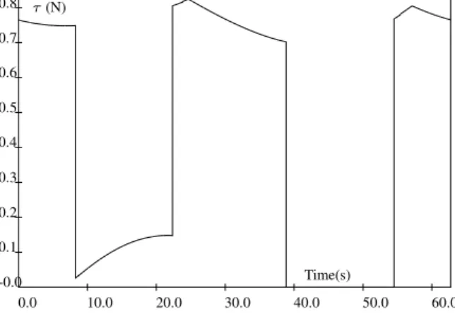
We have used the third algorithm to fully simulate the motion of the robot along a horizontal circle centered at (0,0,2) with radius 1 with an orientation such that the vectors of the reference and mobile frame were identi-cal. The velocity of the robot was set to 0.1m/s. It was supposed that the starting point of the trajectory was (1,0,2) with the configuration 345678. On this trajectory 11 changes of cable configurations were detected: 2 with only 5 cables under tension (34678, 13478 that occurred both twice on the trajectory) and 9 with 6 cables under ten-sion (345678, 234567, 134678, 134568, 125678, 124578, 123678, 123478, 123456). The CC with only 5 cables un-der tension occur only for a small amount of time, typically less than 1 ms. Figure 4 shows the tension of cable 3 during the trajectory while figure 5 shows the tension of cable 8. In both figures we can see the large influence of CC changes on the cable tensions.
0.0 10.0 20.0 30.0 40.0 50.0 60.0 -0.0 0.1 0.2 0.3 0.4 0.5 0.6 0.7 0.8 τ (N) Time(s)
Fig. 4. The tension in cable 3 along the circular trajectory
0 10 20 30 40 50 60 0.0 0.1 0.2 0.3 0.4 0.5 0.6 0.7 0.8 τ8(N) Time(s)
Fig. 5. The tension in cable 8 along the circular trajectory
We have timed the first and second algorithms for a max-imal changes of 2mm in the ρ, l0on this trajectory and the
computation time is usually less than 1ms which is satisfac-tory from a real-time point of view.
IV. Conclusions
This paper has addressed the real-time forward kinematic problem of CDPR i..e determining the pose of the robot af-ter a small change in its cable lengths, under the assumption that the cables have no mass but may or not have elasticity. This problem is more complex than the forward kinematics of parallel robots with rigid legs as the inverse kinematics equations that are used to solve the forward kinematics de-pends upon the cable configuration. Hence a forward kine-matic solver should take into account the point that the ca-ble configuration at the final pose may be different from the one at the initial pose, thereby leading to different equations and consequently to a different final pose. We have pro-posed 3 algorithms for that purpose. one compute all pos-sible pose and cable configurations after completion of the change in the cable lengths. The second one performs the same job but also compute changes in cable configurations during the coiling. The last algorithm assumes a model for
the coiling process and determine the unique pose and cable configuration at the end of the coiling. All three algorithms are basically real time in the sense that they complete within a sampling period of the controller. The results of the FK solver show that drastic changes in the cable tensions may occur due to CC changes. As classical simulation tools will ignore these changes they may underestimate positioning errors and cable tensions.
An interesting problem will be to determine if the third algorithm is able to deal with the sequence presented in fig-ure 3: during the large motion that leads from the CC with 4 cables under tension to a new stable CC with 6 cables under tension there is most probably no solution to the FK equations that respect the mechanical equilibrium. In that case it will be necessary to take into account the dynamics of the CDPR.
The presented algorithm do not deal with cables having significant mass and submitted to sagging. However in that case there is a single set of FK equations and the method described in [21] may be used after an adaptation to the sag-ging equations with either a simplified model [30], a mixed model [31] or a full model [22]. Surprisingly the real-time inverse kinematics may be more difficult for CDPR with sagging cables as our preliminary experiments have shown, but that has to be confirmed, that in some cases this prob-lem may not have an exact solution, in which case it will be necessary to determine a solution that is the ”closest” in some sense to the desired pose.
Another extension that has to be considered is toward non suspended CDPR. Here the downward pulling cables may be controlled in tension to ensure that all cables are under tension using strategies that have been exposed in numer-ous works [32], [33], [34], [35] but we believe that still there will be poses in the workspace for which cables may become slack. Finally it may also be necesseray to incor-porate interference detection in the real-time FK [36], [37], [38].
V. Annex: Kantorovitch theorem
Assume that we have a square system of n equationsF in the n unknowns x1, . . . , xn:
F = {Fi(x1, . . . , xn) = 0, i ∈ [1, n]}
LetX0 = {x01, . . . , x0n} be a vector of specific values for
the unknowns and define a ball U centered atX0with
ra-dius B0. We denote||G|| the norm of a vector or a matrix
G of dimension p or p × p. This norm may be arbitrary but we will use hereMax(|Gi|)∀i ∈ [1, p] for vectors and
Max(Pj=pj=1|Gij|)∀i ∈ [1, p]. Let’s assume that the
follow-ing conditions hold:
1. the Jacobian matrix of the system has an inverseΓ0at
X0such that||Γ0|| ≤ A0 2. ||Γ0F(X0)|| ≤ 2B0 3. Pnk=1|∂ 2 Fi(X ∂xj∂xk| ≤ C for i, j = 1, . . . , n and ∀X ∈ U
then if2nA0B0C ≤ 1 there is an unique solution of F in
U and the Newton method used withX0as initial estimate
of the solution will converge toward this solution.
Note that the last condition may be verified with interval analysis as soon as the unknowns are all bounded.
References
[1] Albus J., Bostelman R., and Dagalakis N. The NIST SPIDER, a robot crane. Journal of research of the National Institute of Stan-dards and Technology, 97(3):373–385, May 1992.
[2] Landsberger S.E. and Sheridan T.B. A new design for parallel link manipulator. In Proc. Systems, Man and Cybernetics Conf., pages 812–814, Tucson, 1985.
[3] Bruckman T. and others . Parallel manipulators, New Developments, chapter Wire robot part I, kinematics, analysis and design, pages 109–132. ITECH, April 2008.
[4] Jiang Q. and Kumar V. The inverse kinematics of 3-d towing. In ARK, pages 321–328, Piran, June 28- July 1, 2010.
[5] Roberts R.G., Graham T., and Lippit T. On the inverse kinematics, statics and fault tolerance of cable-suspended robots. J. of Robotic Systems, 15(10):581–597, 1998.
[6] Verhoeven R. Analysis of the workspace of tendon-based Stewart platforms. PhD thesis, University of Duisburg-Essen, Duisburg, 2004.
[7] Abbasnejad G. and Carricato M. Real solutions of the direct geometrico-static problem of underconstrained cable-driven paral-lel robot with 3 cables: a numerical investigation. Meccanica, 473(7):1761–1773, 2012.
[8] Berti A., Merlet J-P., and Carricato M. Solving the direct geometrico-static problem of the 3-3 cable-driven parallel robots by interval analysis: preliminary results. In 1st Int. Conf. on cable-driven parallel robots (CableCon), pages 251–268, Stuttgart, September, 3-4, 2012.
[9] Carricato M. and Merlet J-P. Direct geometrico-static problem of under-constrained cable-driven parallel robots with three cables. In IEEE Int. Conf. on Robotics and Automation, pages 3011–3017, Shangai, May, 9-13, 2011.
[10] Carricato M. and Abbasnejad G. Direct geometrico-static analysis of under-constrained cable-driven parallel robots with 4 cables. In 1st Int. Conf. on cable-driven parallel robots (CableCon), pages 269– 286, Stuttgart, September, 3-4, 2012.
[11] Pott A. An algorithm for real-time forward kinematics of cable-driven parallel robots. In ARK, pages 529–538, Piran, June 28- July 1, 2010.
[12] Carricato M. and Merlet J-P. Stability analysis of underconstrained cable-driven parallel robots. IEEE Trans. on Robotics, 29(1):288– 296, 2013.
[13] Pott A.. and others . IPAnema: a family of cable-driven parallel robots for industrial applications. In 1st Int. Conf. on cable-driven parallel robots (CableCon), pages 119–134, Stuttgart, September, 3-4, 2012.
[14] Tadokoro S. and others . A portable parallel manipulator for search and rescue at large-scale urban earthquakes and an identification al-gorithm for the installation in unstructured environments. In IEEE Int. Conf. on Intelligent Robots and Systems (IROS), pages 1222– 1227, Kyongju, October, 17-21, 1999.
[15] Merlet J-P. and Daney D. A portable, modular parallel wire crane for rescue operations. In IEEE Int. Conf. on Robotics and Automation, pages 2834–2839, Anchorage, May, 3-8, 2010.
[16] Su Y.X. and others . Development of a large parallel-cable manipu-lator for the feed-supporting system of a next-generation large radio telescope. J. of Robotic Systems, 18(11):633–643, 2001.
[17] Harshe M., Merlet J-P., Daney D., and Bennour S. A multi-sensors system for human motion measurement: Preliminary setup. In 13th IFToMM World Congress on the Theory of Machines and Mecha-nisms, Guanajuato, June, 19-25, 2011.
[18] Rosati G., Gallina P., and Masiero S. Design, implementation and clinical test of a wire-based robot for neurorehabilitation. IEEE Trans. on Neural Systems and Rehabilitation Engineering, 15(4):560–569, December 2007.
[19] Merlet J-P. MARIONET, a family of modular wire-driven parallel robots. In ARK, pages 53–62, Piran, June 28- July 1, 2010. [20] Dallej T., Andreff N., and Martinet P. Towards a generic
image-based visual servoing of parallel robots using legs observation. In 12th IFToMM World Congress on the Theory of Machines and Mech-anisms, Besancon, June, 18-21, 2007.
[21] Merlet J-P. Solving the forward kinematics of a Gough-type paral-lel manipulator with interval analysis. Int. J. of Robotics Research, 23(3):221–236, 2004.
[22] Merlet J-P. The forward kinematics of cable-driven parallel robots with sagging cables. In 2nd Int. Conf. on cable-driven parallel robots (CableCon), pages 3–16, Duisburg, August, 24-27, 2014. [23] Hansen E. Global optimization using interval analysis. Marcel
Dekker, 2004.
[24] Jaulin L., Kieffer M., Didrit O., and Walter E. Applied Interval Anal-ysis. Springer-Verlag, 2001.
[25] Moore R.E. Methods and Applications of Interval Analysis. SIAM Studies in Applied Mathematics, 1979.
[26] Neumaier A. Interval methods for systems of equations. Cambridge University Press, 1990.
[27] Knppel O. Profil/biasa fast interval library. Computing, 53(3-4):277– 287, 1994.
[28] Merlet J-P. ALIAS: an interval analysis based library for solving and analyzing system of equations. In SEA, Toulouse, June, 14-16, 2000.
[29] Fousse Laurent, Hanrot Guillaume, Lef`evre Vincent, P´elissier Patrick, and Zimmermann Paul. Mpfr: A multiple-precision bi-nary floating-point library with correct rounding. ACM Trans. Math. Softw., 33(2), 2007.
[30] Gouttefarde M. and others . Simplified static analysis of large-dimension parallel cable-driven robots. In IEEE Int. Conf. on Robotics and Automation, pages 2299–2305, Saint Paul, May, 14-18, 2012.
[31] Miermeister P. and others . An elastic cable model for cable-driven parallel robots including hysteresis effect. In 2nd Int. Conf. on cable-driven parallel robots (CableCon), pages 17–28, Duisburg, August, 24-27, 2014.
[32] Bruckmann T., Pott A., and Hiller M. Calculating force distributions for redundantly actuated tendon-based Stewart platforms. In ARK, pages 403–412, Ljubljana, June, 26-29, 2006.
[33] Diao X. and Ma O. Force closure analysis of 6 dof cable manipu-lators with seven or more cables. Robotica, 27(2):209–215, March 2009.
[34] Hassan M. and Khajepour A. Minimum-norm solution for the ac-tuator forces in cable-based parallel manipulators based on convex optimization. In IEEE Int. Conf. on Robotics and Automation, pages 1498–1503, Roma, April, 10-14, 2007.
[35] Lamaury J. and others . Design and control of a redundant sus-pended cable-driven parallel robot. In ARK, pages 237–244, Inns-bruck, June, 25-28, 2012.
[36] Blanchet L. and Merlet J-P. Interference detection for cable-driven parallel robots (CDPRs). In IEEE/ASME Int. Conf. on Advanced Intelligent Mechatronics, pages 1413–1418, Besancon, July, 8-11, 2014.
[37] Merlet J-P. Analysis of the influence of wire interference on the workspace of wire robots. In ARK, pages 211–218, Sestri-Levante, June 28- July 1, 2004.
[38] Y. Wischnitzer, Shvalb N., and Shoham M. Wire-driven parallel robot: permitting collisions between wires. Int. J. of Robotics Re-search, 27(9):1007–1026, September 2008.