HAL Id: hal-02535529
https://hal.archives-ouvertes.fr/hal-02535529
Submitted on 10 Apr 2020
HAL is a multi-disciplinary open access
archive for the deposit and dissemination of
sci-entific research documents, whether they are
pub-lished or not. The documents may come from
teaching and research institutions in France or
abroad, or from public or private research centers.
L’archive ouverte pluridisciplinaire HAL, est
destinée au dépôt et à la diffusion de documents
scientifiques de niveau recherche, publiés ou non,
émanant des établissements d’enseignement et de
recherche français ou étrangers, des laboratoires
publics ou privés.
Distributed under a Creative Commons Attribution - NonCommercial - NoDerivatives| 4.0
International License
Bastien Boussau, Celine Scornavacca
To cite this version:
Bastien Boussau, Celine Scornavacca. Reconciling Gene trees with Species Trees. Scornavacca, Celine;
Delsuc, Frédéric; Galtier, Nicolas. Phylogenetics in the Genomic Era, No commercial publisher |
Authors open access book, pp.3.2:1–3.2:23, 2020. �hal-02535529�
Trees
Bastien Boussau
Laboratoire de Biométrie et Biologie Évolutive (LBBE)
Université de Lyon, Université Lyon 1, CNRS, Villeurbanne, France [email protected]
https://orcid.org/0000-0003-0776-4460
Celine Scornavacca
Institut des Sciences de l’Évolution Université de Montpellier, CNRS, IRD, EPHE Place Eugène Bataillon 34095
Montpellier Cedex 05, France [email protected]
Abstract
In the last decade, we witnessed the ascent of reconciliations as an important tool to model and study the evolution of gene families. Reconciliations model discordance between gene trees and species trees caused by gene-level processes: duplications, losses and transfers of genes, Incomplete Lineage Sorting among others can be combined to generate a panoply of different models. In this review article, we give an overview of this vast topic by skimming over the different models and methods that have been proposed, and presenting some of their applications in phylogenomics. We also present the pros and cons of these methods and give some directions for future research that we are convinced will enhance their efficiency and use.
How to cite: Bastien Boussau and Celine Scornavacca (2020). Reconciling Gene trees with Species Trees. In Scornavacca, C., Delsuc, F., and Galtier, N., editors, Phylogenetics in the
Genomic Era, chapter No. 3.2, pp. 3.2:1–3.2:23. No commercial publisher | Authors open access
book. The book is freely available at https://hal.inria.fr/PGE.
1
Gene trees differ from species trees
When studying genome evolution in a set of species, it is often necessary to study the evolution of individual genes that are found across all or most of the species of interest. Assuming genome sequences are available and have been annotated, the first step of such an analysis is to define gene families. Those gene families group together homologous sequences, which are likely to have evolved from a common ancestral sequence. In some cases, there will be exactly one gene per species, in others, some species will be missing the gene, or some species will have more than one copy of the gene. Families with one gene copy per species are typically combined to reconstruct species trees. They can also be subjected to individual phylogenetic analyses, whose steps typically involve aligning the sequences and reconstructing their phylogeny, called a gene tree.
When such an analysis is performed, one often observes that many of the reconstructed gene trees do not agree with the (supposedly known) species tree. Here it is important to agree on what is meant by “agreement” between a gene alignment and a reference tree. The measure of disagreement should not be simply topological: a gene tree can differ from the species tree, but not significantly so. To conclude that a gene alignment really rejects a particular tree, a statistical test needs to be performed. Significant gene tree/species tree
discordances can have two main causes: either they reflect inferential errors or model mis-specification, or are due to evolutionary events that have led to truly different topologies between individual gene trees and the species tree.
1.1
Conflicts caused by errors and model inadequacy
Problems can arise at each step of a typical phylogenetic pipeline (see Chapter 2.1 [Simion et al. 2020]). First of all, the sequences themselves can be erroneous: for instance contam-ination is an issue whose importance has often been underestimated (Simion et al., 2018), and assembly errors are common too. Second, errors can occur during the construction of gene families. It is indeed easy for clustering methods for homology detection to miss a gene if its sequence has diverged a lot compared to the threshold that the user has chosen. Similarly, a gene that contains several protein domains1 may be incorrectly assigned to a
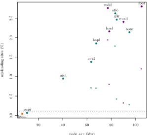
gene family with which it shares one of its domains, but not the others. In both cases, gene trees reconstructed from gene families where such clustering errors have occurred will likely be different from the species tree. One should work towards avoiding such mistakes, for in-stance by incorporating models of domain fusion/fission during the clustering and alignment steps. Once gene families have been defined, users typically want to extract families of ortho-logous genes (see Chapter 2.4 [Fernández et al. 2020]), i.e. remove paraortho-logous (=generated by duplication) and xenologous (=generated by transfer) gene copies. However, orthology relationships can be incorrectly inferred, in which case the analysis will be conducted on a group of sequences containing paralogs or xenologs; this may lead to cases as the ones depic-ted in Figures 2 and 3. Even when orthology is correctly inferred, errors can creep in at the next step, when the sequences are aligned, which may lead to phylogenetic reconstruction errors (see Chapter 2.2 [Ranwez and Chantret 2020]). Finally, our models of sequence evol-ution are simplistic and for instance very rarely account for dependencies between sites, and heterogeneities of the process across lineages or across sites. Such limitations can introduce errors during phylogenetic reconstruction. For all these reasons, we may observe a high level of discrepancy even in gene families where lateral gene transfers/duplications/losses and reticulate evolution (see Section 1.2) are rare or inexistant. For instance, in birds the amount of discord between gene trees was massive (Jarvis et al., 2015), and similarly in mammals (Scornavacca and Galtier, 2017). In such cases, it is often argued (e.g. in Song et al. 2012; Chapter 3.3 [Rannala et al. 2020]), that a large portion of this incongruence is due to incomplete lineage sorting (ILS, see Figure 4 and the associated section). However, in mammals, using simulations and back-of-the-envelope computations, Scornavacca and Galtier (2017) showed that ILS can only explain a small portion of the incongruence present in the data, see Figure 1. Additionally, in the bird phylogenomic data set, the amount of conflict between trees is larger when the trees are built from exon sequences than when the trees are built from intron sequences, even when the alignment size is taken into account. This result suggests that much incongruence is due to lack of information in the sequences, because exons are typically shorter and more constrained than introns.
1.2
Conflicts caused by biological processes
In this section, we briefly review the biological processes that can generate a gene tree different from the species tree (for more detailed reviews, see Maddison, 1997; Szöllősi et al.,
1 Protein domains are conserved parts of a given protein sequence that have the characteristics to be
● ● ● ● ● ● ● ● ● ● ● ● 20 40 60 80 100 0.0 0.5 1.0 1.5 2.0 2.5
node age (Myr)
mi sl ea di ng si te s (% ) homi root bore afro papi hapl rodd glireuad cetd arct laud
Figure 1 High levels of incongruence present in the OrthoMaM database. Dots correspond to
the proportion of parsimoniously-misleading sites for various ancestral nodes in the mammalian phylogeny, and the horizontal line shows the maximal expected percentage of ILS-induced incon-gruence. Reproduction of Figure 4 in Scornavacca and Galtier (2017), see corresponding paper for more details.
2015). To ease the reading, in our examples we will focus on evolutionary scenarios that generate gene families with exactly one gene per species. However, several of these processes can change copy numbers in a genome, and we will point this out in the description below when relevant.
1.2.1
Gene duplication and gene loss
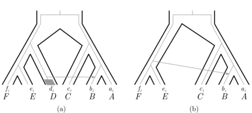
Gene duplication creates a new copy of a gene, at a different locus in the genome. When gene duplication is followed by gene losses, this may result in a gene tree differing from the species tree even when every extant species ends up with exactly one gene copy. For example, Figure 2(a) depicts a species tree (bold lines) inside of which the evolutionary history of a gene (grey lines) is drawn: first, a speciation happens in R, then the gene is duplicated in the branch leading to U followed by speciations in U and V . This scenario gives rise to seven different genes2a
1, a2, b1, b2, c1, c2, d. Now, if a2, b1, c2are lost, a1, b2, c1, d
may be wrongly identified as orthologs, leading to the tree in Figure 2(b), whose topology differs from that of the species tree (black lines in Figure 2(a)).
1.2.2
Gene transfer, gene conversion
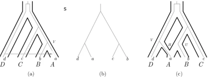
Differences in the topologies of a species tree and a gene tree can be caused by a combination of horizontal gene transfer and gene loss, as shown in Figure 3(a): the copy of the gene present in the ancestral species labelled by V is lost in the species labelled by a and it is replaced by a copy transferred from the species labelled by d. This gives rise to the topology in Figure 3(b), again conflicting with the topology of the species tree.
2 In the examples of this chapter, we will use the following notation: gene names are associated to
small-case letters, possibly subscripted by a number, and species names to capital letters, where genes belong to the species that is associated to the same letter.
Dd Cc1 c2 Bb1 b2 Aa1 a2 (a) a2 c1 b2 d (b) U R V
Figure 2 (a) A species tree (bold lines) along with a gene history (grey lines) involving
speci-ations, a gene duplication and gene losses (copies a2, b1 and c2 are lost). (b) The gene tree that
may be reconstructed from the data issued from the gene history in (a).
Dd C c Bb Aa (a) b c a d (b) V Dd A a Bb Cc (c) H V U s
Figure 3 (a) A species tree (bold lines) along with a gene history (grey lines) involving
spe-ciations, a gene transfer and a gene loss. (b) The tree that may be reconstructed from a gene alignement resulting from the gene history depicted in (a) or the one depicted in (c). (c) A species network (bold lines) along with a gene history (grey lines) involving a reticulation event.
Most methods assume that a gene transfer adds a new gene copy into the recipient genome. Some documented mechanisms of genetic exchange between genomes, however, involve replacement transfer, i.e., cases when the transferred gene is copied onto an existing homologous copy in the recipient genome by gene conversion. Such an event could result in the topology of Figure 3(b) without the need of any loss event: the recipient genome both gains the transferred copy and loses the resident copy at the same time. In such a case, classical models of gene transfer would typically reconstruct two events when a single one actually occurred (but see Suchard, 2005; Hasic and Tannier, 2017a, for exceptions). Of note, such replacement transfer events, which rely on sequence homology, are only expected to happen between closely related species.
1.2.3
Hybridization
The topology in Figure 3(b) can also be obtained by a scenario involving hybridization, whereby the genome of a descendant lineage is some type of fusion of the genomes of two parental lineages (see Figure 3(c)). Hybridization is increasingly recognized as having an key role in the evolution of some plants and animals, for example in wheat (Glémin et al., 2019) or yeasts (Morales and Dujon, 2012). In this case, the copy of the gene labelled by a is inherited from the ancestral species labelled by V ; no copy is inherited from U . Such processes result in dozens to thousands of replacement transfers, occurring through homologous recombination. Because they occur on such different scales and because in some cases hybridization can be associated with a duplication of the genetic material, replacement
transfers and hybridization have classically been modelled differently (Huson et al., 2010; Szöllősi et al., 2015).
1.2.4
Incomplete lineage sorting
Another possible source of conflict between species trees and gene trees is ILS (see Figure 4; Chapters 3.3 and 3.4 [Rannala et al. 2020; Bryant and Hahn 2020]).
c1c2c3c4
(a)
(b)
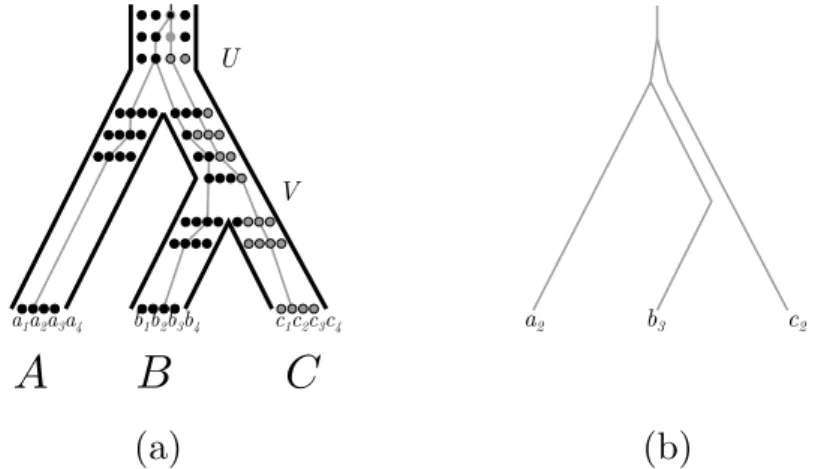
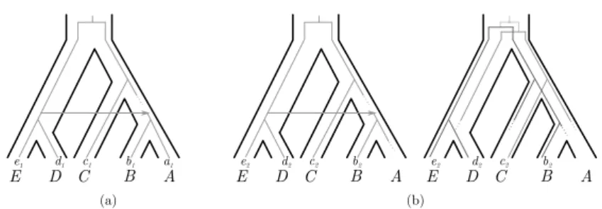
U V b1b2b3b4 a1a2a3a4 a2 b3 c2Figure 4 (a) A species tree (bold lines) along with the coalescent history of gene variants a2, b3
and c2(grey lines), descended from alleles present in the common ancestral population U . (b) The
gene tree that may be reconstructed from the data issued from the coalescent history depicted in (a).
In this figure, each population contains 4 individuals, each individual is represented with a dot whose color corresponds to a particular allelic form at a given locus, i.e. the black allele and the grey allele. The starting population contains a single allele. First, a mutation leads to a new grey allele at this locus, then a first speciation takes place in U , rapidly followed by a second one in V . As the black and grey alleles still co-exist in V , both alleles still have a chance to be fixed in B and C, so we can obtain the gene tree in Figure 4(b). It is important to realize that such a scenario is entirely neutral: there is no need to assume differences in fitness between the grey and black alleles for such an incongruence to occur. In fact, incomplete lineage sorting can occur whenever speciations occur closely enough that polymorphisms are not entirely “sorted out” between two speciations. Two parameters control the likelihood of such a scenario: first, how fast successive speciations occur. Second, how large the effective population sizes are: in populations with large effective sizes, there will be more polymorphism that stay longer in the population, and therefore more opportunities for ILS.
1.3
Better models to improve gene trees
Discordance between gene trees and species tree, therefore, can result from a variety of processes in combination, and it is often difficult to pinpoint one major cause. One can use better alignment tools and methods to detect contamination and reduce the amount of errors. Other factors can be addressed by improved models of sequence or gene family evolution. For instance, models of sequence evolution that incorporate heterogeneity between sites typically do better than models that treat all sites homogeneously (Lartillot and Philippe, 2004; Wang et al., 2018). Similarly, models that account for the across-lineage variation in
the substitution process should be able to perform better than the most usual models when data show substantial compositional heterogeneity (Boussau and Gouy, 2006; Heaps et al., 2014). Therefore, in practice, efforts should be made to use the most appropriate models of sequence evolution. In this review, we choose to focus on another approach to improve the accuracy of gene and species trees: gene tree-species tree (GTST) models. These models formally describe how a gene family evolves along a species tree and are the focus of the next section.
2
Gene tree-species tree (GTST) models
GTST models describe the evolution of gene trees along species trees, by placing gene duplication (D), transfer (T), loss (L) and conversion (C) events along the gene tree and ILS events along the species tree.
These models can be used in a variety of settings. Historically, people have been using these models in the reconciliation setting: the input typically consists of a gene tree and a species tree, and we look for the best scenario that embeds the gene tree inside the species tree, as shown in the figures of the previous section. The aim here may be to estimate the parameters of a given probabilistic GTST model (for instance, the rates of duplication and loss, or population genetic parameters of a model of ILS) or to map events onto the phylogeny (e.g., where the duplications and transfers are placed in the gene history). But these models can also be used to estimate gene trees. In this case, the input is the species tree and data from the genes of interest (e.g. a distribution of gene trees previously reconstructed from the genes, or the gene sequences themselves) and we use an algorithm to look for the gene trees giving the best reconciliation according to some scoring function. The hope is that using a species tree in addition to sequence information will result in an improved estimate of gene trees.
We shall start, after a short digression on parsimony and probabilistic approaches for GTST models (Section 2.1), by reviewing GTST models in the reconciliation setting (Sec-tion 2.2) and their extension to account for unsampled species (Sec(Sec-tion 2.3) and scenario uncertainty (Section 2.4). Finally, we will show how these models can be used to improve the accuracy of gene trees (Section 2.5).
2.1
Parsimony vs probabilistic models
Parsimony approaches have first been used for phylogenetic inference based on morphological or sequence data. Given a set of possible events and a cost for each of them, these methods aim at returning a solution that minimizes a cost function. For phylogenetic inference based only on sequence alignments, the cost function to minimize is usually the sum of the individual costs of events of substitution required to explain the evolution of the sequences along a particular tree topology. For GTST models in the reconciliation setting, the cost function would be the sum of individual costs of events of gene family evolution (typically duplications, losses, transfers or ILS) required to explain the evolution of a gene tree along a particular species tree. In both cases, the costs associated to the events have to be fixed by the user and cannot be estimated.
Probabilistic methods rely on a different type of cost function. Events are associated no longer to costs but to rates, which can be used to compute the probability of various evolutionary scenarios. For example, given rates for all the events considered, probabilistic GTST models in the gene tree-estimation setting (see Section 2.5) enable computing the likelihood of a gene tree, which is proportional to the probability of the gene tree given the
species tree; the posterior probability of a gene tree can be computed by combining the likelihood with prior probability distributions on parameter values. With such probabil-istic models, it is possible to estimate the parameters by identifying those maximizing the likelihood of a gene tree. Alternatively, one can integrate over the parameter distribution through Bayesian approaches, and generate the posterior probability of the gene trees and associated parameter values.
2.2
The reconciliation setting
The first and possibly best-known GTST model is the DL model:
IDefinition 1. Given a rooted gene tree G and a rooted species tree S whose species contain the genes in G, the evolution of G along S is subject to the following constraints:
1. Speciations are the only possible events shaping species histories;
2. Speciation, duplication (D) and loss (L) are the possible events shaping gene histories; 3. Each speciation in G happens at a speciation in S;
4. L events in G are supposed to happen just after a speciation in S;
5. Each speciation and D event in G gives birth to exactly two genes; 6. The evolution of G along S goes forward in time;
7. Each contemporary gene is a leaf of G and is associated to the corresponding species of
S in which this gene is collected.
See the Supplementary Material of Jacox et al. (2016) for a formal and mathematical definition of the model. A DL reconciliation is a plunging of G in S respecting Def. 1. This plunging can be formalised as a function that maps each node of G onto an ordered sequence of nodes of S.
If we are in the MP framework, we will seek the scenario minimizing the cost δ × |D| + λ × |L|, where δ and |D|, and λ and |L|, are respectively the cost and number of events in the scenario for duplications and losses. For this simple model, the best scenario is the Last Common Ancestor (LCA) mapping which can be found in linear time in |G| (Chauve and El-Mabrouk, 2009). In the ML or Bayesian framework, we will compute probabilities of scenarios described via birth-death processes (birth at speciation and duplication events and death at gene losses); in some cases, we may be interested in searching for the scenario with the highest probabilities, in others we can integrate over all scenarios to compute the probability that a given gene tree has evolved along a particular species tree, without explicitly specifying a particular scenario.
This simple model can be made more complex by considering other events shaping the gene history, for example gene transfer. When incorporating gene transfer, Point 2 of Def. 1 becomes:
2. Speciation, duplication (D), loss (L) and transfers (T ) between sampled/unsampled species are the possible events shaping gene histories;
We call this model, the DTL model. Because transfers necessarily occur between contempor-aneous species, transfers to older species are forbidden. However, when some species have not been sampled, it is possible to infer transfers from an ancient donor to a more recent recipient, even if the two species did not live at the same time. This is because a gene may have been transferred to species that are unrepresented in the sample under consideration. If a gene gets transferred to an unrepresented species, stays there for some time, then gets transferred into a lineage ancestral to a sampled species, it will look like a single transfer oc-curred between two represented lineages that did not live at the same time. This translates as follows:
8. Each T event happens between two coexisting species if transfers are allowed only between sampled species and their ancestors; otherwise, the donor simply has to be older than the recipient.
X T
Y Z
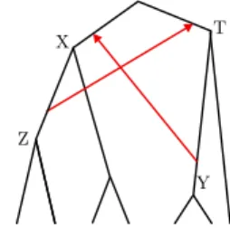
Figure 5 An example of a time-inconsistent scenario: we cannot have node X older than node
T and at the same time T older than X.
Now, because of Point 8 of Def. 1, each transfer implies a time constraint between a pair of nodes that may contradict the time constraints implied by other transfers. Computationally, the time constraints implied by gene transfers introduce additional complexity in ensuring Point 6 of Def. 1. Scenarios violating this point are called time-inconsistent and can be obtained within a single gene family, especially if it contains several gene copies. An example of a time inconsistent scenario that can be obtained by this latter approach is given in Figure 5. Avoiding time-inconsistent scenarios while preserving optimality is an NP-hard problem (Tofigh et al., 2011), even in the case where we have to reconcile a single binary gene tree with a binary species tree. (Interestingly, one can even make use of time-inconsistent scenarios across gene families to date a species tree, see Section 3.7).
To address this difficulty, two approaches have been used. Either reconciliation is per-formed against an undated species tree, and one can just hope that time inconsistencies will be rare. Or reconciliation is performed against a dated species tree: all scenarios are therefore consistent with the ages of the nodes of the species tree.
The model can be made even more complex by adding gene conversion (Hasic and Tannier, 2017a), allowing ILS (Vernot et al., 2008; Chan et al., 2017), and accepting un-rooted/non binary species and gene trees as input (Górecki and Tiuryn, 2007; Lafond et al., 2016, for instance).
2.3
Transfers to and from the dead
Many models only consider events between branches that have led to extant genes or species. However, much of the past diversity has left no descendant nowadays, and our sampling is necessarily incomplete. For those two reasons, it is likely that a large proportion of the transfers we detect have occurred with a species that has left no descendant among the leaves of our data set. When interpreting reconciled gene histories, it is important to keep this in mind, as this can lead to mistakes. In particular, although transfers necessarily occur between contemporaneous species, the fact that many species have not been sampled means that many donor species will be found on older branches than the sampled recipient species. An example is shown in Figure 6.
Accounting for unsampled species during inference with gene transfer can be done both in a parsimony and a probabilistic framework. In both frameworks, one has to make sure that transfers from a donor on an old branch of the tree can be received by recipients on any branch that is of the same age or more recent than the donor. In the probabilistic framework, one can then model unrepresented species. To this end, an additional modelling
C c1 B A (a) E D b1 a1 f1 e1 d1 F C c1 B A (b) E b1 a1 f1 e1 F
Figure 6 (a) An evolutionary scenario for a gene involving a transfer from the unsampled (or
extinct) taxon D. Since D is not present, the transfer is inferred to come from the ancestor of f1
and e1, see (b).
layer describing the total number of species living through time must be developed. Szöllősi et al. (2013b) assumed that species evolved according to a Moran model: the number of spe-cies vastly outnumbered the extant sampled spespe-cies but was constant through time. Other models that would allow variations in the number of species through time could be designed. Overall, with this additional layer, GTST models acquire an additional hierarchical level: sequences evolve along gene trees, which evolve with species trees, which are a subsample of an evolving population of species.
In a parsimony model, things are easier. For example, transfers to and from the dead are modelled in ecceTERA as follows: a “dummy” species is added to the species tree, and duplications, losses and transfers to it are free of cost, while transfers from it cost as ordinary transfers. The rational behind this choice is the following: the “dummy” species models all unsampled species thus it can duplicate and loose genes to mimic the number of unsampled species we need; transfers to the “dummy” species are free because they cannot be distinguished from undetected speciation events (undetected because the species became extinct/has not been sampled), while transfers from it are actual transfers.
2.4
Accounting for scenario uncertainty
Whether inference is performed in a parsimony or probabilistic framework, there are cases where several scenarios are nearly equally good descriptors of the evolution of a particular gene tree given a species tree. This would typically occur in a parsimony framework when several scenarios have the same total cost, but this can also occur in a probabilistic framework when several scenarios have very similar likelihoods or probabilities. In such cases, it is important that the reconciliation method returns more than a single scenario, so that the user is fully aware of the uncertainty associated to the inferred events. To put it differently: if a method always returns a single scenario, a user cannot tell if a particular event is necessary to explain a gene tree given a species tree, or if it is just one possible event out of many similarly likely events. If a single scenario is output, a user may well over-interpret an event that is highly uncertain. Another reason for returning several scenarios is depicted in Figure 7: one may be able to choose the preferred scenario among the returned ones using external information, in our example the reconciliation of a neighboring gene family suggesting a single transfer that involved both genes.
This is why almost all reconciliation tools nowadays have opted to show the uncertainty in the scenarios, either providing a measure of support for each event or a posterior distri-bution of scenarios.
C c1 B A (a) E D d1 e1 b1 a1 C c2 B A (b) E D d2 e2 b2 C c2 B A E D d2 e2 b2
Figure 7 Two sets of reconciliations for two different gene families containing respectively the
genes a1, b1, c1, d1, e1and b2, c2, d2, e2. (a) A scenario for the first family involving a transfer and a
loss. (b) Two different scenarios for the second family; the first invokes a transfer and a loss, the second a duplication and four losses. These two scenarios can have the same cost for some vectors of parameters, e.g. if transfers cost four and duplications and losses one, but the first scenario implies a single transfer event that would have moved both genes at the same time.
2.5
Taking into account gene tree uncertainty and improving gene tree
accuracy
Beyond uncertainty in the scenario explaining a gene tree given a species tree, there can be huge uncertainty in the gene tree itself. For this reason, it is common practice when inferring gene trees to compute branch support values, for instance through bootstrap (MP, ML), approximations of the bootstrap (ML), or by displaying posterior probabilities on branches (PP). For single gene trees, these support values can be quite low, which shows that there is a lot of uncertainty about the gene tree topology, and which forces interpretations to take branch support into account. Similarly, when inferring gene trees using GTST models, it is very important to take this uncertainty into account.
The two approaches that have been used to take this uncertainty into account in GTST programs are detailed below. In both cases, the program needs a species tree. Then, either the program uses gene sequences to output a distribution of gene trees, or the program takes as input a pre-existing distribution of gene trees, that it will alter and then output. Gene tree estimation based on GTST models can be seen as an effort to come up with an estimation of gene trees that balances between the information provided by the species tree and the information provided by sequence alignments. Hence, there is a choice to be made as to the weights associated to each of these two sources of information: a large weight on the species tree will cause all gene trees to resemble the species tree, while a large weight on sequence information will result in the same trees as obtained using PhyML, RAxML, IQtree, etc, all approaches that only rely on sequence information.
2.5.1
Approaches that take gene sequences as input
Those approaches require using a model of sequence evolution jointly with a GTST model. In a parsimony framework, this requires coming up with a meaningful choice of weights that balances the cost of a substitution with the cost of a duplication, loss, transfer or ILS. In a probabilistic framework, this means that both the parameters of the model of sequence evol-ution and the parameters of the model of gene family evolevol-ution have to be estimated. This creates a challenging problem, because the gene tree also has to be estimated. In addition, computing the likelihood of a gene tree according to an alignment is computationally costly,
which makes these methods time-consuming. An example of this approach is the software jPrIME-DLRS (Sjöstrand et al., 2012). Very recently, two new tools have been proposed for this task: Treerecs (Comte et al., 2019) and GeneRax (Morel et al., 2020), under the DL and DTL model respectively.
2.5.2
Approaches that take gene tree distributions as input
To simplify the inferential problem, several programs rely on input sets of gene trees which have been pre-computed from an alignment of gene sequences. Such sets can be obtained with bootstrap replicates, or thanks to Bayesian inference, in which case the set of trees approximates a probabilistic distribution on gene trees. Typically, such a distribution would be obtained with software for Bayesian gene tree reconstruction, such as MrBayes (Ronquist and Huelsenbeck, 2003), PhyloBayes (Lartillot et al., 2013) and Beast (Suchard et al., 2018). Based on such a set of trees, programs can search for the tree minimizing the cost or maximizing its probability according to a GTST model, or can sample trees according to their probabilities. Relying on a set of trees necessarily comes with a trade-off between accuracy and computational efficiency. If the tree distribution were infinite in size, all the information present in the alignment and exploitable by the model of sequence evolution would be enclosed in the tree distribution, and this approach would be entirely equivalent to the approach described in Section 2.5.1. Of course, the tree distribution has to have a finite size, and therefore cannot describe all the information present in the alignment. The larger the size of the tree distribution, the more accurate the inference will be, but it will also be more costly. In practice, authors have found good trade-offs between accuracy and speed (Edwards et al., 2007; Szöllősi et al., 2013a; Scornavacca et al., 2014), relying notably on the amalgamation idea.
Amalgamation, initially proposed in the parsimony framework by David and Alm (2011) and later formalised and extended to the probabilistic framework (Scornavacca et al., 2014; Szöllősi et al., 2013a), exploits the following ideas. First, a distribution G of trees induces a distribution of subtrees, which are obtained by cutting the complete trees on each of their internal branches. Second, given a distribution of subtrees, one can mix and match (am-algamate) subtrees with non-overlapping sets of tips to re-create complete trees. Third, provided one computes a few count statistics on the subtrees, it is even possible during this amalgamation step to recapitulate with high accuracy the frequency with which a particular complete tree has been observed in the tree distribution G, i.e. its conditional clade
probabil-ity (CCP). See Figure 8 for an example of amalgamation. Further, this amalgamation trick
can also be used to compute the probability of a complete tree that is not present in the input distribution, but can be obtained by amalgamating subtrees found in distinct input trees (Höhna and Drummond, 2011; Larget, 2013). Amalgamation is used in some GTST implementations to integrate over the topological uncertainty associated with the limited information contained in an alignment. Through a single pass of a dynamic programming algorithm, one can integrate over all this uncertainty, either in a parsimony (Scornavacca et al., 2014) or in a probabilistic framework (Szöllősi et al., 2013a).
A note on “overfitting” or shrinkage risk
As pointed out earlier, when using reconciliation to estimate gene trees under a parsimony framework, a reconciled gene tree is a barycentric estimate between a gene tree based on the sequences alone, and a gene tree based on the minimization of the number of e.g. D, T, L events. It can be difficult to place the barycenter. When the reconstructed gene trees tend
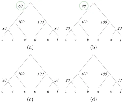
(a)
a b c d e f 80 a c b e d f 20(c)
a b c e d f 80 a c b d e f(b)
(d)
80 100 100 20 20 100 100 80 20 100 100 20 80 100 100Figure 8 An example of application of the amalgamation principle in the parsimony
frame-work and under the DL model. In (a,b) are presented the trees of our initial distribution, the first present 80 times and the second 20. In (c,d) are depicted the two trees that are not in the initial distribution but can be obtained via amalgamation of the trees in (a,b). The numbers next to the internal nodes show the occurrence of the corresponding clades in the initial distri-bution. Suppose that our species tree is the tree in (c) and δ, λ and w are respectively the cost of a duplication, the cost of a loss and the weight of the contribution of the sequence alignment to the cost. If the scoring function used is the one presented by Scornavacca et al. (2014), then the costs of the four trees are respectively (a) δ + 3λ +w × (2log(80/100) + 2log(100/100)), (b)
δ + 3λ +w × (2log(20/100) + 2log(100/100)), (c)w × (log(80/100) + log(20/100) + 2log(100/100))
and (d) 2δ + 6λ +w × (log(20/100) + log(80/100) + 2log(100/100)). (The terms in grey quantify the cost of deviating from the phylogeny preferred by the sequence alignment alone, while the ones in black are the reconciliation cost, which quantify the deviation of the gene tree from the species tree). Under some sets of weights, trees in (c) and (d) will have good scores even though they have never been observed in the input alignment.
to become too similar to the species tree, some authors have said that we are ”overfitting”
the species tree3. One could wonder whether the methods described in Section 2.5 suffer from overfitting since they deviate from the signal contained in the sequence alignment to embrace that of the species tree. In practice, Figure 2(a) of Scornavacca et al. (2014) shows that, for most of the existing methods, this is not the case. Also, if needed, users can choose a relative weight of the sequence component with respect to the reconciliation component of the joint score to avoid excessive shrinkage.
For the list of reconciliation tools in the parsimony framework, see Table 1 by Jacox
3 Actually, using the statistical jargon, it is probably more correct to say that the method “shrinks”
the estimate of the gene trees too much, because then each gene tree is “shrunk” to look like the species tree. After all, in regression, overfitting is used to describe a different phenomenon: when a line is drawn that passes through every single point instead of defining a central tendency, which is very similar to a situation where every single gene tree is allowed to have its own tree with its own idiosyncratic topology and parameters.
et al. (2016). This table is only slightly outdated. RANGER-DTL v.2.0 now permits taking as input unrooted and non-binary trees, Mowgli now accounts for ecological traits and ecceTERA for non-binary trees and for ILS, and EUCALYPT provides support values. For a list of published reconciliation tools in the probabilistic framework, see Figure 5 of Szöllősi et al. (2015).
3
Current/future directions
In this section, we will list several lines of research that may help spread the usage of reconciliation tools.
3.1
Mixing parsimony and probabilistic approaches
The major advantage of probabilistic models is that they allow estimating parameters in a proper statistical framework. Maximum likelihood is most appropriate when data is abund-ant, in which case the maximum of the function is well defined and the parameter values have small confidence intervals. When data is scarce, Bayesian methods –relying on integration– are more robust, because they attempt to integrate over all the uncertainty surrounding parameter values. The two approaches differ in their speed: Maximum Likelihood is usu-ally faster than Bayesian integration. But both are typicusu-ally much slower than parsimony approaches, which have no parameter to optimize (see Table 1).
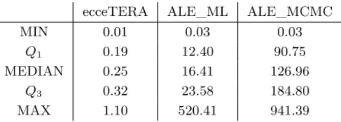
ecceTERA ALE_ML ALE_MCMC
MIN 0.01 0.03 0.03
Q1 0.19 12.40 90.75
MEDIAN 0.25 16.41 126.96
Q3 0.32 23.58 184.80
MAX 1.10 520.41 941.39
Table 1 Running times in seconds for three different methods –ecceTERA (Jacox et al., 2016),
ALE_ML (Szöllősi et al., 2013a) and ALE_MCMC (Szöllősi and Boussau, 2018), respectively a parsimony, ML and Bayesian method– on a dataset of 1099 homologous gene families present in 36 cyanobacterial genomes (the mean number of genes per family in the dataset is 36.66, the largest family has 114 genes and the smallest 21 genes, see Szöllősi et al., 2013a, for more details).
Although parsimony and probabilistic approaches differ in their treatment of the para-meters, they share important similarities in the algorithms used to compute the cost func-tions. In both cases, the algorithms often involve dynamic programming performed during tree traversals. In the field of gene tree reconstruction based on gene sequences only, many efficient algorithms combine probabilistic and parsimony approaches to benefit from their distinct qualities. Probabilistic models are used to operate in a sound statistical framework, which offers guarantees about the inference. Parsimony is used to speed up the algorithms and provide pretty good solutions fast. For instance, RAxML relies on parsimony to gen-erate starting trees (Stamatakis, 2006), and MrBayes 3.2 has a “parsimony-biased” SPR move (Ronquist et al., 2012). So far, reconciliation methods have not completely merged the parsimony and likelihood frameworks, but we believe there would be much opportunity for doing so. As described above for approaches that rely on sequence information only, new algorithms could be developed that would benefit from the speed of the parsimony cost function to more efficiently optimize or integrate a probabilistic cost function, i.e. the
likelihood or posterior probability of a gene tree. Alternatively, one could use algorithms such as importance sampling, where one samples parameter values from a quick-to-compute distribution, computes the probability of those parameter values using a more complex dis-tribution, and finally applies some simple reweighing of the initial distribution to obtain an unbiased sample from the more complex distribution. More specifically for GTST models, one could sample gene trees from a GTST parsimony model, compute their probability ac-cording to a sophisticated probabilistic model while sampling values of the parameters of the probabilistic model that were not present in the parsimony model, and finally reweigh the initial sample to obtain a sample of gene trees according to the sophisticated probab-ilistic model. For such a solution to be useful, sampling from the parsimony model should produce gene trees that have good probabilities, and the sampling of the parameters of the probabilistic model should not be computationally too costly.
3.2
Using reconciliation to estimate species trees
GTST models have also been used to score species trees. When combined with an algorithm that explores species tree topologies, this allows sampling species trees or finding the best species tree according to a particular GTST model based on a large number of gene families from the genomes of interest. Such an approach therefore potentially relies on a huge amount of data, and can bypass the need to identify families of orthologous genes, since D, T, L models can handle families with more than one gene copy per species (i.e. homologous genes). When the focus is on the species tree, it can be unnecessary to obtain individual gene family reconciliation scenarios. In fact, it becomes desirable to integrate over all possible reconciliation scenarios between the gene family and the species tree, and obtain a probability or a score that such a gene family would have evolved along a given species tree, irrespective of what particular events were involved, and on which branches they occurred. Such a probability or score is easy to compute using dynamic programming algorithms, which can integrate over or maximize a score or probability without any change to their structure. This approach has for instance been used in PHYLDOG (Boussau et al., 2013). Alternatively, in MCMC algorithms that sample parameters from probabilistic models, integration over all reconciliation scenarios can also be performed by sampling different scenarios at each step of the MCMC. The choice between these two methodologies would come down to which is most efficient to run, since they are equally difficult to implement. To speed up species tree inference in an ML framework, Ullah et al. (2015) have proposed a two-step algorithm whereby a set of candidate species trees built from families of orthologous genes is evaluated according to a DL probabilistic model. An approach combining fast parsimony methods with probabilistic inference as discussed in the previous section could also be a valuable option here.
3.3
Gene conversion vs gene transfer
As pointed out in the first section, gene conversion is not modelled well by most models of gene transfer, because it is a type of replacement transfer. To the exception of the model by Suchard (2005), all the models of transfer consider that a gene transfer adds a copy of a gene to a recipient genome. In those models, gene conversion has to be modelled by two events, a gene transfer and a gene loss. Gene families in which events of gene conversion have occurred will therefore have very unlikely scenarios according to most models of gene transfer, as they will require twice the number of events that actually occurred. In such cases, the barycentric estimation of the gene tree could be off: the GTST model will push
too much towards gene trees that resemble the species tree, because any difference costs twice as much as it should. For this reason, modelling accurately gene families with events of gene conversion would require developing a new model. Such a development is difficult: replacement transfers or gene conversions introduce dependencies between otherwise inde-pendent branches of the species tree, which breaks dynamic programming algorithms, the workhorses of all GTST methods. The model of replacement transfer (Suchard, 2005) uses a different type of algorithm, but is extremely limited in the size of the data sets it can handle. Short of developing a better model of gene conversion, users of GTST methods have two options. First, they could try to mitigate the impact of such a model misspecification by tweaking the parameters controlling the penalty or the probability of transfers and losses. By making transfers and losses cost less, or be more probable, scenarios involving gene con-versions will be less unlikely. Second, they could use network methods, which are typically designed to describe cases of hybridization or genome-wide reticulation (see section 3.6). This solution requires setting parameters of reticulation, which are usually estimated using genome-wide data and will not be well estimated using a single gene family.
Very recent advances on modelling gene conversion as a single event in the parsimony framework (Hasic and Tannier, 2017a,b) give us hope that gene conversion will be soon better modelled by reconciliation methods.
3.4
Reconciliation of all processes together
It would be very convenient to have a method that can handle all the processes that make gene trees differ from species trees. Such a method could identify which processes are at work in a particular gene family, on particular branches of the species tree. Duplications, transfers and losses have already been merged together, both in parsimony and in probabilistic models (Szöllősi et al., 2013a; Scornavacca et al., 2014; Sjöstrand et al., 2014, among others); the same holds for combining DL with incomplete lineage sorting (Rasmussen and Kellis, 2012; Wu et al., 2014, even though with some simplistic assumptions on how gene duplication and ILS interact). These latter models add an extra hierarchical layer on top of typical DL models: sequences evolve along a gene tree, which evolves according to a coalescent process along a locus tree, which evolves according to a birth-death process along the species tree. This model could be extended to account for gene transfers as well. In the parsimony framework, similar efforts have been attempted, the most complete model being the one of (Chan et al., 2017), combining DTL with incomplete lineage sorting (this method does also oversimplified assumptions on the interaction between duplication and ILS).
As evoked in Section 3.3, so far no model has combined replacement transfers with typical models of DTL, because the classical dynamic programming algorithms cannot be used when replacement transfers are included.
3.5
Reconciliation of several loci together
Gene trees can be reconstructed one by one using GTST models. When probabilistic models are used, this typically involves estimating parameters of the GTST models, such as the rates of various events. This can be difficult on single gene families, where the amount of inform-ation is necessarily limited. In such cases, rates can be mis-estimated, and reconciliinform-ation scenarios can be wrong. To improve rate estimation, information could be gathered across gene families, by performing joint estimation of the rates. This would reduce stochastic errors, but could result in over-shrinkage effects, where outlier loci with atypical parameter values would be constrained to share the parameter values estimated on other gene families.
A balance between gene-based and genome-based estimation of the rates could be obtained by borrowing ideas from models of rate heterogeneity across sites (Yang, 1994). Such models estimate an average rate of evolution across all sites, but allow variation around the average by estimating an additional variance parameter. There could be additional variance para-meters to account for variation in the rates of D, T, L or incomplete lineage sorting across gene families.
Moreover, some events of gene family evolution affect more than one gene family at a time. For instance, duplication, transfer and loss events can affect a segment of the genome that contains several genes. To identify such events it is desirable to analyse several gene families jointly and reconstruct joint scenarios. This, however, is difficult to do. First, events af-fecting segments of the genome may involve different numbers of genes in different lineages of the species tree. Therefore either an arbitrary choice is made on the number of jointly analyzed genes, or one has to come up with a method that will find the appropriate number for each branch, or assume that co-evolving genes co-evolve throughout their history. A method that identifies co-evolving genes per branch and that uses this information to recon-struct their history would be difficult to design as it would need to consider a vast number of possibilities. Chan et al. (2013) adopted a two-step approach: first, gene families were reconciled individually, and then probabilities that two gene families co-evolved over their entire history were computed based on the individual evolutionary scenarios. This approach was able to recover co-evolving genes in a simulation.
Second, genomes do not remain collinear throughout their evolution: two genes could be neighbors in one genome, but far from each other in another. Therefore either one focuses on the few genes whose relative positions have remained constant throughout their evolution, or one has to use a model of how genes move across the genome. The latter approach has been used in a series of papers that describe models using synteny information to reconstruct ancestral genome structures (Bérard et al., 2012; Patterson et al., 2013; Semeria et al., 2015) that are described in more depths in Chapter 2.5 (Tannier et al. 2020). These methods take as input a (dated) species tree4, a set of reconciled gene trees and the set of extant
adjacencies. The output is a set of ancestral adjacencies that, combined, give the ancestral genome structures. Their underlying model permits the creation and the loss of adjacencies and looks for an adjacency history that is compatible with the given reconciled gene trees and minimizes the number of adjacency creations and adjacency losses. Obviously, it would be interesting to reconcile the gene trees and, at the same time, minimize adjacency creations and losses, but the problem seems to be very complex and it has been conjectured to be NP-hard. To this day, the complexity of this problem is still open, even if the proof for a related problem presented in a very recent paper (Delabre et al., 2018) could shed some light.
Third, the space of all possible events then increases: for instance, in addition to D, T, L of single gene events, one needs to include events of D, T, L of at least pairs of genes. Very recently, methods to take into account duplications and losses of several genes at once (the so-called segmental duplications and losses) have been proposed in the parsimony framework (Delabre et al., 2018; Dondi et al., 2018). Overall, the development of models that consider the coevolution of several genes at a time is quite complicated and results in algorithms of high complexity.
3.6
Reconciliation with a species network
When the species phylogeny includes reticulation events such as hybridizations, we talk about species networks. Species network inference will not be reviewed in this book but we refer to the excellent recent reviews of Degnan (2018) and Elworth et al. (2019). Here we only aim at highlighting the similarities between some of the approaches to infer networks and the reconciliation methods presented in this chapter. For example, the MDC (Minimizing Deep Coalescence, e.g. Yu et al., 2011), is implicitly based on a reconciliation model in a parsimony framework permitting speciation and ILS at the gene level, and speciation and hybridization at the species level. In more details, gene trees evolve inside the network via speciations (hybrid or not)–giving a set of possible trees associated to the network– and a given gene tree can be reconciled with each of these trees via speciation and ILS. The best reconciliation w.r.t. the network is then the most parsimonious one over all possible scenarios and trees inside the network. The same rationale underlies similar methods in the probabilistic framework (e.g. Yu et al., 2014; Zhang et al., 2017). These latter models are very time consuming. Other models explicitly extended the reconciliation model to species networks, e.g. To and Scornavacca (2015) for the DL model and Scornavacca et al. (2017) for the DTL model. These methods do not take ILS into account yet. Roughly speaking, they consist in replacing Point 1 of the model described in Section 2.2 with:
1. Speciations and hybridizations are the only possible events shaping species histories; These explicit models are extremely scalable but also very recent and they have yet to prove their worth.
3.7
Improved dating with reconciliation
Dating a species phylogeny is a difficult endeavour that usually involves using fossil calibra-tions with relaxed clock models of the rate of sequence evolution. Although much work has been devoted to such inferences, dating a tree remains difficult because disentangling rate and time is fundamentally very hard. Basically, one needs to estimate a rate and a length of time per branch, all this based on an estimate of their product, the branch length. One pos-sibility to improve the inference of dated phylogenies would be to include other events than just events of substitution. In particular, reconciliations notably allow identifying events of D, T, L and placing them on branches of the species phylogeny. One could use these estimated numbers of events on each branch of the phylogeny to better disentangle branch length and rates of evolution, because time will affect in a similar way events of substitution and D, T, L events, while the rates of those events may be partially uncorrelated. By using more events, one could thus better estimate dated phylogenies.
Another approach to improve dating based on reconciliations is to use individual transfer events on their own. Transfer events necessarily occur between contemporaneous species. Given that species sampling is necessarily incomplete, transfers can only indicate that the ancestor of a donor species is necessarily older than the descendant of a recipient species (see Figure 5). Yet, such an information tells us something on the relative age of two nodes in the species tree, and the detection of a transfer event can be translated into a time constraint between nodes of a phylogeny if the donor and a recipient can be identified. When a set of transfers is detected by interpreting the phylogenetic discordance between a gene tree and a species tree, the set of all deduced time constraints can be used to rank the species tree, i.e. order totally its internal nodes. Several genes can give contradicting information that needs to be sorted out (Chauve et al., 2017); still, it seems that transfers can be successful in providing insights into the timing of diversification of clades across the
tree of life (Davín et al., 2018). Combining this transfer-based information with relaxed clock models of sequence evolution and with fossil calibration could result in much more accurate dates for the tree of life, even in taxa/epochs where the fossil record is scant.
3.8
RecPhyloXML and reconciliation visualisation
Recently, a common effort of a consortium of researchers involved in reconciliation-related software development resulted in the introduction of an integrative and flexible format to describe reconciliations (Duchemin et al., 2018). The format is based on grammars extending the PhyloXML format, which is aimed at representing annotated trees in XML. Roughly, in RecPhyloXML the species tree and the reconciled gene tree are described in PhyloXML. Then, each node of the reconciled gene tree is associated to a set of nodes of the species tree via tags that specify the type of event (duplication, transfer, etc), the support and geographical annotations, for instance.
We are confident that RecPhyloXML will ease the development of generic software per-mitting to visualise and compare reconciliations, such as Sylvix (Chevenet et al., 2015) and the web interface http://phylariane.univ-lyon1.fr/recphyloxml/recphylovisu. In turn, this will help the spread of the usage of the reconciliation tools tremendously. The practitioners will not need anymore to spend hours trying to understand the different out-puts of different reconciliation tools; they will be able to easily compare them and choose the best software for their data.
3.9
Impact of reconciliation on other steps of the phylogenomic
pipeline
We have seen that GTST models can improve gene tree inference. It is known that using better guide trees, e.g. phylogenetic trees guiding how pairwise alignments are combined to obtain a multiple alignment, improves alignment inference (Liu et al., 2009). Therefore it seems likely that using a species tree with a GTST model could improve alignment inference, though not for all instances (see Chapter 2.3 [Ranwez and Delsuc 2020]). Similarly, clustering gene sequences into homologous gene families could benefit from the information coming from the species tree. Clustering methods typically rely on fixed thresholds to include a sequence into a cluster: if a sequence is similar enough to one or several sequences of a cluster, it is included in the cluster, if not, it is excluded. The reliance on such a fixed threshold could be relaxed with some knowledge of the structure of the species tree and of its branch lengths. For instance, one could normalize scores or adapt the threshold to the phylogenetic distance between the considered species as has been done by Emms and Kelly (2015). One could go even further by using reconciliations with models of gene duplication, transfer and loss. Such models would penalize families that are represented in a patchy way in the species phylogeny, in particular in clades where transfer rates are low. Indeed, patchy families would require large numbers of duplications and losses, which would be associated to a low reconciliation score. If we use the species tree for the clustering step, one could develop an iterative approach where a first clustering is used to generate a species tree, which is then used to re-cluster the genes, taking into account the species tree.
4
Conclusion
Several reconciliation methods have been developed these past few years. These allow in-ferring better gene trees and quantifying the impact of gene-level processes on genome
evol-ution. Progress remains to be made to integrate more processes together (e.g. DTL with ILS, hybridization and gene conversion for multiple genes) in a single inferential method, to allow for correlations between gene histories, and to speed up methods for species tree inference. But reconciliation methods can already contribute to a better understanding of many processes of molecular evolution, and could improve the accuracy of several steps of our phylogenomic pipelines.
References
Bérard, S., Gallien, C., Boussau, B., Szöllősi, G. J., Daubin, V., and Tannier, E. (2012). Evol-ution of gene neighborhoods within reconciled phylogenies. Bioinformatics, 28(18):i382– i388.
Boussau, B. and Gouy, M. (2006). Efficient likelihood computations with nonreversible models of evolution. Systematic Biology, 55(5):756–768.
Boussau, B., Szöllősi, G. J., Duret, L., Gouy, M., Tannier, E., and Daubin, V. (2013). Genome-scale coestimation of species and gene trees. Genome Research, 23(2):323–330. Bryant, D. and Hahn, M. W. (2020). The concatenation question. In Scornavacca, C.,
Delsuc, F., and Galtier, N., editors, Phylogenetics in the Genomic Era, chapter 3.4, pages 3.4:1–3.4:23. No commercial publisher | Authors open access book.
Chan, Y.-b., Ranwez, V., and Scornavacca, C. (2013). Reconciliation-based detection of co-evolving gene families. BMC bioinformatics, 14(1):332.
Chan, Y.-b., Ranwez, V., and Scornavacca, C. (2017). Inferring incomplete lineage sorting, duplications, transfers and losses with reconciliations. Journal of theoretical biology, 432:1– 13.
Chauve, C. and El-Mabrouk, N. (2009). New perspectives on gene family evolution: losses in reconciliation and a link with supertrees. In Annual International Conference on Research
in Computational Molecular Biology, pages 46–58. Springer.
Chauve, C., Rafiey, A., Davin, A., Scornavacca, C., Veber, P., Boussau, B., Szollosi, G., Daubin, V., and Tannier, E. (2017). Maxtic: Fast ranking of a phylogenetic tree by maximum time consistency with lateral gene transfers. Peer Community in Evolutionary
Biology.
Chevenet, F., Doyon, J.-P., Scornavacca, C., Jacox, E., Jousselin, E., and Berry, V. (2015). Sylvx: a viewer for phylogenetic tree reconciliations. Bioinformatics, 32(4):608–610. Comte, N., Morel, B., Hasic, D., Guéguen, L., Boussau, B., Daubin, V., Penel, S.,
Scornavacca, C., Gouy, M., Stamatakis, A., Tannier, E., and Parsons, D. P. (2019). Treerecs: an integrated phylogenetic tool, from sequences to reconciliations. bioRxiv,
https: // www. biorxiv. org/ content/ early/ 2019/ 10/ 11/ 782946 .
David, L. A. and Alm, E. J. (2011). Rapid evolutionary innovation during an archaean genetic expansion. Nature, 469(7328):93.
Davín, A. A., Tannier, E., Williams, T. A., Boussau, B., Daubin, V., and Szöllősi, G. J. (2018). Gene transfers can date the tree of life. Nature ecology & evolution, 2(5):904. Degnan, J. H. (2018). Modeling Hybridization Under the Network Multispecies Coalescent.
Systematic Biology, 67(5):786–799.
Delabre, M., El-Mabrouk, N., Huber, K. T., Lafond, M., Moulton, V., Noutahi, E., and Castellanos, M. S. (2018). Reconstructing the history of syntenies through super-reconciliation. In RECOMB International conference on Comparative Genomics, pages 179–195. Springer.
Dondi, R., Lafond, M., and Scornavacca, C. (2018). Reconciling Multiple Genes Trees via Segmental Duplications and Losses. In Parida, L. and Ukkonen, E., editors, 18th
Inter-national Workshop on Algorithms in Bioinformatics (WABI 2018), volume 113 of Leibniz International Proceedings in Informatics (LIPIcs), pages 5:1–5:16, Dagstuhl, Germany.
Schloss Dagstuhl–Leibniz-Zentrum fuer Informatik.
Duchemin, W., Gence, G., Arigon Chifolleau, A.-M., Arvestad, L., Bansal, M. S., Berry, V., Boussau, B., Chevenet, F., Comte, N., Davín, A. A., et al. (2018). Recphyloxml-a format for reconciled gene trees. Bioinformatics, 1:7.
Edwards, S. V., Liu, L., and Pearl, D. K. (2007). High-resolution species trees without concatenation. Proceedings of the National Academy of Sciences, 104(14):5936–5941. Elworth, R. A. L., Ogilvie, H. A., Zhu, J., and Nakhleh, L. (2019). Advances in
computa-tional methods for phylogenetic networks in the presence of hybridization. In Warnow, T., editor, Bioinformatics and Phylogenetics: Seminal Contributions of Bernard Moret, pages 317–360. Springer International Publishing, Cham.
Emms, D. M. and Kelly, S. (2015). Orthofinder: solving fundamental biases in whole gen-ome comparisons dramatically improves orthogroup inference accuracy. Gengen-ome biology, 16(1):157.
Fernández, R., Gabaldón, T., and Dessimoz, C. (2020). Orthology: Definitions, prediction, and impact on species phylogeny inference. In Scornavacca, C., Delsuc, F., and Galtier, N., editors, Phylogenetics in the Genomic Era, chapter 2.4, pages 2.4:1–2.4:14. No commercial publisher | Authors open access book.
Glémin, S., Scornavacca, C., Dainat, J., Burgarella, C., Viader, V., Ardisson, M., Sarah, G., Santoni, S., David, J., and Ranwez, V. (2019). Pervasive hybridizations in the history of wheat relatives. Science Advances, 5(5):eaav9188.
Górecki, P. and Tiuryn, J. (2007). Inferring phylogeny from whole genomes. Bioinformatics, 23(2):e116–e122.
Hasic, D. and Tannier, E. (2017a). Gene tree reconciliation including transfers with replace-ment is hard and fpt. arXiv preprint arXiv:1709.04459.
Hasic, D. and Tannier, E. (2017b). Gene tree species tree reconciliation with gene conversion.
arXiv preprint arXiv:1703.08950.
Heaps, S. E., Nye, T. M., Boys, R. J., Williams, T. A., and Embley, T. M. (2014). Bayesian modelling of compositional heterogeneity in molecular phylogenetics. Statistical
Applica-tions in Genetics and Molecular Biology, 13(5):589–609.
Höhna, S. and Drummond, A. J. (2011). Guided tree topology proposals for bayesian phylogenetic inference. Systematic Biology, 61(1):1–11.
Huson, D. H., Rupp, R., and Scornavacca, C. (2010). Phylogenetic networks: concepts,
algorithms and applications. Cambridge University Press.
Jacox, E., Chauve, C., Szöllősi, G. J., Ponty, Y., and Scornavacca, C. (2016). eccet-era: comprehensive gene tree-species tree reconciliation using parsimony. Bioinformatics, 32(13):2056–2058.
Jarvis, E. D., Mirarab, S., Aberer, A. J., Li, B., Houde, P., Li, C., Ho, S. Y. W., Faircloth, B. C., Nabholz, B., Howard, J. T., Suh, A., Weber, C. C., da Fonseca, R. R., Alfaro-Núñez, A., Narula, N., Liu, L., Burt, D., Ellegren, H., Edwards, S. V., Stamatakis, A., Mindell, D. P., Cracraft, J., Braun, E. L., Warnow, T., Jun, W., Gilbert, M. T. P., Zhang, G., and Consortium, T. A. P. (2015). Phylogenomic analyses data of the avian phylogenomics project. GigaScience, 4(1):s13742–014–0038–1.
Lafond, M., Noutahi, E., and El-Mabrouk, N. (2016). Efficient non-binary gene tree res-olution with weighted reconciliation cost. In LIPIcs-Leibniz International Proceedings in
Informatics, volume 54. Schloss Dagstuhl-Leibniz-Zentrum fuer Informatik.
Larget, B. (2013). The estimation of tree posterior probabilities using conditional clade probability distributions. Systematic Biology, 62(4):501–511.
Lartillot, N. and Philippe, H. (2004). A bayesian mixture model for across-site heterogeneit-ies in the amino-acid replacement process. Molecular Biology and Evolution, 21(6):1095– 1109.
Lartillot, N., Rodrigue, N., Stubbs, D., and Richer, J. (2013). Phylobayes mpi: phylogenetic reconstruction with infinite mixtures of profiles in a parallel environment. Systematic
Biology, 62(4):611–615.
Liu, K., Raghavan, S., Nelesen, S., Linder, C. R., and Warnow, T. (2009). Rapid and accurate large-scale coestimation of sequence alignments and phylogenetic trees. Science, 324(5934):1561–1564.
Maddison, W. P. (1997). Gene trees in species trees. Systematic Biology, 46(3):523–536. Morales, L. and Dujon, B. (2012). Evolutionary role of interspecies hybridization and genetic
exchanges in yeasts. Microbiology and Molecular Biology Reviews, 76(4):721–739. Morel, B., Kozlov, A. M., Stamatakis, A., and Szöllősi, G. J. (2020). Generax: A tool
for species tree-aware maximum likelihood based gene family tree inference under gene duplication, transfer, and loss. bioRxiv, https: // www. biorxiv. org/ content/ early/
2020/ 02/ 20/ 779066 .
Patterson, M., Szöllősi, G., Daubin, V., and Tannier, E. (2013). Lateral gene transfer, rearrangement, reconciliation. BMC bioinformatics, 14(15):S4.
Rannala, B., Edwards, S. V., Leaché, A., and Yang, Z. (2020). The multi-species coalescent model and species tree inference. In Scornavacca, C., Delsuc, F., and Galtier, N., edit-ors, Phylogenetics in the Genomic Era, chapter 3.3, pages 3.3:1–3.3:21. No commercial publisher | Authors open access book.
Ranwez, V. and Chantret, N. (2020). Strengths and limits of multiple sequence alignment and filtering methods. In Scornavacca, C., Delsuc, F., and Galtier, N., editors,
Phylo-genetics in the Genomic Era, chapter 2.2, pages 2.2:1–2.2:36. No commercial publisher |
Authors open access book.
Ranwez, V. and Delsuc, F. (2020). Accurate alignment of (meta)barcoding datasets using macse. In Scornavacca, C., Delsuc, F., and Galtier, N., editors, Phylogenetics in the
Genomic Era, chapter 2.3, pages 2.3:1–2.3:31. No commercial publisher | Authors open
access book.
Rasmussen, M. D. and Kellis, M. (2012). Unified modeling of gene duplication, loss, and coalescence using a locus tree. Genome research, pages gr–123901.
Ronquist, F. and Huelsenbeck, J. P. (2003). Mrbayes 3: Bayesian phylogenetic inference under mixed models. Bioinformatics, 19(12):1572–1574.
Ronquist, F., Teslenko, M., van der Mark, P., Ayres, D. L., Darling, A., Höhna, S., Larget, B., Liu, L., Suchard, M. A., and Huelsenbeck, J. P. (2012). Mrbayes 3.2: Efficient bayesian phylogenetic inference and model choice across a large model space. Systematic Biology, 61(3):539–542.
Scornavacca, C. and Galtier, N. (2017). Incomplete lineage sorting in mammalian phyloge-nomics. Systematic Biology, 66(1):112–120.
Scornavacca, C., Jacox, E., and Szöllősi, G. J. (2014). Joint amalgamation of most parsi-monious reconciled gene trees. Bioinformatics, 31(6):841–848.