HAL Id: hal-01819422
https://hal.uca.fr/hal-01819422
Submitted on 8 Feb 2021
HAL is a multi-disciplinary open access
archive for the deposit and dissemination of
sci-entific research documents, whether they are
pub-lished or not. The documents may come from
teaching and research institutions in France or
abroad, or from public or private research centers.
L’archive ouverte pluridisciplinaire HAL, est
destinée au dépôt et à la diffusion de documents
scientifiques de niveau recherche, publiés ou non,
émanant des établissements d’enseignement et de
recherche français ou étrangers, des laboratoires
publics ou privés.
Ozone nighttime recovery in the marine boundary layer:
Measurement and simulation of the ozone diurnal cycle
at Reunion Island
P. Bremaud, F. Taupin, A. Thompson, N. Chaumerliac
To cite this version:
P. Bremaud, F. Taupin, A. Thompson, N. Chaumerliac. Ozone nighttime recovery in the marine
boundary layer: Measurement and simulation of the ozone diurnal cycle at Reunion Island. Journal
of Geophysical Research: Atmospheres, American Geophysical Union, 1998, 103 (D3), pp.3463 - 3473.
�10.1029/97JD01972�. �hal-01819422�
JOURNAL OF GEOPHYSICAL RESEARCH, VOL. 103, NO. D3, PAGES 3463-3473, FEBRUARY 20, 1998
Ozone nighttime recovery in the marine boundary layer:
Measurement
and simulation
of the ozone
diurnal cycle at Reunion Island
P. J. Bremaud and F. Taupin
Laboratoire de Physique de l'Atmosphbre, Universit6 de la R6union, Cedex, France
A.M. Thompson
NASA Goddard Space Flight Center, Greenbelt, Maryland N. Chaumerliac
Laboratoire de M6tfiorologie Physique, Universit6 Blaise Pascal-CNRS, Clermont-Ferrand, France
Abstract. We describe the diurnal cycle of ozone in the marine boundary layer measured
at Reunion Island (21øS,
55øE) in the western part of the Indian Ocean in
August-September 1995. Results from a box chemistry model are compared with ozone
measurements
at Reunion Island. We focus on the peak-to-peak amplitude of ozone
concentration, since our measurements show a variation of about 4 parts per billion byvolume, which is close to the value obtained by Johnson
et al. [1990] during the Soviet-
American Gases and Aerosols
(SAGA) 1987 Indian Ocean cruise. Different dynamical
mechanisms are examined in order to reproduce such a variation. We conclude that the most important one is the exchange between the ozone-rich free troposphere and the ozone-poor boundary layer. This exchange is supposed to be more important during thenight than during the day, allowing ozone nighttime recovery.
This is the key point of the
observed diurnal cycle, since daytime ozone photochemistry is well described by themodel.
Then we assume
an entrainment
velocity
equal
to 1 mm s -• during
the day and 14
mm s
-• during
the night
to closely
match
our measurements.
Topography
influences,
together with clouds,
are presumed
to be responsible
for this difference between nighttime
and daytime
entrainment
velocities
of free tropospheric
air into the boundary
layer at
Reunion Island. Over the open ocean the difference of the turbulent flux of sensible heatbetween the day and the night explains
the strong ozone nighttime recovery
observed
by
us and by Johnson et al. [1990].1. Introduction
Several ozone measurements over the tropical open ocean show a diurnal cycle of ozone concentration between a maxi- mum at sunrise, a minimum in late afternoon, and a peak-to- peak variation of 10-15% corresponding to an absolute vari- ation equal to 3-4 parts per billion by volume (ppbv) [Oltmans,
1981; Piotrowicz et al., 1989; Johnson et al., 1990; Rhoads et al.,
1997]. We have recently found the same characteristic in our
measurements at Reunion Island.
In this study we show that we can reproduce this peak-to- peak variation of ozone by considering the capacity of ozone to recover at night through the exchange between the lower free troposphere (FT) and the marine boundary layer (MBL). At Reunion Island, local circulations induced by the interaction between trade winds and the high mountains can account for a more important vertical flux of 03 during the night than during the day, but it cannot be invoked to explain the strong ozone nighttime recovery observed over the open ocean.
In the first part of this paper (section 2) we describe the
measurements made at Reunion Island. Second, we examine Copyright 1998 by the American Geophysical Union.
Paper number 97JD01972.
0148-0227/9g/97JD-01972509.00
the photochemistry using a model that simulates Indian Ocean conditions. Although mean concentrations of many species appear reasonable, photochemical reactions do not reproduce the observed ozone diurnal cycle. In section 4 we consider whether dynamics can enhance ozone diurnal variations. It is shown that the local topography can contribute to stronger nighttime FT-MBL exchange relative to daytime. This mech- anism appears to provide additional day-night contrast to ac- count for the Reunion Island ozone data. Over the open ocean we show that the relative value between the night and the day of the turbulent flux of sensible heat can explain the strong ozone nighttime recovery observed in the tropical marine boundary layer by Johnson et al. [1990].
2. Experimental Data
The ozone diurnal variation experiment occurred from Au- gust 22 to September 4, 1995, during the austral winter, in the marine boundary layer at Reunion Island. Ozone measure- ments were taken using an electrochemical concentration cell
(ECC) sensor. This ECC sensor is an iodine/iodide redox cell,
with iodide ions being oxidized by ozone. An electrical current proportional to the quantity of ozone molecules pumped into the cell is generated. The ozone mixing ratio (ppbv) is calcu- lated from this current and depends on the total flow rate of
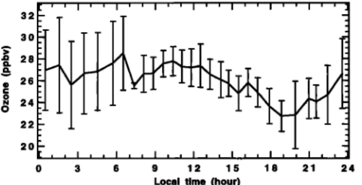
3464 BREMAUD ET AL.: OZONE NIGHTTIME RECOVERY IN THE BOUNDARY LAYER 32 3O •o 24 0 22 2O 0 3 6 9 12 15 18 21 24 Local time (hour)
Figure 1. Mean diurnal concentration of ozone measured at Reunion Island obtained by averaging the no-rain days.
the pump and the cell temperature. Simultaneous measure- ments of atmospheric temperature, pressure, and humidity were done. The relative precision of ECC sensor partial pres- sure measurements in the troposphere was found to be 6-10% by field test [Barnes et al., 1985; Hilsenrath et al., 1986].
The equipment was installed on the roof of one of the buildings on the University of Reunion Island in order to permit easier access to the electrochemical cells for their main- tenance. The University of Reunion Island is located at a height of about 200 m and is 2 km from the ocean. It is dominated essentially by easterly winds which come from the ocean.
Our measurements of ozone concentration at Reunion Is-
land were processed as follows: Measurements lasting 15 min were performed every 60 min. During each !5-min period, approximately 150 measurements were taken. The first 5 min are eliminated to allow for the adaptation time of the sensor. Then an average was done for each quarter hour, to obtain one measure per hour and to eliminate high frequencies. The ozone diurnal variation experiment extended for 14 days. Data from rainy days were eliminated because of the large ozone depletion which occurred. An average over the 10 remaining days provided a mean daytime series of ozone concentration (Figure 1), where a diurnal cycle is immediately observable, with a daily decrease during daylight hours and a strong night-
time recovery.
3. Photochemical Modeling of Reunion Data
In order to simulate the diurnal cycle of the trace gas con- centrations in the marine boundary layer, we use a time- dependent box model which describes the reaction scheme
NxOy - HxOy - CO - CH 4 (Table 1). In Table 1 the photo-
dissociation rates of each photoactive molecule (the J value) are calculated using a photochemistry model developed byMadronich [1987]. For our location of interest, photodissocia- tion rates are calculated using the date from the beginning of the simulation (October 10, 1992) and the latitude and longi- tude of Reunion Island (21øS, 55øE), i.e., over the tropical open Indian Ocean.
We assume clear-sky conditions, and the radiation calcula- tion includes an above-troposphere total ozone column of 270 Dobson units (DU), routinely obtained using a zenithal obser- vations analysis spectrometer (SAOZ) installed at Reunion Island [Denis et al., 1996], and a sea surface albedo of 0.07, a value characteristic of water surfaces [Jacob, 1986]. Since sev- eral reaction rate coefficients are temperature dependent, we
have simulated a diurnal cycle of temperature, with a minimum of 282 K just before sunset and a maximum of 291 K at the beginning of the afternoon.
We use an exponential method to solve the equation gov- erning the time evolution of gaseous concentrations of the different chemical species. This method, which has been re- cently used by Gr•goire et al. [1994], is 10 times faster than the Gear [1971] method and has been described by Chang et al. [1987].
Table 2 shows the conditions assumed for the model. Since
we did not measure the concentration of chemical species other than ozone at Reunion Island, we use, as guidance for the photochemistry modeling, chemical data from the Trans- port and Chemistry near the Equator in the Atlantic (TRACE-A) experiment, which took place as part of the Global Tropospheric Experiment (GTE).
This campaign included 19 flights over the Atlantic Ocean, on the coast of South America, and over Africa [Fishman et al., 1994]. The flight which interests us is the eleventh, which occurred between the African continent and Madagascar (22.3øS, 39.1øE/36.1øS, 30.7øE) on October 9, 1992 (Figure 2). This flight provided several measurements of temperature, hu-
midity, 03, NOx, NOy, HNO3, H202, CH4, CO, CO2,
CH302H, CH20, HCO2H, and NMHCs in the unpolluted marine boundary layer [He&es et al., 1996].
Since our study takes place at Reunion Island and the data were taken near South Africa, we justify the use of TRACE-A data by running backward trajectories from the location and the date of TRACE-A flight 11 (Figure 2). We use the three components of wind fields from the European Center for Me-
dium-Range Weather Forecasts (ECMWF), and possible di-
vergences in trajectories are reduced by running backward trajectories from points shifted from the arrival point by fixed amounts in latitude and longitude (_+0.5 ø latitude and +__0.5 ø longitude, respectively).
The marine origin of the air mass (Figure 2), together with the low concentration of 03, NOx, CH4, and CO, notably [Heikes et al., 1996] suggest that the TRACE-A chemical data, together with Reunion ozone data, form a coherent data set to simulate the photochemistry of ozone at Reunion Island.
4. Results and Discussion
4.1. Origin of Ozone Nighttime Recovery at Reunion Island Our measurements also show a maximum at sunrise, a min-
imum in late afternoon, and a rough peak-to-peak amplitude
of 4 ppbv (Figure 1). These results imply a daytime photo-
chemical destruction and a significant nighttime production of ozone. In view of the processes governing ozone concentration,
this production may be related to a nonphotochemical expla-
nation.
To some extent, the ozone diurnal cycle results from pho- tochemical processes. During the day, ozone concentration is closely tied to the NOx (NO + NO2) level, since the ozone formation is expected to be negative if NOx concentration is
low (less than 20 parts per trillion by volume (pptv); see Table
2), This condition is characteristic of a nonpolluted marine atmosphere such that we observe in the marine boundary layer of Reunion Island. Indeed, the reaction schemes (R1)-
(R104)-(R2), (R15)-(R13), and (R7) are more efficient than
the conversion of NO to NO2 (R18)-(R19), followed by
(R17)-(R101) when NOx concentration is low.
BREMAUD ET AL.: OZONE NIGHTTIME RECOVERY IN THE BOUNDARY LAYER 3465
Table 1. Reaction Scheme
Reaction
No. Reaction Notation
(R1) (R2) (R3) (R4) (R5) (R6) (R7) (R8) (R9) (R10) (Rll) (R12) (R13) (R14) (R16) (R17) (R18) (R19) (R20) (R21) (R22) (R23) (R24) (R25) (R26) (R27) (R28) (R29) (R30) (R31) (R32) (R33) (R34) (R35) (Rim) (R102) (R103) (R104) (R105)
0 3 q-
h v --> O
(1D)
q- 0 2
0 3 q- OH- --> HO 2 ß + 0 2 0 3 q- HO 2 ß --> OH' + 20 2 2HO 2 ß --> H20 2 + 0 2 H20 2 q- h v -• 2OH' H20 2 q- OH'--> HO 2 ß q- H20 CH4 + OH' + 02 + M --> CH30 2 ß + H20 + M CH30 2 ' + HO 2 ß --> CH302H + 0 2 CH302H + 0 2 + h v --> CH20 + HO 2 ß + OH' CH302H q- OH'--> CH30 2 ß + H20 CH302H + OH'--> CH20 + OH' + H20 CH20 + 20 2 + h v--> CO + 2HO 2 ß CH20 + h v--> CO + H 2 CH20 + OH' + 02 --> CO + HO 2 ß + H20 CO + OH' + 02 --> CO2 + HO2'NO + 0 3 •'> NO 2 + 0 2 NO 2 + h v--> NO + O NO + HO 2 ß -• NO2 + OH' NO + CH30 2 ß + 0 2 -'> NO 2 + CH20 + HO2' NO 2 + OH' + M -• HNO 3 + M HNO3 + hv--> NO 2 + OH' HNO 3 q- OH' --> NO 3 ß + H20 CH20 + HO 2 ß <--> O2CH2OH O2CH2OH + HO 2 ß --> HCO2H + H20 + 0 2 O2CH2OH + NO + 02 --> HCO2H + NO2 +
HO 2 ß
O2CH2OH + O2CH2OH --> 2HCO2H + 2HO 2 ß HCO2H + OH' + 02 --> CO2 + HO2' + H20 NO 3 ß q- hv--> NO + 02 NO 3 ß + h v --> NO 2 + O N205 + h v--> NO 2 + NO 3 ß NO 2 + 0 3 •'> NO 3 ß + 0 2 NO + NO 3 ß --• 2NO 2 NO 2 + NO 3 ß + M--> N20 5 + M N205 + M--> NO 2 + NO 3 ß + M N205 + h v-• NO + NO 3 ß + O O + 02 + M -• 0 3 + M O (1D) q- N 2 --> O + N 2 O (1D) q- 0 2 •'> O q- 0 2 O (lb) + H20 --> 2OH' 03+hv-->O + 02 diurnal variation 1.6 x 10⁻¹² exp (- 940/T) 1.1 x 10 -14 exp (-500/T) (2.3 x 10 -13 exp (600/T) + 1.7 x 10 -33 [M] exp (1000/T)) x (1 + 1.4 x 10 -21 [H20 ] exp (2200/ T)) diurnal variation 3.3 x 10⁻¹² exp (- 200/T) 2.3 x 10⁻¹² exp (- 1700/T) 4.0 x 10 -12 diurnal variation 5.6 x 10 -12 4.4 x 10 -12 diurnal variation diurnal variation 1.1 x 10 -11 2.3 x 10 -13 2.0 X 10⁻¹² exp (- 1400/T) diurnal variation 3.7 x 10 -12 exp (240/T) 4.2 x 10⁻¹² exp (180/T) 1.2 x 10 -11 diurnal variation 7.2 x 10 -ls exp (785/T) + 1.9 x 10 -33 [M] exp (725/T)/(1 + 1.9 x 10 -33 [m] exp (725/T)/(4.1 x 10 -16 exp (1440/T))) 6.7 x 10 -ls exp (450/T) 2.0 x 10 -12 7.0 x 10 -12 1.2 x 10 -13 3.2 x 10 -13 diurnal variation diurnal variation diurnal variation 1.4 X 10-- 13 exp (- 2500/T) 1.7 x 10 -11 exp (150/T) 8.1 x 10 -11 (T/300) -4'1 4.6 X 10¹⁶ (T/300) -4'4 exp (-11080/T) diurnal variation 6.0 X 10 -34 (T/300) -2'3 1.8 x 10 -11 exp (107/T) 3.2 x 10 -11 exp (67/T) 2.2 x 10 -1ø diurnal variation
Table 2. Model Conditions
One likely explanation is dynamics. Ozone nighttime recovery can take place by two different possible means [Paluch et al., 1992]: vertical transport through the inversion or horizontal transport from the descending branch of the Hadley cell near
30 ø south latitude by southeasterly wind. By these two ways,
free tropospheric ozone is introduced into the marine bound-
ary layer.
Lenschow et al. [1988] show results obtained during the Dy- namics and Chemistry of Marine Stratocumulus (DYCOMS) experiment by Kawa and Pearson [1989], who estimate an en- trainment velocity of dry O3-rich air of the free troposphere
Model Mean Daytime TRACE-A Observed
Species Mixing Ratio Mixing Ratio
0 3 29.1 ppbv OH 0.25 pptv HO 2 14.4 pptv H20 2 1.0 ppbv CH302 42 pptv NO 3.0 pptv NO 2 8.9 pptv HNO3 74 pptv NO 3 0.06 pptv N20 5 0.005 pptv 0.41 ppbv 69 ppbv 276 pptv 0.73 ppbv
into humid O3-1ow air of the marine boundary layer equal to 2 HCOOH
mm
s
-1 with
a range
of 1-5 mm
s
-1 in cloudy
conditions.
This
CO
entrainment
velocity
reflected
turbulence
processes
at the
top CH20
of the
boundary
layer
in the
presence
of stratocumulus.
At CH3OOH
28-31 ppbv not measured not measured 0.9-1.4 ppbv not measured 3.0-4.5 pptv 21-27 pptv 160-200 pptv not measured not measured 0.34-0.68 ppbv 67-74 ppbv 130-160 pptv 0.71-0.73 ppbv
3466 BREMAUD ET AL.: OZONE NIGHTTIME RECOVERY IN THE BOUNDARY LAYER
KIMEMRTIC TRRJECTORIES FRaM B2100906 TO B2100506
20 S
30 S
Figure
2. Backward
trajectories
starting
from 23
ø south
latitude
on October
9, 1992, using
the three
components
of wind
fields
from the European
Center
for Medium-Range
Weather
Forecasts
(ECMWF).
Reunion Island the presence of clouds is more important dur-ing the day than during the night, which is often cloud-free
during austral winter. This is due to the interaction between trade winds and Reunion Island mountains, which leads to the
formation of orographic clouds during the day on the slopes of the island and to their evaporation at night by downslope winds (Figure 3). However, Betts and Boers [1990] suggest that ver-
tical mixing across the inversion should be more efficient in
clear conditions than in cloudy conditions. This is due to a gradual temperature inversion in clear-sky conditions versus a
sharp inversion in the presence of clouds due to the enhance-
ment of turbulence in the upper part of the boundary layer. A decrease of the potential temperature gradient below the in- version results from this mixing, leading to sharp temperature jumps at the inversion [Paluch and Lenschow, 1991]. These thermodynamic profiles are commonly observed at Reunion Island, as shown in Figure 4, which depicts the vertical profiles
of potential temperature and dew point observed at Reunion
Island
in clear
conditions
on September
20, 1995
(Figure
4a),
and in cloudy
conditions
on October
5, 1995 (Figure
4b). In
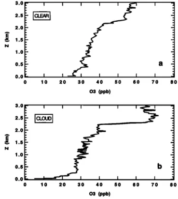
Figure 5, which shows the corresponding ozone profiles, it appears clearly that the ozone exchange between the lower free troposphere and the marine boundary layer at tempera- ture inversion level is very weak in cloudy conditions relative to clear conditions. Indeed, the strength of this exchange can becharacterized by the gradient of ozone concentration between
2.2 and 2.4 km (i.e., near the top of the marine boundary
layer),
which
is very strong
in cloudy
conditions
(Figure
5b),
reflecting
weak exchanges
relative
to clear conditions
(Figure
5a), where exchanges are more important.Donahue and Prinn [1990] suggest a sudden marine bound- ary layer deepening at dawn which would bring free tropo-
spheric air with high ozone concentration into the marine
boundary layer. In the case of a high island like Reunion
5000
2500
1 SO0
WESIE•MES
trade wind inversion
Reunion Island Mountains
•"""•
"
- Tr•ADE
WINDS
temperature inversion
Figure 3. Conceptual scheme of the interaction between Reunion Island mountains and southeasterlies
during
the night:
Land
breeze
downslope
winds
are enhanced
by bolster
eddies.
This figure
[from
Garret,
BREMAUD ET AL.: OZONE NIGHTTIME RECOVERY IN THE BOUNDARY LAYER 3467 3.0 2.5 2.0 N 1.0 0.5 0.0 I 8 12 16 I ' I ' I ' I * I ' I 20 24 28 32 36 40 O, 0 d(øC) 3.0 2.5 2.0 N 1.0 0.5 0.0 0 4 8 12 16 20 24 28 32 36 40 O, 0 d(øC)
Figure 4. Thermodynamic profiles on (a) September 20, 1995 (clear conditions); and (b) October 5, 1995 (cloudy con- ditions).
Island, another explanation can be proposed. Indeed, during the night, above and below the temperature inversion, bolster eddies resulting from the interaction between mountains and easterlies enhance the land breeze (Figure 3). During the night the combined action of easterly bolster eddies and land breeze downslope winds induces a mixing between ozone-rich air orig- inating from above the inversion and low ozone concentration air from the boundary layer, the region concerned being char-
acterized by weak unsteady and turbulent winds [Oke, 1978].
Moreover, the high mountains of Reunion Island force the lower tropospheric flow (southeasterlies) around them, since the much greater volume of easterlies relative to land breeze
demands that most of the mass flux be deflected around the
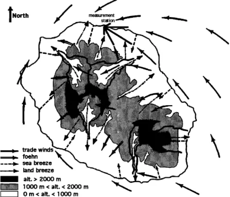
island (Figure 6) [Garrett, 1980; Ramage, 1978]. The air from the mixing region can be transported around the island, nota- bly over the north part of the island where we have done the 03
measurements, since the mean observed wind direction at the
station during the measurement period was east-southeast (Figure 7). This way of ozone nighttime recovery at the mea- surement station is not the only one, since the measurement station air can come directly from the just above lower free troposphere through the land breeze along the northern slopes of the island (Figure 6). This last case is generally observed
3.0 2.5 2.0 •.5 1.0 0.5 0.0 I o lO I I I 20 30 40
'/
I I I 50 60 70 03 (ppb) 3.0 2.5 2.0 •.5 1.0. I I I I I I •
.o.o, •
I
I
I
I
I
-
0 10 20 30 40 50 60 70 80 03 (ppb)Figure 5. Vertical ozone profiles on (a) September 20, 1995 (clear conditions), and October 5, 1995 (cloudy conditions).
during periods when trade winds are weaker than during the measurement period, which corresponds to the annual maxi- mum of trade wind strength.
The greatly enhanced nighttime variability which appears in Figure i is then tied to the dynamic origin of ozone nighttime recovery. Indeed, the strength and the time of establishment of these local circulations are highly variable following the large- scale conditions, especially the direction and strength of trade winds. Since the data have been simply averaged, the variability is enhanced during the night relative to the day, where the main driving parameter is the photochemistry, which does not vary from day to day in clear-sky conditions.
Ozone in the marine troposphere has an estimated photo- chemical lifetime of about 17 days [Liu et al., 1992], suggesting possible contamination at one particular location by long- range transport. However, Liu et al. [1992], observing the near balance between ozone production and loss at Mauna Loa Observatory, suggest that this balance controls the ozone con- centration such that transport processes would be negligible. Furthermore, as highlighted by Johnson et al. [1990], in the remote marine tropical atmosphere, both a high water vapor concentration and a large UV flux favor a shorter lifetime of ozone. Thus, under these climatological conditions, $mit et al. [1988] found approximately 4 days for 03 photochemical life- time. The timescale for ozone contamination through Hadley circulation is too long for the daily phenomenon we are look- ing at.
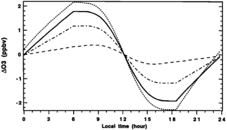
We assume that a more important vertical flux of 03 during the night than during the day is relevant for describing the 03 diurnal cycle. Indeed, using a constant entrainment velocity, the model does not simulate the measured 3-4 ppbv variation of ozone concentration (Figure 8, dashed line). The values 1
mm s -• (daytime)
and 14 mm s -• (nighttime)
associated
with
3468 BREMAUD ET AL.: OZONE NIGHTTIME RECOVERY IN THE BOUNDARY LAYER - trade • foehn ---•. sea breeze ... 4- land breeze --- alt, > 2000 m ß • ... 1000 rn < all < 2000 m I I Orn<alt.<lOOOm
Figure 6. Map of Reunion Island showing the location of the measurement station and the different observed winds. Solid arrows represent southeasterlies; open arrows show the location of foehn; dashed arrows show the location of sea breeze during the day: and the dash-dotted arrows show the location of land breeze during the night.
(Figure 5) [Baldy et al., 1996] closely match our measurements, whereas weaker nighttime entrainment velocities underesti- mate the ozone nighttime recovery and stronger nighttime
entrainment velocities lead to an overestimate of MBL ozone
concentration (Figure 8). Note that these diurnal cycles of
ozone variation are obtained after the simulation of several
diurnal cycles until convergence was obtained. We use the convergence criterion defined by Chameides [1984], i.e., a vari- ation by less than 1% of the noon concentration of all the species between two successive diurnal cycles.
Our daytime
entrainment
velocity
(1 mm s -1) can be com-
pared with the value of 1-5 mm s -1 deduced
by Kawa and
Pearson [1989] during the day. Our diurnally averaged entrain-
ment velocity
(7 mm s -x) lies between
the constant
value (5
mm s -1) assumed
by Heikes
et al. [1996] and the value esti-
mated byAnderson et al. [1993] between 1100 LT and 0010 LT
the next morning
(11 mm s- l).
4.2. Origin of Ozone Nighttime Recovery Over the Open
Ocean
First we have to examine the possibility of occurrence of the 3-4 ppbv of ozone nighttime recovery in the tropical marine boundary layer over the open ocean. Let us consider the ide- alized case depicted in Figure 9, where zi represents the top of the marine boundary layer, A0 is the strength of the tempera- ture inversion, q m and q t are the ozone concentration in the marine boundary layer and in the free troposphere, respec- tively, and Aq is the difference between qm and qt.
The turbulent fluxes of sensible heat at ground (mark 0) and at the mixed-layer top (mark e) are
Ho = pC.(w' 0')o (1) He = pCp(w' Ot)e (2)
respectively. Considering that the nocturnal tropical marine boundary layer is convective, the heat flux at the top of the mixed layer can be matched with the entrainment flux, and we have [Carson, 1973]
He • -aHo (3) where a is typically about 0.2.
We parameterize the cinematic fluxes of entrainment of heat and ozone using the following two equations:
( wt Ot)e • WeA 0 (4) (w' q')e • WeAq (5)
where w e is the mean entrainment velocity. Then we suppose that we have a net entrainment of free tropospheric air within the boundary layer.
Using (4) and (2) in (5), the cinematic flux of ozone entrain- ment can be approximated by
He Aq
(w'q')e
pep
A
0
(6)
If &q is the enhancement of ozone within the entire boundary layer,
BREMAUD ET AL.: OZONE NIGHTTIME RECOVERY IN THE BOUNDARY LAYER 3469 2500- 2000- 1500 - 1000- 500- a o -I , ,, -180 Wind Speed (m/s) 10 15 ' ' I ' ' ' ' I ' ' ' '
/
I , , I , , I , , I , , I , , -120 -60 0 60 120--I-- Wind Direction (Degrees from North)
2O 180 5OOO 4000 E 3000 N 2000 1000 0 -180
--A-- Wind Speed (m/s)
0 5 10 15 20
I [ i ! i i [ i i i i i '1 i i i
I , , I , , I , , I , , I , , I , , -120 -60 0 60 120 180
-•- Wind Direction (Degrees from North)
--A--Wind Speed (m/s) 0 -I 5000- . 4000- 3000- 2000- 1000- 5 10 15 20
,
, I
I
[ C•
, I • i I [ i I , &',
I , ,I I , , I
180 -120 -60 0 60 120 180 -I-- Wind Direction (Degrees from North)Figure 7. Mean wind speed and mean wind direction ob- served during the ozone measurement period at (a) 0400 LT, (b) 1000 LT, and (c) 1600 LT.
zi
A0 Aq
temperature qm qt
03 concentration
Figure 9. Idealized case of vertical profile of temperature
and ozone concentration.
(w'q')e
/Sq
=
Z,
(7)
we deduce from (7), (6), and (3) the following expression: H0 1 Aq
l•q
• a pCp
Zi A
0
(8)
Using the following values to describe the nocturnal tropical
marine
boundary
layer:
Ho •- 100 W m-2; a •- 0.2; pCp
1.3 x 10³ J m -3 K-•; Z i •- 1000 m;/Xq •. 15 ppbv;
and
• 3 K; we obtain •Sq •- 0.3 ppbv h -•. Then this value issufficient to recover 3-4 ppbv of ozone during the night. Nat- urally, this scheme is not strictly representative of the real vertical profiles of temperature and ozone concentration, but it allows us to examine the possibility of ozone nighttime recov- ery to match 3-4 ppbv. In particular, in order to simplify, we do not take humidity into account in this calculation. Neverthe- less, as highlighted by Wyngaard [1988], the entrainment- induced turbulence can extend through the mixed layer to the surface, particularly in the presence of high humidity.
If this strong ozone nighttime recovery is physically coher- ent, however, we have to examine why the FT-MBL exchange is stronger during the night than during the day. Looking at equation (8), we see that the parameters which are changing with time of day are A0 and H o. Indeed, the height of the marine boundary layer does not change between the day and
\ •... _ -- .-- -..
-1 ,, -..
-2
0 3 6 9 12 15 18 21 24
Local time (hour)
Figure 8. Simulated diurnal variation of ozone concentration using a daytime entrainment velocity equal to
! mm s -• and a nighttime
entrainment
velocity
equal
to I mm s -• (dashed
line), 5 mm s -• (dash-dotted
line),
14 mms
-• (solid
line), and 30 mm s -• (dotted
line).
3470 BREMAUD ET AL.: OZONE NIGHTTIME RECOVERY IN THE BOUNDARY LAYER
-2
0 3 6 9 12 15 18 21 24
Local time (hour)
Figure 10. Diurnal variation of ozone concentration measured during the SAGA 87 Indian Ocean cruise
[Johnson et al., 1990] (dashed line) and mean diurnal variation of simulated ozone concentration (solid line).
the night [LeMone, 1978], and we assume the same character- istic for Aq. The stronger daytime relative to nighttime tem- perature inversion (A0) due to nighttime cooling of the air above the inversion is a commonly accepted characteristic of the boundary layer evolution with time of day. The turbulent flux of sensible heat (Ho) is clearly stronger during the night than during the day over a warm ocean. Thus Moeng et al.
[1992]
defined
a flux equal
to 240 W m -2 for their simulation
of the clear nocturnal marine boundary layer, while most of the daytime measurements of this flux give a value between 10 and
30 W m -2 over the tropical
ocean
[LeMone,
1978].
Note that
for the above calculation, a more than twice reduced heat flux
(100 W m -2 against
240 W m -2) is sufficient
to match
the 3-4
ppbv of ozone nighttime recovery. The difference in heat flux between the day and the night can be explained by the fact that the ocean temperature remains constant (less than 0.5 degrees of variation) when the air temperature varies with time of day. The difference in temperature between the ocean and the air is stronger during the night, enhancing the turbulent flux of sensible heat. Moreover, the daytime radiative heat flux tends to decrease the net heating rate of the air in the boundary layer, leading to the reduction of daytime surface heat flux [Termekes, 1973].
Using a constant 1-km-depth boundary layer and assuming a
nighttime
entrainment
velocity
of 5 mm s-1 for the first hours
of the night, 14 mm s -• for the following night hours, and a daytime entrainment velocity of 1 mm s -•, our model simu-lates well both the ozone nighttime recovery and the daytime photochemical destruction relative to the Johnson et al. [1990] measurements (Figure 10). We have defined two nighttime
entrainment
velocities
(5 and 14 mms
-1) in order
to dosely
match the measurements. Indeed, they dearly show that the ozone nighttime recovery is stronger during the second part of the night relative to the first. This can be easily explained by the fact that the turbulent heat flux is weaker following dusk than before dawn in relation to the air-sea temperature differ- ence. In Figure 10 we can see that the model destroys ozone more rapidly than what is observed. We think that the averag- ing over 20 ø of latitude (10ø-30 ø south latitude) is the cause of this slower daytime photochemical destruction.
4.3. Related Photochemistry
In this section we will highlight the influence of the stronger nighttime FT-MBL exchange and the associated 3-4 ppbv of diurnal variation of ozone concentration on the diurnal cycle of related species. The results of our simulations will be com-
pared to TRACE-A data (Table 2). We will focus on charac-
teristics at remote maritime locations, especially in the tropics of the southern hemisphere.
Ozone 03. Integrating the diurnal cycle of ozone concentra-
tion (Figure 8, solid line), we calculate the "ozone production
potential" (OPP) using the following formula:
OPP = kls[NO][HO2] + k19[NO][CH302]- [03] ø {k2[OH] + k3[HO2]} - k10410(1D)][H2 ¸]
We find -3.7 ppbv 03 per day, for an average concentration equal to 29 ppbv 03. This value is coherent with the values calculated on Soviet-American Gases and Aerosols (SAGA) 3 by Thompson et al. [1993], since they find that the OPP in a low-NOx environment should be negative and that it is mainly dependent on the concentration of ozone. Note that the ratio OPP/mean[O3], i.e., the inverse of the photochemical lifetime of 03, is equal to 0.12 for our simulations and near the value 0.11 obtained by Thompson et al. [1993] at 10øN.
Nitric oxide NO, nitrogen dioxide NO2, and nitric acid
HNO 3. Whether ozone is formed or destroyed depends on the NOx (i.e., NO + NO2) concentration. Indeed, NO levels lower than ---10 pptv normally lead to the net destruction of ozone [Lelieveld and Crutzen, 1991; Thompson, 1994]. This corresponds to approximately 10-30 pptv of NOx, these con- ditions being generally characteristic of the nonpolluted ma- rine boundary layer. Our model simulations of the NO diurnal behavior give a mean daytime value of 3 pptv, which agrees with TRACE-A measurements (Table 2).
Note that the NO2 concentration measured on the TRACE-A flight is higher than that simulated by our model. We think that this strong concentration of NO2 relative to the NO low level is not characteristic of a pure marine boundary layer, since the NO2/NO ratio varies from 4.9 to 7.8 and the related HNO 3 concentration is too high. Indeed, the conver- sion of NO and NO2 to HNO 3 has a time constant of about 1 day, while the conversion of HNO 3 back to NO + NO2 re- quires 3-4 weeks [Logan et al., 1981]. So Torres and Thompson [1993] show that HNO3 buildup leads to a net loss of NOx, because HNO 3 acts as a reservoir compound having a 1- to 2-week lifetime, depending on aerosol or precipitation scav- enging rate. Therefore the high concentration of nitric acid on this part of TRACE-A flight 11 is not characteristic of a pure marine boundary layer but may result from a mixing between polluted free troposphere and boundary layer air.
BREMAUD ET AL.: OZONE NIGHTTIME RECOVERY IN THE BOUNDARY LAYER 3471 1.1 1.0 0.9 0.8 0.7 I ' ' / ' ' I ' ' I ' ' I ' ' I' ' ' I ' ' I ' ' • 0 3 6 9 12 15 18 21 24
Local time (hour)
Figure 11. Simulated diurnal cycle of H202 concentration.
1.0- .
0.9
0.80.7'.
- 0.6 0.5 0 3 6 9 12 15 18 21 24 Local time (hour)Figure 12. Simulated diurnal cycle of CH302H concentra-
tion.
which is less than TRACE-A data (160-200 pptv) but com- pares favorably with LeBel et al. [1990] measurements in the remote marine boundary layer during NASA/GTE/CITE 2 (Chemical Instrumentation Test and Evaluation) (62 pptv) and with GAMETAG (Global Atmospheric Measurements Exper- iment on Tropospheric Aerosols and Gases) measurements (70 pptv) [Huebert and Lazrus, 1980].
NO and NO 2 show strong diurnal variations, the first one being formed during the day, while the second is destroyed. These behaviors are in good agreement with Donahue and Prinn's [1990] simulations. However, during the night our sim- ulations show a replenishment of NO2, while Donahue and Prinn [1990] found a slight decrease. This is due to our as- sumption of stronger nighttime FT-MBL exchange, this source exceeding the sea surface deposition sink for NO2 during the night.
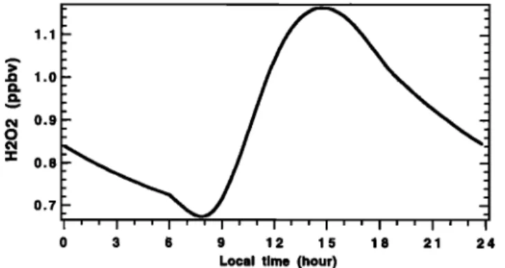
Hydrogen peroxide H20 2 and methylhydrogen peroxide
CH302 H. The diurnal variation of H202 is due to daytime formation of CH302 and HO2, balanced by the oxidation and photolysis of OH. We simulate a mean daytime mixing ratio of about 1.0 ppbv, which corresponds well to TRACE-A data (0.9-1.4 ppbv). Our simulated diurnal variation is comparable to that obtained by Thompson et al. [1993], showing a maxi-
mum in midafternoon and a minimum 2 hours after sunrise
(Figure 11), this minimum coinciding well with their measure- ments. However, we obtain a peak-to-peak amplitude multi- plied by 2.5 relative to the measurements showed by Thompson et al. [1993]. This is normal if we take into account that we simulate 1 ppbv of H202 and 4 ppbv of diurnal variation of 03 relative to 0.6 ppbv of H202 and 1 ppbv of diurnal variation of 03 on SAGA3, respectively. Indeed, the larger peak-to-peak amplitude can be correlated to that of 03 since H202 is formed from the reaction between two HO 2 molecules (reaction (R4), of which the large part is due to reactions involving OH (re- actions (R14)-(R15)), which is mainly produced by the pho- tolyric destruction of 03 (reactions (R1) and (R104)). Here then appears another important influence of the strong ozone nighttime recovery at Reunion Island.
The methylhydrogen peroxide (CH302H) mean daytime
concentration simulated by our model is 0.73 ppbv, which is in good agreement with TRACE-A data (Table 2). The simulated diurnal variations of CH302H (Figure 12) are similar to those simulated by Thompson et al. [1993] and to those observed on SAGA3, i.e., a minimum 2 hours after sunrise followed by a sharp buildup, leading to a maximum at about 1500 LT. How- ever, we find a peak-to-peak amplitude of 600 pptv against 200 pptv for Thompson et al. [1993] on SAGA 3. This higher peak-
to-peak amplitude can be correlated to that of 03 in the same way as for H202, considering CH302 in addition to HO2, pointing out another major influence of stronger nighttime FT-MBL exchange on marine boundary layer photochemistry.
Carbon monoxide CO. In the gas phase the reaction of CO with OH (reaction (R15)) is very important, since this reaction is the main sink for OH and for CO (80-90% for Novelli et al. [1992] and the unique CO sink in our model). The formation
of CO from CH20 (reactions (R12)-(R13)-(R14)) is the larg-
est known source of CO.
CO mixing ratios have often been measured in many regions
of the Earth. These measurements show that CO concentra-
tions vary both latitudinally and seasonally and that a realistic concentration for pristine oceanic air at 20 ø south is 55-70 ppbv [Novelli et al., 1992]. Our simulations show a mean day- time mixing ratio of 69 ppbv, which reproduces well the marine boundary layer TRACE-A data (67-74 ppbv).
We simulate a diurnal variation of about 2 ppbv CO, which agrees well with measured CO diurnal variations of tropical Pacific cruises [Johnson et al., 1991]. Only the assumption of stronger nighttime FT-MBL exchange relative to daytime ex- change, such as considered in our model, allows us to simulate this 2 ppbv of CO diurnal variation.
5. Summary and Conclusions
In this paper we focus on the marine boundary layer diurnal cycle of trace gas concentrations in relation to a strong night- time recovery of ozone. Indeed, both our measurements at Reunion Island and those of Johnson et al. [1990] show a sharp
decrease of ozone concentration between sunrise and the late
afternoon, with a variation of 3-4 ppbv. This variation is as- sociated with a significant ozone nighttime recovery, which can be explained by greater exchange during the night than during the day between the lower free troposphere and the marine boundary layer. Topographical influence can explain this strong nighttime FT-MBL exchange at Reunion Island, while stronger nighttime turbulent heat flux of sensible heat can be invoked over the open tropical ocean. Using a time-dependent box chemistry model, we have simulated well these observed diurnal variations of ozone considering an entrainment veloc-
ity of 1 mm s- • during the day and 14 mm s- • during the night.
We use data from flight 11 of TRACE-A between south of
Africa and Madagascar as guidance for our simulation of the
photochemistry of the marine boundary layer. Thus we have simulated the influence of this vertical exchange, which is more
3472 BREMAUD ET AL.: OZONE NIGHTTIME RECOVERY IN THE BOUNDARY LAYER
intense during the night than during the day, on the diurnal cycle of the other trace gases in the marine boundary layer. The main influence is observed on the diurnal cycles of H202, CH302H, and CO, since their peak-to-peak variations of con- centration are enhanced by a factor of 2-3 relative to previous measurements [Thompson et al., 1993]. This study, which tries to explain strong diurnal variations of several trace gas species in the marine boundary layer, leads us to plan more complete experiments at Reunion Island, including simultaneous mea- surements of at least 03, CO, H20 2, and CH302H, in order to further our understanding of the marine boundary layer pho- tochemistry.
Acknowledgments. We are indebted to B. Guillemet from Labo- ratoire de M•t•orologie Physique (France) for his help about marine boundary layer dynamics and to C. Bhugwant and J. Forsman for the editing of this manuscript.
References
Anderson, B. E., G. L. Gregory, J. D. W. Barrick, J. E. Collins, G. W. Sachse, C. H. Hudgins, J. D. Bradshaw, and S. T. Sandholm, Factors influencing dry season ozone distributions over the tropical South Atlantic, J. Geophys. Res., 98, 23,491-23,500, 1993.
Baldy, S., G. Ancellet, M. Bessaft, A. Badr, and D. Lan Sun Luk, Field observations of the vertical distribution of tropospheric ozone at the island of Reunion (southern tropics), J. Geophys. Res., 101, 23,835-
23,849, 1996.
Barnes, R. A., A. R. Bandy, and A. L. Torres, ECC ozonesonde accuracy and precision, J. Geophys. Res., 90, 7881-7888, 1985. Betts, A. K., and R. Boers, A cloudiness transition in a marine bound-
ary layer, J. Atmos. Sci., 47, 1480-1497, 1990.
Carson, D. J., The development of a dry inversion-capped convectively unstable boundary layer, Q. J. R. Meteorol. Soc., 99, 450-467, 1973. Chameides, W. L., The photochemistry of a remote marine stratiform
cloud, J. Geophys. Res., 89, 4739-4755, 1984.
Chang, J. S., R. A. Brost, I. S. Isaksen, S. Madronich, P. Middleton, W. R. Stockwell, and C. J. Walcek, A three-dimensional Eulerian acid deposition model: Physical concepts and formulation, J. Geo- phys. Res., 92, 14,681-14,700, 1987.
Denis, L., J.P. Pommereau, F. Goutail, T. Portafaix, A. Sarkissian, M. Bessaft, S. Baldy, J. Leveau, P. Johnston, and A. W. Matthews, SAOZ total 03 and NO 2 at the southern tropics and equator, in Third European Symposium on Polar Stratospheric Ozone, edited by J. Pyle, N. R. P. Harris, and G. T. Amanafidis, pp. 458-462, Eur. Comm. Luxemburg, 1996.
Donahue, N.M., and R. G. Prinn, Nonmethane hydrocarbon chemis-
try in the remote marine boundary layer, J. Geophys. Res., 95, 18,387-18,411, 1990.
Fishman, J., B. E. Anderson, E. V. Browell, G. L. Gregory, G. W. Sachse, V. G. Brackett, and K. M. Fakhruzzaman, The tropospheric ozone maximum over the tropical South Atlantic Ocean: A meteo- rological perspective from TRACE-A, in Proceedings of the Confer- ence on Atmospheric Chemistry, pp. 253-260, Am. Meteorol. Soc.,
Boston, Mass., 1994.
Garrett, A. J., Orographic cloud over the eastern slopes of Mauna Loa volcano, Hawaii, related to insolation and wind, Mon. Weather Rev., 108, 931-941, 1980.
Gear, C. W., The automatic integration of ordinary differential equa- tions, Commun. ACM, 14, 176-190, 1971.
Gr•goire, P. J., N. Chaumerliac, and E. C. Nickerson, Impact of cloud dynamics on tropospheric chemistry: Advances in modeling the in- teractions between microphysical and chemical processes, J. Atmos. Chem., 18, 247-266, 1994.
Heikes, B., M. Lee, D. Jacob, R. Talbot, J. Bradshaw, H. Singh, D. Blake, B. Anderson, H. Fuelberg, and A.M. Thompson, Ozone, hydroperoxides, oxides of nitrogen, and hydrocarbon budgets in the marine boundary layer over the South Atlantic, J. Geophys. Res., 101,
24,221-24,238, 1996.
Hilsenrath, E., et al., Results from the Balloon Ozone Intercomparison Campaign (BOIC), J. Geophys. Res., 91, 13,137-13,152, 1986.
Huebert, B. J., and A. L. Lazrus, Tropospheric gas-phase and partic- ulate nitrate measurements, J. Geophys. Res., 85, 7322-7328, 1980. Jacob, D. J., Chemistry of OH in remote clouds and its role in the production of formic acid and peroxymonosulfate, J. Geophys. Res., 91, 9807-9826, 1986.
Johnson, J. E., R. H. Gammon, J. Larsen, T. S. Bates, S. J. Oltmans, and J. C. Farmer, Ozone in the marine boundary layer over the Pacific and Indian Oceans: Latitudinal gradients and diurnal cycles, J. Geophys. Res., 95, 11,847-11,856, 1990.
Johnson, J. E., K. C. Kelly, and A.M. Thompson, The diurnal cycle behavior of atmospheric carbon monoxide in the marine boundary layer: Observations and theory (abstract), Eos Trans. AGU, 72(44), Fall Meet. Suppl., 106, 1991.
Kawa, S. R., and R. Pearson Jr., An observational study of stratocu-
mulus entrainment and thermodynamics, J. Atmos. Sci., 46, 2649-
2661, 1989.
LeBel, P. J., B. J. Huebert, H. I. Schiff, S. A. Vay, S. E. VanBramer, and D. R. Hastie, Measurements of tropospheric nitric acid over the western United States and northeastern Pacific Ocean, J. Geophys. Res., 95, 10,199-10,204, 1990.
Lelieveld, J., and P. J. Crutzen, The role of clouds in tropospheric photochemistry, J. Atmos. Chem., 12, 229-267, 1991.
LeMone, M. A., The marine boundary layer, in Proceedings of the Workshop on the Planetary Boundary Layer, edited by J. C. Wyn- gaard, pp. 182-231, Am. Meteorol. Soc., Boston, Mass., 1978. Lenschow, D. H., I. R. Paluch, A. R. Bandy, R. Pearson Jr., S. R.
Kawa, C. J. Weawer, B. J. Huebert, J. G. Kay, D.C. Thornton, and A. R. Driedger III, Dynamics and Chemistry of Marine Stratocu- mulus (DYCOMS) Experiment, Bull. Am. Meteorol. Soc., 69, 1058-
1067, 1988.
Liu, S.C., et al., A study of the photochemistry and ozone budget during the Mauna Loa Observatory Photochemistry Experiment, J. Geophys. Res., 97, 10,463-10,471, 1992.
Logan, J. A., M. J. Prather, S.C. Wofsy, and M. B. McElroy, Tropo- spheric chemistry: A global perspective, J. Geophys. Res., 86, 7210- 7254, 1981.
Madronich, S., Photodissociation in the atmosphere, 1, Actinic flux and the effects of ground reflections and clouds, J. Geophys. Res., 92, 9740-9752, 1987.
Moeng, C.-H., S. Shen, and D. A. Randall, Physical processes within the nocturnal stratus-topped boundary layer, J. Atmos. Sci., 49,
2384-2401, 1992.
Novelli, P. C., L. P. Steele, and P. P. Tans, Mixing ratios of carbon monoxide in the troposphere, J. Geophys. Res., 97, 20,731-20,750,
1992.
Oke, T. R., Climates of non-uniform terrain, in Boundary Layer Cli- mates, pp. 182-189, Routledge, New York, 1978.
Oltmans, S. J., Surface ozone measurements in clean air, J. Geophys.
Res., 86, 1174-1180, 1981.
Paluch, I. R., and D. H. Lenschow, Stratiform cloud formation in the marine boundary layer, J. Atmos. Sci., 48, 2141-2158, 1991. Paluch, I. R., D. H. Lenschow, J. G. Hudson, and R. Pearson Jr.,
Transport and mixing processes in the lower troposphere over the ocean, J. Geophys. Res., 97, 7527-7541, 1992.
Piotrowicz, S. R., R. A. Rasmussen, K. J. Hanson, and C. J. Fischer, Ozone in the boundary layer of the equatorial Atlantic Ocean, Tellus, Ser. B, 41,314-322, 1989.
Ramage, C. S., Effect of the Hawaiian islands on the trade winds, in Proceedings of the Conference on Climate and Energy: Climatological Aspects and Industrial Operations, pp. 62-67, Am. Meteorol. Soc.,
Boston, Mass., 1978.
Rhoads, K. P., P. Kelley, R. R. Dickerson, T. P. Carsey, M. Farmer, D. L. Savoie, J. M. Prospero, and P. J. Crutzen, The composition of the troposphere over the Indian Ocean during the monsoonal tran- sition, J. Geophys. Res., 102, 18,981-18,995, 1997.
Smit, H., D. Kley, A. Volz, and S. A. McKeen, Measurements of the
vertical distribution of ozone over the Atlantic from 36øS to 47øN:
Implications for tropospheric photochemistry (abstract), Eos Trans. AGU, 69(44), 1075, 1988.
Tennekes, H., A model for the dynamics of the inversion above a convective boundary layer, J. Atmos. Sci., 30, 558-567, 1973. Thompson, A.M., Oxidants in the unpolluted marine atmosphere, in
Environmental Oxidants, edited by J. O. Nriagu and M. S. Simmons, pp. 31-61, John Wiley, New York, 1994.
BREMAUD ET AL.: OZONE NIGHTtIME RECOVERY IN THE BOUNDARY LAYER 3473
boundary layer photochemistry during SAGA 3, J. Geophys. Res., 98, 16,955-16,968, 1993.
Torres, A. L., and A.M. Thompson, Nitric oxide in the equatorial Pacific boundary layer: SAGA 3 measurements, J. Geophys. Res., 98, 16,949-16,954, 1993.
Wyngaard, J. C., Convective processes in the lower atmosphere, in Flow and Transport in the Natural Environment: Advances and Ap- plications, edited by W. L. Streffen and O. T. Denmead, pp. 240-
260, Springer-Verlag, New York, 1988.
97715 Saint-Denis Messag. Cedex 9, BP 7151, France. (e-mail: bremaud@univ-reunion.fr; taupin@univ-reunion.fr)
N. Chaumerliac, Laboratoire de M6t6orologie Physique, Universit6 Blaise PascaI-CNRS, 24 Avenue des Landais, Clermont-Ferrand, France. (e-mail: chaumerl@opgc.univ-bpclermont.fr)
A.M. Thompson, NASA Goddard Space Flight Center, Mail Code 916, Greenbelt, MD 20771. (e-mail: thompson@gatorl.gsfc.nasa.gov)
P. J. Bremaud and F. Taupin, Laboratoire de Physique de (Received April 1, 1997; revised June 30, 1997; l'Atmosph6re, Universit6 de la Reunion, 15 Avenue Ren6 Cassin, accepted June 30, 1997.)


![Figure 10. Diurnal variation of ozone concentration measured during the SAGA 87 Indian Ocean cruise [Johnson et al., 1990] (dashed line) and mean diurnal variation of simulated ozone concentration (solid line)](https://thumb-eu.123doks.com/thumbv2/123doknet/14572746.539775/9.909.229.683.112.311/diurnal-variation-concentration-measured-johnson-variation-simulated-concentration.webp)