Impact of climate change on tropospheric ozone and its global budgets

(1)

HAL Id: hal-00303017

https://hal.archives-ouvertes.fr/hal-00303017

Submitted on 27 Jul 2007

HAL is a multi-disciplinary open access

archive for the deposit and dissemination of sci-entific research documents, whether they are pub-lished or not. The documents may come from teaching and research institutions in France or abroad, or from public or private research centers.

L’archive ouverte pluridisciplinaire HAL, est destinée au dépôt et à la diffusion de documents scientifiques de niveau recherche, publiés ou non, émanant des établissements d’enseignement et de recherche français ou étrangers, des laboratoires publics ou privés.

Impact of climate change on tropospheric ozone and its

global budgets

G. Zeng, J. A. Pyle, P. J. Young

To cite this version:

G. Zeng, J. A. Pyle, P. J. Young. Impact of climate change on tropospheric ozone and its global budgets. Atmospheric Chemistry and Physics Discussions, European Geosciences Union, 2007, 7 (4), pp.11141-11189. �hal-00303017�

(2)

ACPD

7, 11141–11189, 2007

Climate change and tropospheric ozone G. Zeng et al. Title Page Abstract Introduction Conclusions References Tables Figures ◭ ◮ ◭ ◮ Back Close

Full Screen / Esc

Printer-friendly Version Interactive Discussion

EGU

Atmos. Chem. Phys. Discuss., 7, 11141–11189, 2007 www.atmos-chem-phys-discuss.net/7/11141/2007/ © Author(s) 2007. This work is licensed

under a Creative Commons License.

Atmospheric Chemistry and Physics Discussions

Impact of climate change on tropospheric

ozone and its global budgets

G. Zeng, J. A. Pyle, and P. J. Young

National Centre for Atmospheric Science, Department of Chemistry, University of Cambridge, Cambridge, UK

Received: 20 July 2007 – Accepted: 26 July 2007 – Published: 27 July 2007 Correspondence to: G. Zeng (guang.zeng@atm.ch.cam.ac.uk)

(3)

ACPD

7, 11141–11189, 2007

Full Screen / Esc

EGU Abstract

We present the chemistry-climate model UM CAM in which a relatively detailed tro-pospheric chemical module has been incorporated into the UK Met Office’s Unified Model version 4.5. We obtain good agreements between the modelled ozone/nitrogen species and a range of observations including surface ozone measurements, ozone 5

sonde data, and some aircraft campaigns.

Four 2100 calculations assess model responses to projected changes of anthro-pogenic emissions (SRES A2), climate change (due to doubling CO2), and idealised

climate change associated changes in biogenic emissions (i.e. 50% increase of iso-prene emission and doubling emissions of soil-NO_x). The global tropospheric ozone 10

burden increases significantly for all the 2100 A2 simulations, with the largest response caused by the increase of anthropogenic emissions. Climate change has diverse im-pacts on O3 and its budgets through changes in circulation and meteorological

vari-ables. Increased water vapour causes a substantial ozone reduction especially in the tropical lower troposphere (>10 ppbv reduction over the tropical ocean). On the other 15

hand, an enhanced stratosphere-troposphere exchange of ozone, which increases by 80% due to doubling CO₂, contributes to ozone increases in the extratropical free tro-posphere which subsequently propagate to the surface. Projected higher temperatures favour ozone chemical production and PAN decomposition which lead to high surface ozone levels in certain regions. Enhanced convection transports ozone precursors 20

more rapidly out of the boundary layer resulting in an increase of ozone production in the free troposphere. Lightning-produced NOxincreases by about 22% in the doubled

CO₂climate and contributes to ozone production.

The response to the increase of isoprene emissions shows that the change of ozone is largely determined by background NOx levels: high NOx environment increases

25

ozone production; isoprene emitting regions with low NO_x levels see local ozone de-creases, and increase of ozone levels in the remote region due to the influence of PAN chemistry. The calculated ozone changes in response to a 50% increase of isoprene

(4)

ACPD

7, 11141–11189, 2007

Full Screen / Esc

EGU

emissions are in the range of between –8 ppbv to 6 ppbv. Doubling soil-NO_x emissions will increase tropospheric ozone considerably, with up to 5 ppbv in source regions.

1 Introduction

Tropospheric ozone (O₃) has important chemical and radiative roles and has been a focus of many modelling studies. It can be a regional pollutant; high levels of ozone 5

are harmful to human health and vegetation. O3is the primary source of the hydroxyl

radical (OH), which plays a key role in the oxidizing capacity of the atmosphere. It is also important because of its radiative impact; ozone is currently the third most important greenhouse gas after carbon dioxide (CO2) and methane (CH4).

During the industrial era, human activities have changed the chemical composition 10

of the atmosphere considerably. Increasing surface emissions of methane, carbon monoxide (CO), volatile organic compounds (VOCs) and nitrogen oxides (NOx=NO +

NO₂), produced by biomass burning and fossil-fuel combustion, have caused tropo-spheric O3 concentrations to increase significantly (Volz and Kley, 1988;Thompson, 1992;Marenco et al.,1994). The total amount of tropospheric O3is estimated to have

15

increased by 30% globally since 1750, which corresponds to an average positive radia-tive forcing of 0.35 W m−2

(Houghton et al., 2001). Further increases of tropospheric O3are anticipated in response to continuing increases in surface emissions.

Tropospheric ozone is formed as a secondary photochemical product of the oxidation of CO and hydrocarbons in the presence of NOx. Its short chemical lifetime results

20

in an inhomogeneous distribution and a stronger dependence on changes in source gas emissions than for longer-lived greenhouse gases. The complex O3 chemistry in

the troposphere requires a comprehensive chemical mechanism describing NO_x/VOC chemistry to be incorporated in a 3-dimensional chemistry/climate model to simulate the global O3distribution and to assess climate feedbacks.

25

Numerous studies of the evolution of tropospheric O₃ changes since preindustrial times and the associated radiative forcings have been carried out using various

(5)

chem-ACPD

7, 11141–11189, 2007

Full Screen / Esc

EGU

ical transport or climate models (e.g.,Hauglustaine et al.,1994;Forster et al.,1996;

Roelofs et al., 1997; Berntsen et al., 2000; Brasseur et al., 1998; Stevenson et al.,

1998a;Mickley et al., 1999;Hauglustaine and Brasseur,2001; Grenfell et al.,2001). However there is often significant difference between models in their predictions of ozone change, (see, e.g. Houghton et al., 2001), even though these models normally 5

reproduce present-day observations “satisfactory”. Future changes of tropospheric O3

will depend on how the emissions of ozone precursors change in the future and also on how the climate will change. Continuing emissions of NO_xand VOCs are predicted to increase tropospheric O3, but the anticipated rise in temperature and humidity will

likewise have an impact. A number of studies have suggested that an anticipated 10

warmer and wetter climate would slow down the increase in O₃abundance compared to an unchanged climate (Brasseur et al.,1998;Johnson et al.,1999;Stevenson et al.,

2000).

We have reported earlier studies with a tropospheric chemical module (identi-cal to the off-line CTM TOMCAT, see Law et al., 1998) incorporated into the UK 15

Met Office (UKMO) Unified Model (UM) version 4.4. The chemistry comprised NO_x/CO/CH₄/NMVOCs(C2-C3 alkanes, HCHO, CH₃CHO and Acetone). The model was used to assess tropospheric ozone changes between 2000 and 2100 using the SRES A2 scenario (Zeng and Pyle, 2003). We assessed the feedback on chemical ozone production following increased water vapour, but, in contrast to some of the 20

earlier studies, found that large-scale dynamical changes in a future climate led to an increase in tropospheric ozone through enhanced stratosphere-troposphere exchange (Zeng and Pyle, 2003). An increased STE in a future climate was also reported by

Collins et al.(2003) andSudo et al.(2003). However detailed studies on the feedbacks between climate change and tropospheric composition are still limited. Stevenson et 25

al. (2005) discuss the impact of changes in physical climate on tropospheric chemical composition; the climate feedbacks are dominantly negative (e.g. reduced tropospheric ozone burden and lifetime, and shortened methane lifetime), but more modelling stud-ies are needed in order to reach a common consensus on climate feedbacks. Most

(6)

ACPD

7, 11141–11189, 2007

Full Screen / Esc

EGU

recently,Stevenson et al.(2006) reported an ensemble modeling study from 25 mod-els for the 4th IPCC assessment. Simulations for the assessment contrasted a 2000 atmosphere with the year 2030, including runs with changed precursor emissions only, and a run considering both the changes of emissions and climate. The model-model differences are largest when the climate change scenario is considered.

5

It is likely that climate change will also affect emissions of trace gases from the bio-sphere. Isoprene is an reactive biogenic compound, emitted by several plant species and with a global source comparable to methane (Guenther et al., 1995). Isoprene emission is sensitive to temperature (e.g., Monson and Fall, 1989; Sharkey et al.,

1996), CO₂ concentration (Rosenstiel et al., 2003) and water availability (Pegoraro

10

et al.,2005), amongst other factors. These driving variables are expected to change in the future, hence there has been some interest in projecting future isoprene emis-sions and quantifying their effect on atmospheric composition (Sanderson et al.,2003;

Hauglustaine et al.,2005;Wiedinmyer et al.,2006). Estimates of the emission at the end of the 21st century range from 640 to 890 TgC/yr (Sanderson et al.,2003;Lathiere

15

et al., 2005; Wiedinmyer et al., 2006), with the biggest driver being the projected in-crease in surface temperature. Changes in the emission of NO_x by microorganisms in soils is another important climate-biosphere feedback, due to the importance of NOxin

tropospheric photochemistry. These emissions are expected to increase in a warmer, wetter atmosphere (Yienger and Levy,1995).

20

In this paper, we present the results from a version of our chemistry-climate model (UM CAM) updated to include an isoprene oxidation scheme. We calculate ozone changes for a 2100 climate with associated chemical and dynamical changes (e.g. ozone production/destruction, stratosphere-troposphere exchange). We chose the SRES A2 scenario for the year 2100, which predicts relatively large emission increases, 25

in order to explore a large range of influences on future air quality. Currently, there are large uncertainties in the estimation of biogenic emissions. Here, we carry out an ini-tial assessment of the impact of idealised increases in isoprene emissions and altered

(7)

ACPD

7, 11141–11189, 2007

Full Screen / Esc

EGU

soil-NOx emissions on future tropospheric ozone. A paper by Young et al. (2007)

1 will discuss in detail the role of isoprene on ozone formation.

The base climate model is the UM version 4.5. We describe the model in Sect. 2. In Sect. 3 the experimental setup is given. In Sect. 4, we present the present-day sim-ulation and compare modelled O3, NOx and PAN to observations. Section 5 presents

5

future simulations: impacts on tropospheric O₃from the anthropogenic emissions and from changes in meteorology are discussed; idealised changes in the biogenic emis-sion, related to climate change, are also assessed. The tropospheric ozone budgets for the various cases in Sects. 4 and 5 are analysed. Conclusions are gathered in Sect. 6.

10

2 Model description

2.1 Climate model

The UM is developed and used at the UKMO for weather prediction and climate re-search (Cullen,1993;Senior and Mitchell,2000;Johns et al.,2003). Here we use the 19 level UM version 4.5. It uses a hybrid sigma-pressure vertical coordinate, and the 15

model domain extends from the surface up to 4.6 hPa. The horizontal resolution is 3.75◦

by 2.5◦_{. The model’s meteorology is forced using prescribed sea surface temperatures}

(SSTs).

We adopt an improved tracer advection scheme (A. R. Gregory, private commu-nication, 2001) to replace the existing scheme in the UM which is based on Roe’s 20

flux redistribution method (Reo,1985). The Roe “scheme” has the advantage of be-ing a monotonic method but suffers from low accuracy at the climate resolution. The new tracer transport scheme is based on the 1-D NIRVANA scheme ofLeonard et al.

1

Young, P. J., Zeng, G., and Pyle, J. A.: Isoprene chemistry in a future atmosphere, in preparation, 2007.

(8)

ACPD

7, 11141–11189, 2007

Full Screen / Esc

EGU

(1995) using the same extension to 3-D/sphere as the Roe scheme. The new scheme is conservative, monotonic and more accurate than the Roe scheme at a lesser com-putational cost. It is considerably less diffusive in the vertical than the Roe scheme.

Convection is parameterized by a penetrative mass flux scheme (Gregory and

Rown-tree,1990) in which buoyant parcels are modified by entrainment and detrainment to 5

represent an ensemble of convective clouds. The convection scheme has been tested using222Rn experiments; the agreement with observations is reasonable (Stevenson

et al.,1998b).

The Edwards and Slingo (1996) radiation code is used in the UM. Absorption by water vapour, carbon dioxide, and O₃ are included in both longwave and shortwave 10

calculations. Absorption by methane, nitrous oxide, CFC-11 and CFC-12 are also included in the longwave scheme. Water vapour is a basic model variable. Prescribed monthly zonal mean O3 climatology fields are used in the radiation scheme unless

otherwise stated. Mixing ratios of other gases are assumed to be global constants. 2.2 Chemical module

15

The tropospheric chemical mechanism includes CO, methane and NMVOC oxidation as previously used in the off-line transport model TOMCAT (Law et al.,1998) and ear-lier versions of the UM+chemistry model (Zeng and Pyle,2003, 2005). An isoprene oxidation scheme adopted fromPoschl et al.(2000) was recently added into the model (see Young, 2007 for more details). Reaction rates are taken from the recent IUPAC 20

(Atkinson et al.,1999) and JPL (DeMore et al.,1997) evaluations. Chemical integra-tions are performed using an implicit time integration scheme, IMPACT (Carver and

Stott,2000), with a 15 min time step. The model includes 60 species and 174 chem-ical reactions. Two tracers, O_x and NO_x, are treated as chemical families. OH, HO₂ and other short-lived peroxy radicals are assumed to be in steady state. The model 25

uses the diurnal varying photolysis rates calculated off-line in a 2-D model (Law and

Pyle,1993) and interpolated to 3-D fields. Loss of trace species by dry deposition is included using deposition velocities which are calculated using prescribed deposition

(9)

ACPD

7, 11141–11189, 2007

Full Screen / Esc

EGU

velocities at 1 m height (largely taken fromValentin,1990and Zhang et al.,2003), de-pending on season, time of the day and on the type of surface (grass, forest, dessert, water, snow/ice) and are extrapolated to the middle of the lowest model layer using a formula described by Sorteberg and Hov (1996). Wet deposition of soluble species is represented as a first order loss using model-calculated large-scale and convective 5

rainfall rates. A detailed description of the dry and wet deposition schemes is given by

Giannakopoulos et al.(1999). Instead of explicit stratospheric chemistry in the model, daily concentrations of O₃, NO_y and CH₄are prescribed at the top three model layers (29.6, 14.8 and 4.6 hPa) using output from the 2-D model, to produce a realistic annual cycle of these species in the stratosphere. Note that the scheme includes the impor-10

tant stratospheric NO_x/HO_xchemistry and is applied in the lowermost stratosphere (i.e. below 30 hPa) but that no halogen chemistry is included.

3 Experimental setup

We have performed 5 simulations (see Table 1). The baseline run A covers the years 1996–2000 using emissions for year 2000 and is used to verify the model performance 15

against observations. Run B uses 2100 emissions to assess changes of tropospheric composition only due to changes in these anthropogenic emissions. Run C calculates future changes due to changes in both anthropogenic emissions and the climate using 2100 emissions (same as run B) and a double CO2 climate forcing with appropriate

SSTs. In runs B and C biogenic emissions are held constant. Run D is based on 20

run C but uses elevated isoprene emissions to assess the sensitivity of the model to increased biogenic emissions which may be associated with climate change. Similar to run C, run E also accounts for increased soil NO_x emissions in addition to the an-thropogenic emissions. All runs were for several years (3–5 years) with averaged data analysed for each scenario.

25

Emissions are seasonally varying but have no inter-annual variability except for NO_x produced from lightning which is climate-dependent. In detail, the anthropogenic

(10)

emis-ACPD

7, 11141–11189, 2007

Full Screen / Esc

EGU

sions of NO_x, CO and NMVOCs for the present-day are from the recently published emission scenarios by the International Institute of Applied System Analysis (IIASA) which was described in detail by Dentener et al.(2005) and references therein. An-thropogenic emissions appropriate to 2100 are based on the IPCC Special Report on Emission Scenarios (SRES) for the year 2100 (Naki´cenovi´c et al., 2000). We chose 5

the A2 scenario to demonstrate the sensitivity to assumed large emission changes. We include 512 TgC/yr total annual emissions of isoprene (Guenther et al.,1995) in the base run. For run D, isoprene emissions are increased by 50% relative to the base run (768 TgC/yr). This increased isoprene emission sits roughly in the middle of the 2100 estimates of Sanderson et al. (2003), Lathiere et al. (2005), and Wiedinmyer et 10

al. (2006) (640−890 TgC/yr) although, unlike their experiments, we do not account for any change in the distribution of the vegetation and simply scale up the present day emissions. Run D is used to assess the sensitivity of the modelled 2100 atmosphere to an increase in isoprene emission, rather than be a prediction of future isoprene emissions.

15

Large uncertainties exist in estimating the global soil-biogenic NOxemissions. In our

base run, we take the data from Yienger and Levy (1995) and scale to 7 TgN/yr which is close to the upper end of their estimation for the 1990s. Yienger and Levy (1995) related soil-NOxemissions to biome, soil temperature, precipitation and fertilizer

appli-cation. They estimated a 25% increase from 1990 to 2025 in response to a warmer, 20

wetter climate. In our soil-NOx perturbation run E, we simply double the present-day

value to develop a scaled emission field appropriate for a 2100 atmosphere sensitivity experiment.

For all the runs, other natural emissions are kept the same as in 2000 and are taken from the EDGAR3.2 global emission inventory (Oliver and Berdowski, 2001). Biomass 25

burning is based on the Global Fire Emission Data averaged for 1997–2002 (van der Werf et al., 2003). Lightning-produced NOx is calculated as a function of the cloud top

height using the parameterization of Price and Rind (1992, 1994) and scaled close to 4 Tg(N)yr−1 _{for the present day simulation. For the simulation with the future climate}

(11)

ACPD

7, 11141–11189, 2007

Full Screen / Esc

EGU

forcing, a 22% increase of NO_x was found as a result of the increase in convection in a warmer and wetter climate. Methane concentrations are constrained throughout the model domain to reduce the spin-up time and eliminate possible trends. A summary of the emissions is given in Table 2. All runs were for several years (3-5 years) with averaged data analysed for each scenario.

5

We use observed monthly mean sea surface temperature and sea ice climatology compiled at the Hadley centre (GISST 2.0) to drive the present-day climate. The future climate is driven by SSTs produced by the Hadley Centre coupled ocean-atmosphere GCM (HadCM3) run with IS92a emissions for the year 2090–2100 (Johns et al., 2003; Cox et al., 2004). In the radiation scheme, the same present-day O₃ climatology from 10

Li and Shine (1995) is used for all model runs; other trace gases mixing ratios are fixed at present-day levels with only CO2 doubled in the future climate runs. Prescribed

stratospheric O3and NOx, and photolysis rates are kept the same for all model runs.

4 Present-day simulation

4.1 Ozone 15

Figure 1 shows modelled monthly mean distributions of surface O3for January, April,

July and October. Surface O3 is generally higher in the NH than in the SH due to

the higher emissions of ozone precursors there. Seasonally, the highest surface O₃ level occurs in July due to intensified photochemical production of O3, while in winter

the O3level is generally low with higher values over the ocean. The model calculation

20

shows that surface O₃is low all year round in the equatorial western Pacific region; this area (the “warm pool”) is characterized by high sea surface temperatures and strong convection and precipitation which lead to efficient chemical destruction of O3 and the

strong lifting of O₃precursors. It is evident that the long range transport of O₃ and its precursors results in elevated O₃ away from its sources. Note, for example, the high 25

(12)

ACPD

7, 11141–11189, 2007

Full Screen / Esc

EGU

the east of the Asian Pacific rim.

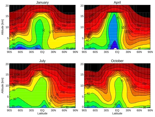
Figure 2 shows zonally averaged O₃ concentrations for January, April, July and October. At the equator the air at all heights is characterized by relatively low O3,

as a result of convective transport of O3-poor air from the surface up to the tropical

tropopause. At higher latitudes, downward transport of O₃-rich air dominates. The 5

northern-hemispheric stratosphere/troposphere exchange (STE) is strong in April while the O3concentration is low in the tropical region reflecting stronger upwards transport.

In the southern hemisphere, STE maximizes in austral spring. Photochemical produc-tion of O3is strongest in summer in the NH and convection leads to efficient transport

of O3precursors out of the boundary layer and mixing into the free troposphere.

10

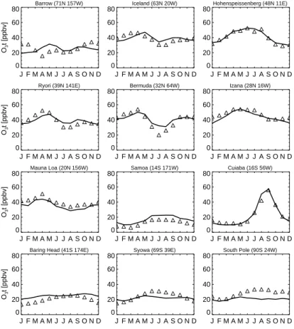
We have compared the baseline simulation with a wide range of long term obser-vations. Figure 3 shows the simulated and observed monthly mean O3

concentra-tions near the surface. The observational data are from the World Data Centre for Surface Ozone (WDSO) (http://gaw.kishou.go.jp/wdcgg.html), with major contributions from CMDL. We have selected stations with data covering the years 1996–2004 where 15

possible. The ozone concentrations from the simulation are averaged over 1996– 2005. Most of the observations are well reproduced by the model. For the northern-hemisphere extratropical remote sites, the observations are characterized by a spring maximum and a summer minimum associated with relatively strong downward flux of O₃from the stratosphere in the spring and efficient photochemical destruction in sum-20

mer. A summer maximum over polluted continental areas (e.g. at Hohenpeissenberg) associated with intensified photochemical production is well reproduced by the model. There are some discrepancies between the model and the measurements. At Bar-row, the observed spring minimum in surface O3may well be associated with bromine

chemistry (Barrie et al., 1988) which is not represented in the model. The observed 25

summer minima at Ryori and Bermuda are weak in the model simulation. At the south-ern tropical sites, the observations indicate an austral spring maximum which is well captured by the model. The year-round low O3value in Samoa is well simulated. The

(13)

ACPD

7, 11141–11189, 2007

Full Screen / Esc

EGU

reproduced. The observed surface O₃ concentrations at southern middle and high latitudes shows a winter maximum and a summer minimum in the lower troposphere. This feature is not well simulated by the model. The seasonal cycle produced by the model is relatively weak and does not reflect that of the measurements. The model over-estimates summer O3concentrations in Baring Head and also underestimates O3

5

values by up to 20 ppbv in the austral winter-spring over Antarctica. The cause of these discrepancies needs to be investigated further.

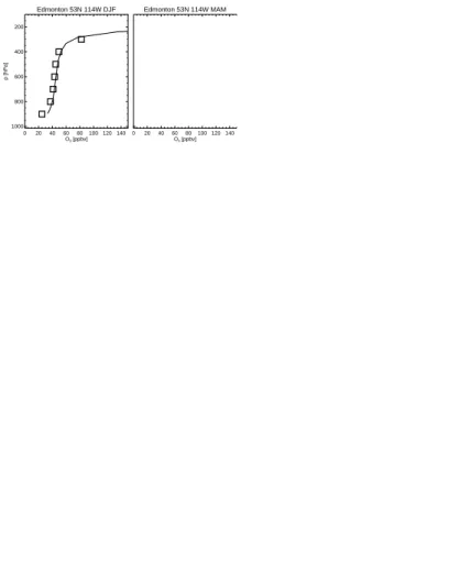
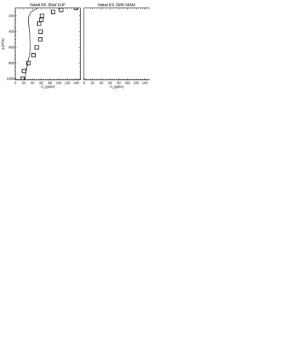
We have also compared the modelled vertical ozone concentrations to O3 sonde

measurements (Logan, 1999) made between 1985–1995 (Fig. 4). Note that the ozone concentrations from the baseline simulation are averaged over 1996–2005. The model 10

simulation agrees reasonably well with the observations. The model captures very well the strong vertical O3concentration gradient shown in the measurements in middle to

high latitudes in both hemispheres. However, the model overestimates spring-summer mid-upper tropospheric O₃concentrations to some degree (e.g. at Edmonton). The mid tropospheric maxima in the northern subtropical sites at Kagoshima and Hilo are well 15

simulated by the model. In the southern tropical sites at Natal and Samoa, the model simulates the steep decrease of O₃concentrations in the lower troposphere but cannot reproduce well the elevated O3 concentrations in the middle and upper troposphere,

especially in Natal, indicating possibly that there is not enough convective lifting of O3

and its precursors to the middle and upper troposphere during the biomass burning 20

season.

In general the model does a good job in simulating observed O3. However, to

under-stand factors affecting O3it is necessary also to look at the processes involved in ozone

production, destruction and transport. The ozone budget depends critically on the con-centration of ozone precursors and comprises the chemical production and destruction 25

of O₃, stratosphere/troposphere exchange (STE) and dry deposition at the surface. Al-though models can generally reproduce the observations of O3 concentrations, there

are large differences in tropospheric O3 budgets between different models (see, e.g.,

(14)

ACPD

7, 11141–11189, 2007

Full Screen / Esc

EGU

net chemical production varies from –810 to 550 Tg/year; the flux from the strato-sphere to the tropostrato-sphere from 390 to 1440 Tg/year; and the dry deposition from 533 to 1237 Tg/year. Most recent intermodel comparison shows that differences in O3

bud-get caculations are reduced among models for the present-day scenario (see Steven-son et al., 2006). In our calculations (see Table 3 − scenario A), the net influx from the 5

stratosphere is 452 Tg/year which is within the range reported by Houghton (2001) and Stevenson et al. (2006). The main chemical reactions contributing to O₃production are reactions between NO and hydroxyl peroxide/other peroxyl radicals (RO2). The

chem-ical destruction channels are mainly through the reactions H2O+O( 1

D) and O3+HOx.

The net chemical production (NCP) of 512 Tg/year calculated from these main terms 10

is within the reported range. Note that it is a small residual of two large production and destruction terms which are 3620 to 3108 Tg/year, respectively, in our calculation. Gross ozone production vary greatly across models on present-day simulations (2300 to 5300 Tg/year) (Stevenson et al., 2006) and are likely due to differences in complex-ities of chemical mechanisms included (see also discussions by Wu et al., 2007). Our 15

dry deposition of 1035 Tg/year is at the high end of the model range. The total tropo-spheric burden of 314 Tg is within the range seen in other models. We use a 150 ppbv O3 threshold to define tropospheric air. All the budget calculations are the global sum

below this threshold. 4.2 Nitrogen species 20

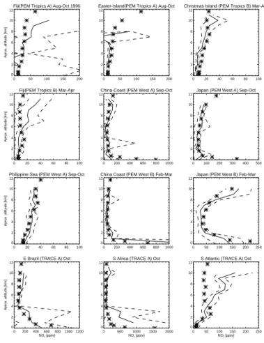
The model calculated NO₂ column averaged for year 2000 is in good agreement with the GOME measurement (not shown). Here we emphasize speciated comparisons; we compare some measured and modelled NOx and PAN vertical profiles. The

observa-tion data are from short-term aircraft campaigns compiled by Emmons et al. (2000) and should not necessarily compare in detail with model results from a climate simulation. 25

Nevertheless, the modelled NOxconcentrations are generally in reasonable agreement

with observations especially in the mid troposphere (see Fig. 5). The low NOx

(15)

ACPD

7, 11141–11189, 2007

Full Screen / Esc

EGU

The model does a good job in reproducing higher NO_x mixing ratios in the lower tro-posphere during February-March (PEM-West-B) in East Asia, arising from the strong influence of local anthropogenic emissions. Note, in particular, that the “C” shaped profile found in observation along the Japanese coast is well simulated by the model. Biomass burning in Africa and South America during September-November (TRACE-5

A) leads to a large near-surface enhancement of NOxmixing ratios in the surrounding

regions. The NO_xprofile in East Brazil is well reproduced but the model underestimates NOx mixing ratios in the lower troposphere in South Africa during the biomass

burn-ing season. The higher mixburn-ing ratios of NOx seen in the middle to upper tropospheric

over the South Atlantic during September-November are from biomass burning emis-10

sions that have been transported from the continents (PEM-Tropics-A and Tracer-A) (see Emmons et al., 2000 and references therein); this is not reproduced by the model. Note that the modelled data are the average over a decade; hence they do not capture interannual variability of emissions (which are the same for every year of the model run) and meterological conditions. Savage et al. (2007)2 have recently pointed to the 15

importance of interannual variations in meteorology for explaining observed NOx.

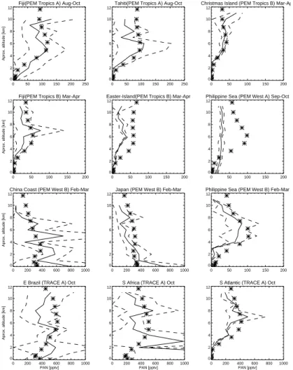
A comparison of modelled and observed PAN is shown in Fig. 6. Modelled PAN depends strongly on the magnitude of the VOC and NOx emissions sources and the

regional meteorology, as well as on the precise hydrocarbon degradation scheme in-cluded. With isoprene chemistry in this version of the model, modelled PAN has been 20

improved considerably compared to the previous version without isoprene chemistry which systematically underestimated PAN (not shown). The model simulates well the increase of PAN with altitude over the oceans. The peak observed in the Pacific and Atlantic oceans in the 4–8 km region during PEM-Tropics-A and Tracer-A, associated with the transport of PAN from South America, Australia and Africa, is reproduced by 25

the model. PAN profiles over the China Coast and Japan observed during PEM West B reflect strong outflow of pollutants from Asia to the North Pacific with high values

2

Savage, N. S., Pyle, J. A., Braesicke, P., et al.: The sensitivity of NO₂columns to interannual

(16)

ACPD

7, 11141–11189, 2007

Full Screen / Esc

EGU

seen near the surface; the model simulates this feature well. PAN over the Philippine Sea peaks in the middle troposphere reflecting the transport of PAN from the Asian continent (PEM West B). However, the seasonal change of PAN over the Philippine sea is not well captured by the model. High levels of PAN observed during September-November (TRACE A) are the result of biomass burning in Africa and South America 5

and the transport to the South Atlantic ocean. The model well simulates the vertical profiles of PAN in these regions. Addition of isoprene to the model has led to a much improved NO_y distribution compared with our earlier model simulations.

5 Tropospheric composition changes between 2000 and 2100

5.1 Response to anthropogenic emission changes 10

Figure 7 shows calculated changes in surface O3 for January and July between 2000

and 2100 assuming only changes in emissions (i.e. Run B–Run A). In the Northern Hemisphere, increases of O₃peaking above 40 ppbv are calculated over the polluted continents, with the largest increase of O3 in the Far East in summer. The areas

of larger ozone increase are regions where rapid economic growth and population in-15

crease are predicted. In January, there are significant increases of O₃over the oceans. For the Pacific region this corresponds to an outflow of pollutants from Asia, highlight-ing the potential importance of the Asian plume and its impact on global O3 levels in

the future. In the Southern Hemisphere, O₃ increases of 30 ppbv are calculated in South Africa and South America. The long range transport of O3from these regions is

20

evident: There is a background O3increase of up to 5–15 ppbv in the southern

hemi-sphere in remote oceanic areas. Increased surface emissions of O₃ precursors not only contribute to O3 formation in the source region (air quality) but also increase the

O3level in remote regions through long-range transport.

Figure 8a shows the calculated zonally averaged O₃ changes between 2000 and 25

(17)

ACPD

7, 11141–11189, 2007

Full Screen / Esc

EGU

free troposphere; it is a consequence of increases in emissions in northern latitudes and weak destruction of O₃ above the boundary layer. The O₃ increase in the strato-sphere results from transport of O3 precursors from the troposphere, although the

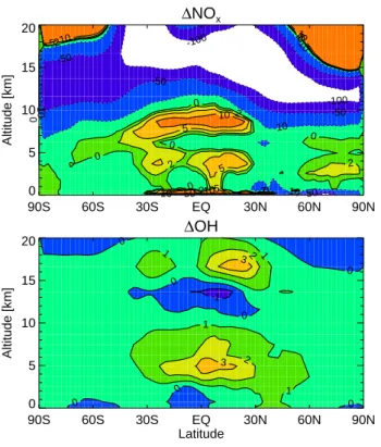
in-crease is relatively small compared to the background. Figure 8b shows NOxchanges

for B-A; largest increases are in the boundary layer where the direct emissions occur, 5

and in the upper tropical troposphere where its lifetime is long. There, large increases of NOx result in substantial O3production.

The global tropospheric O₃ budgets for scenario B are shown in Table 3. The net stratospheric influx is about 5% smaller than in scenario A. This small net decrease is the result of a larger tropical troposphere-to-stratosphere O3 flux in B that more than

10

offsets the middle latitude O3 influx from the stratosphere. Chemical production

in-creases substantially as a result of increasing emissions of O3 precursors. Chemical

destruction also increases in response to the increased O3. The overall net chemical

production of O₃ is nearly three times that of scenario A. With higher O₃, the dry de-position increases by a factor of 1.7. The average tropospheric O3 burden increases

15

from 314 to 549 Tg.

OH controls the oxidizing capacity in the troposphere and its distribution depends critically on NOxand hydrocarbons. Increases of NOxand O3tend to increase OH and

increases of CO and CH4 depress OH. Figure 8c shows changes in OH in response

to changes in NO_x/VOCs emissions; there are increases throughout the tropical tro-20

posphere with the largest increase in the upper troposphere, corresponding to the increase of NOx there. OH decreases in a large area of the NH and some of the SH

as a result of increases of VOCs over the continents. Although the tropospheric OH burden increases by 17% from run A to run B, the methane lifetime decreases only slightly from 11.3 to 11.2 years (see Table 3); the methane lifetime is mainly influenced 25

(18)

ACPD

7, 11141–11189, 2007

Full Screen / Esc

EGU

5.2 Response to climate change

The impact of climate change on the O3 distribution and its budget is assessed by

considering the differences between run C and run B, where only differences arise from the doubling CO₂(see Table 1). Figure 9 shows the differences in temperatures caused by a doubled CO2forcing. The average temperature increase is 2–3 K at the

5

surface (higher at high latitudes) and reaches 9K in the upper tropical troposphere. Cooling in the lower stratosphere occurs in the double-CO₂climate. Specific humidity increases throughout the troposphere with substantial increase in the tropical boundary layer by 20% (not shown).

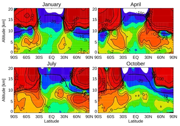
Figure 10 shows zonal mean changes of O₃ due to climate change for January, 10

April, July and October. It shows that for all seasons enhanced chemical destruction, due to increased water vapour in the projected future climate, dominate O3 changes

in the tropical troposphere. A pronounced feedback is the substantial increase of O₃ (over 200 ppbv) in the extratropical low stratosphere which is a response to changes in circulation; the enhanced Brewer-Dobson circulation more rapidly lifts O3-poor air

15

upwards in the tropics and transports O₃-rich air into high latitudes. This leads to an O3 reduction in the upper tropical troposphere and an O3 buildup at high latitudes in

the lower stratosphere, (in part also due to reduced ozone destruction in the cooler lower stratosphere, consistent with our earlier finding based on an older model version (Zeng and Pyle, 2003)). In a recent multimodel comparison (Butchart et al., 2006) 20

most participating models also produce an increase in the stratosphere-troposphere mass exchange rate in response to growing greenhouse gas concentrations. Conse-quently, the enhanced STE transports stratospheric O₃more rapidly to the troposphere leading to significant increases of O3 in the free troposphere; For the NH this feature

is most pronounced in April, shown in Fig. 10b when STE normally maximizes. The 25

influence of STE peaks in Austral winter/spring for the SH, leading to increased O₃ in the free troposphere which also propagates to the lower troposphere. The elevated O3 levels over the southern midlatitudes and the Antarctic in July and October shown

(19)

ACPD

7, 11141–11189, 2007

Full Screen / Esc

EGU

in Figure 10c,d seems linked due to increased stratosphere to troposphere transport of O₃and low surface O₃deposition rates at these locations (namely water and snow surfaces). Note that the decreases of O3along the tropopause are due to tropopause

lifting in a changed climate.

Responses of ground-level O₃ to climate change are highly complex. Figure 11 5

shows monthly mean surface O3 changes for January, April, July and October, in

response to a doubling of CO2. O3 changes are predominately negative through

increased water vapour for all the seasons, with the largest decrease over tropical oceans. However, we note some prominent, seasonally-varying O3 increases, e.g.,

over some of the polar regions, over the Southern Ocean in Austral winter, and over 10

some of the continents, with largest increases over Amazonia, Africa, North America, southern and central Europe in summer. The significant increase of O3over the Arctic

in April shown in Fig. 11b (most pronounced in February/March, not shown) may be due to an intensified poleward transport of O₃/O₃ precursors from North America and Eu-rope, possibly associated with increased STE, but needs further investigation. There is 15

also some increase of O3over the Arctic in October following summer increases of

sur-face O₃over Europe and North America. We also note that, to some extent, increases of surface O3 are linked to increased surface temperatures. A number of mechanisms

can lead to increased O3production following increased temperature: 1) favoured

pro-duction of HOxdue to mostly positive temperature-dependencies of CH4/VOC oxidation

20

reaction rate constant which fuel ozone formation; our calculations show that increases of HOx correlate closely to the increase in O3, and 2) the faster decomposition of PAN

which releases NO2 leading to regionally increase of ozone production, especially in

the NH polluted regions. Over Amazonia, southern Africa and southern Europe the model predicts a reduced humidity following the increased temperaure associated with 25

reduced soil moisture (Cox et al., 2004), reducing the O3destruction in those regions.

The climate change also comprises changes of convection, which play an important role in redistributing O3 and its precursors in the troposphere (see Lawrence et al.

(20)

ACPD

7, 11141–11189, 2007

Full Screen / Esc

EGU

NO_xoccur mainly in the tropical upper and middle troposphere, which are likely due to increased deep convection and the increased lightning activity respectively. Enhanced convection can transport NOxand other O3precursors to the upper troposphere more

efficiently, while intensified lightning produces NOx directly in the free troposphere,

leading to increased O3 chemical production in the free troposphere. On the other

5

hand, increased convection could bring O3-poor air (e.g. from the Pacific “warm pool”)

to the upper troposphere which contributes to O₃ decreases there. The O₃increases at 5–10 km over the tropics in July and into October shown in Fig. 10 are most likely associated with increased convection/lightning. Note that the large negative changes of NO_x above 10 km are partly due to strengthened circulation associated with the 10

double-CO₂climate forcing, and in part due to increased formation of HNO₃from NO_x in extratropical latitudes, favoured by the lower temperatures.

In a future climate the OH concentration will be modified following the increase of wa-ter vapour, which can subsequently modify the oxidizing capacity of the atmosphere. Responding to a double-CO2 climate, increases of OH occur throughout the

tropo-15

sphere (Fig. 12b) with an important feedback on the methane lifetime. Methane is an important greenhouse gas and is also a key trace gas controlling background O₃ con-centrations. In these calculations the methane lifetime has shortened considerably (by 1.8 years) in response to the double-CO2 forcing, due not only to increased OH

con-centrations but also to the increased reaction rate coefficient of OH+CH4which has a

20

strongly positive temperature-dependence.

Impacts of the climate change on the chemical and dynamical processes that affect tropospheric O₃ are reflected in the O₃ budget. Budget calculations (Table 3) show that with climate change included, the tropospheric O3 burden reduces slightly, as a

result of several competing processes. The most significant positive feedback is a 80% 25

increase of net flux of O₃ from the stratosphere to the troposphere. Both chemical production and destruction show increases under the climate change. The largest negative chemical change is through reaction O(1D)+H2O following photolysis of O3.

(21)

ACPD

7, 11141–11189, 2007

Full Screen / Esc

EGU

(by 4.5%) and NO+CH3O2(by 13%), which lead to O3production. We note the larger

relative increase in NO+CH3O2; the driving factor is the strong positive

temperature-dependence of the methane oxidation by OH which favours CH3O2production at higher

temperatures (Recall that CH₄ concentrations are fixed at the same value for runs B and C). Higher CH4levels could have a significant impact on tropospheric O3in a future

5

warmer climate. Finally, note that enhanced convection is reflected in a 26% increase of lightning-NO_xemission.

We have shown here that climate change has diverse impacts on O3 production,

loss and transport, and that the oxidizing capacity of the troposphere is modified by climate change. The feedbacks of climate change on tropospheric ozone are complex. 10

In particular, changes of surface O₃in response to climate change vary regionally and seasonally. More studies are needed to address in detail, for example, how changes in transport patterns can affect surface O3changes.

5.3 Response to climate change induced natural emission changes 5.3.1 Increased isoprene emissions

15

Relatively to scenario C, we increase isoprene emissions by 50% globally to assess the possible impact on O3. Note that the major emission regions are in the tropics in

the maritime continent, in South America and Africa. The Southeast USA is a region-ally important extra tropical source. Our calculation shows that increasing isoprene emissions has little impact on the global tropospheric ozone burden, which decreases 20

by less than 1% (see Table 3). However, the spatial distribution of ozone is modified; Fig. 13a shows that ozone generally increases in the northern hemisphere throughout the model domain and decreases in the equatorial and southern subtropical regions. The largest negative change of O3 occurs between 5–10 km in the southern tropics

where NOx concentrations are low. Budget calculations (see Table 3) show that with

25

extra isoprene emissions, the gross chemical production is reduced slightly due to a reduced NOx level which is consumed by elevated RO2 radicals from isoprene

(22)

oxida-ACPD

7, 11141–11189, 2007

Full Screen / Esc

EGU

tion to form PAN. O₃loss increases due to increased destruction by reactions with HO₂ and isoprene, respectively. Following the reduced OH level, the global methane lifetime increases by 0.6 years.

The largest impact of the increased isoprene emissions occurs in summer. Fig. 14a shows O3 changes at the surface for July; O3 generally decreases over the isoprene

5

source regions where NOx levels are also low, as a result of ozone destruction (less

O₃ production) in the NO_x-limited regime. In high NO_x regions (Europe and Asia), O₃ increases by up to 4–6 ppbv due to increased peroxy radicals from the degradation of isoprene which contribute positively to ozone production in the NOx-rich (VOC-limited)

environment. We also find elevated ozone concentrations away from the main emitting 10

sources (e.g. over the North Atlantic and western Africa). This suggests that PAN plays an important role in ozone formation; PAN can transport NOxaway from its source and

contribute to ozone production in remote regions. In our simulation background O3

concentrations has increased by around 1 ppbv except over the southern oceans. We will consider a range of future isoprene scenarios in more detail (Young et al., 20071; 15

Young, 2007).

Of course, the link between climate and isoprene emission is more complicated than the simple scaling up of the emissions in this sensitivity experiment. Besides the effect of temperature, the magnitude and spatial distribution of isoprene emission is highly dependent on the plant species. Thus, any future natural or anthropogenic land use 20

change, such as the drying of the Amazon rain forest (Cox et al., 2004) or increase in crop growth, would have a large impact on the isoprene emission field. Furthermore, increases in atmospheric CO₂ may well decrease isoprene emission (Rosensteil et al., 2003; Arneth et al., 2007). Other climate-related factors such as water availability, changes in the flux of photosynthetically active radiation (PAR), nutrient delivery and 25

air pollution, will also effect isoprene and other biogenic emissions, either directly or through their impact on primary productivity.

(23)

ACPD

7, 11141–11189, 2007

Full Screen / Esc

EGU

5.3.2 Increased soil-NO_xemissions

We double the soil-NOx emission globally in this experiment and compare run E to

run C to assess the impact associated with increasing soil-NO_x emissions. The major emissions regions are the tropics and subtropics with the strongest sources from agri-culture, grassland, and tropical rain forests. Results show that increased soil NOx has

5

a substantial positive feedback on tropospheric ozone (3% increase of the tropospheric burden, see Table 3). Both gross chemical production and net chemical production in-crease compared to run C, which is driven by inin-creased NOxlevels. Figure 13b shows

that changes in zonal mean O₃are positive globally with a peak in the southern sub-tropics. Increases of O3 at the surface are largely in the source region but are also

10

due to transport to remote regions through long-range transport (Fig. 14b). This indi-cates that emission changes in the tropics have a significant impact on O₃ formation. O3 precursors are subjected to faster transport and are more chemically active in that

region.

These calculations of the effects of natural emissions on O3are very simple and the

15

results are merely indicative of possible impacts. However the impacts are potentially significant, and more detailed studies are needed to project future changes of natural emissions which can be included in models.

6 Conclusions

We have evaluated an updated tropospheric chemistry model which is incorporated into 20

a version of the UK Met Office climate model. The model is satisfactory in modelling present-day observed tropospheric ozone and nitrogen species. The ozone budget falls within reported ranges. We calculate a net stratospheric to tropospheric ozone flux of 452 Tg/year, a gross O₃ chemical production of 3620 Tg(O₃)/year, and a gross O₃ chemical destruction of 3108 Tg/year. However, the gross chemical production of 25

(24)

ACPD

7, 11141–11189, 2007

Full Screen / Esc

EGU

Calculations for a series of 2100 scenarios suggest that projected significant in-crease of anthropogenic emissions of ozone precursors could contribute to large ozone increases throughout the troposphere. A pessimistic (large emissions) scenario (SEES A2) leads to an unacceptable increases of surface ozone. Such that these would be significant exceedences of suggested health-related thresholds. An assessment of the 5

impact of climate change on global tropospheric ozone reveals a number of important feedbacks. Increased water vapour leads to increased O₃ destruction in the tropics, whereas enhanced stratosphere-troposphere exchange increases the net O3 flux to

the troposphere. The O3 changes at the surface in a future climate are complex and

regionally varying, and are strongly influenced by changes in temperature, humidity, 10

STE, and hemispheric transport patterns. We pay attention to some positive changes: in particular, we find elevated O3 over polluted continents especially during summer

months; increase of background O3over the Southern Ocean and the Antarctic during

austral winter/spring; and intensified poleward transport of pollutants from Europe and North America leading to elevated O3 in the Arctic, in particular during winter/spring.

15

Recent studies of the response of tropospheric O3 to climate change reveal diverse

model responses (Shindell et al., 2006; Brasseur et al., 2006). Multi-model studies are important to achieve a consensus on the impact of future climate change on tropo-spheric O3, in particular at ground-level.

Changes in convection in a double CO₂climate can modify the NO_xdistribution; En-20

hanced convection lifts NOx and other ozone precursors more efficiently in the tropical

region which contribute positively to the O3chemical production through elevated NOx

and HO_x in that region. The associated change in lightning-produced NO_x is approx-imately a 22% increase in our calculation and contributes positively to tropospheric ozone formation. However, the effect of the convection on ozone budgets are still un-25

certain (Doherty et al., 2005) and further studies are needed to quantify to what extent the tropospheric ozone budget is influenced.

Climate change modifies the tropospheric oxidizing capacity considerably. The methane lifetime is shortened by 1.8 years when climate change is included in the

(25)

ACPD

7, 11141–11189, 2007

Full Screen / Esc

EGU

calculation, due to increased OH concentrations in a more humid climate. In contrast, the methane lifetime was not changed significantly in run B which considered just the increases of anthropogenic emissions. In a warmer and wetter climate, methane can play a significant role in ozone formation due to the strong positive temperature depen-dence of its oxidation rate coefficient. Further studies are needed to assess the role of 5

methane on ozone formation, particularly in a changed climate.

In addition to considering changing anthropogenic emissions in the 2100 climate change experiment, we have also examined idealised changes of some natural emis-sions and their impact on tropospheric ozone. With a 50% increase of the isoprene emission, changes in surface ozone range from –8 ppbv to 6 ppbv. The impacts are 10

regionally varying and have a relatively strong seasonal cycle. The largest decreases of surface ozone occur over isoprene source regions (Amazonia, US, Africa and South East Asia) and the largest increases are over China and Europe in summer where NOx

levels are high. Generally the response to changed isoprene depends on whether the chemical regime is NOx- or VOC-limited: so we predict zonal mean ozone decrease in

15

the southern hemisphere and tropics, with ozone increases in the north hemisphere. The increased isoprene emission increases methane lifetime by 0.6 years, which is large compared with changing anthropogenic emissions. By doubling soil-NOx

emis-sions, we obtain substantial increases of ozone over emitting regions and a 0.4 years reduction on methane lifetime. Changes in biogenic emissions, which are mainly from 20

tropics and subtropics, can significantly affect the oxidizing capacity of the troposphere. More study is needed to reduce the uncertainty in present estimates of natural emis-sions. Accurate projections of the future biogenic emissions are crucial to assessing chemistry-climate-biosphere feedbacks.

Acknowledgements. This work is funded by the NERC National Centre for Atmospheric

Sci-25

ence (NCAS). The anthropogenic emission data are made available by the ACCENT commu-nity. Hadley Centre is thanked for the use of the UM. P. J. Young is funded by NERC through a studentship with a CASE award from the UKMO.

(26)

ACPD

7, 11141–11189, 2007

Full Screen / Esc

EGU References

Arneth, A., Niinemets, U., Pressley, S., et al.: Process-based estimates of terrestrial ecosystem isoprene emissions, Atmos. Chem. Phys., 7, 31–53, 2007,

http://www.atmos-chem-phys.net/7/31/2007/.

Atkinson, R., Baulch, D. L., Cox, R. A., Hampson, R. F., Kerr, J. A., Rossi, M. J., and Troe, J.:

5

Evaluated kinetic and photochemical data for atmospheric chemistry, organic species:

Sup-plement VII, J. Phys. Chem. Ref. Data, 28(2), 191–393, 1999. 11147

Barrie, L. A., Bottenheim, J. W., Schell, R. C., Crutzen, P. J., and Rasmussen, R. A.: Ozone destruction and photochemical reactions at polar sunrise in the lower Arctic atmosphere, Nature, 334, 138–140, 1988.

10

Berntsen, T. K., Myhre, G., Stordal, F., and Isaksen, I. S. A.: Time evolution of tropospheric

ozone and its radiative forcing, J. Geophys. Res., 105, 8915–8930, 2000. 11144

Brasseur, G., Kiehl, J. T., M ¨uller, J.-F., Schneider, T., Granier, C., Tie, X., and Hauglustaine, D.: Past and future changes in global tropospheric ozone: Impact on radiative forcing, Geophys.

Res. Lett., 25, 3807–3810, 1998. 11144

15

Brasseur, G. P., Schultz, M., Granier, C., Saunois, M., Diehl, T., Botzet, M., Roeckner, E., and Walters, S.: Impact of climate change on the future chemical composition of the global troposphere, J. Clim., 19, 3932–3951, 2006.

Butchart, N., Scaife, A. A., Bourqui, M., et al.: Simulations of anthropogenic change in the strength of the Brewer-Dobson circulation, Clim. Dynam. 27, 727–741, 2006.

20

Carver, G. D. and Stott, P. A.: IMPACT: An implicit time integration scheme for chemical species and families, Ann. Geophys., 18, 337–346, 2000,

http://www.ann-geophys.net/18/337/2000/. 11147

Collins, W. J., Derwent, R. G., Garnier, B., Johnson, C. E., Sanderson, M. G., and Stevenson, D. S.: The effect of stratosphere-troposphere exchange on the future tropospheric ozone

25

trend, J. Geophys. Res., 108, 8528, doi:10.1029/2002JD002617, 2003. 11144

Cox, P. M., Betts, R. A., Collins, M., Harris, P. P., Huntingford, C, and Jones, C. D.: Amazo-nian forest dieback under climate-carbon cycle projections for the 21st Century, Theor. Appl. Climatol., 78, 137–156, 2004.

Cullen, M. J. P.: The unified forecast/climate model, Meteorol. Mag., 122, 81–94, 1993. 11146

30

DeMore, W. B., Sander, S. P., Golden, D. M., Hampson, R. F., Kurylo, M. J., Howard, C. J., Rav-ishankara, A. R., Kolb, C. E., and Molina, M. J.: Chemical kinetics and photochemical data

(27)

ACPD

7, 11141–11189, 2007

Full Screen / Esc

EGU

for use in stratospheric modeling, evaluation number 12: NASA panel for data evaluation,

JPL Pub. 97-4, 1997.11147

Dentener, F., Stevenson, D., Cofala, J., Mechier, R., Amann, M., Bergamaschi, P., Raes, F., and Derwent, R.: The impact of air pollutant and methane emission controls on tropospheric ozone and radiative forcing: CTM calculations for the period 1990-2030, Atmos. Chem.

5

Phys., 5, 1731–1755, 2005,

http://www.atmos-chem-phys.net/5/1731/2005/. 11149

Doherty, R. M., Stevenson, D. S., Collins, W. J., and Sanderson, M. G.: Influence of convective transport on tropospheric ozone and its precursors in a chemistry-climate model, Atmos. Chem. Phys., 5, 205–3218, 2005,

10

http://www.atmos-chem-phys.net/5/205/2005/.

Edwards, J. M. and Slingo, A.: Studies with a flexible new radiation code. I: Choosing a

config-uration for a large-scale model, Q. J. Roy. Meteor. Soc., 122, 689–719, 1996. 11147

Emmons, L. K., Hauglustaine, D. A., M ¨uller, J.-F., Carroll, M. A., Brasseur, G. P., Brunner, D., Staehelin, J., Thouret, V., and Marenco, A.: Data composites of airborne observations of

15

tropospheric ozone and its precursors, J. Geophys. Res., 105(D16), 20 497–20 538, 2000. Forster, P. M. F., Johnson, C. E., Law, K. S., Pyle, J. A., and Shine, K. P.: Further estimates

of radiative forcing due to tropospheric ozone, Geophys. Res. Lett., 23, 3321–3324, 1996.

11144

Giannakopoulos, C., Chipperfield, M. P., Law, K. S., and Pyle, J. A.: Validation and

intercom-20

parison of wet and dry deposition schemes using210Pb in a global three-dimensional off-line

chemical transport model, J. Geophys. Res., 104, 23 761–23 784, 1999.11148

Gregory, D. and Rowntree, P. R.: A mass flux convection scheme with representation of cloud ensemble characteristics and stability dependent closure, Mon. Weather Rev., 118, 1483–

1506, 1990. 11147

25

Grenfell, J. L., Shindell, D. T., Koch, D., and Rind, D.: Chemistry-climate interactions in the Goddard Institute for Space Studies general circulation model 2. New insights into modeling

the preindustrial atmosphere, J. Geophys. Res., 106, 33 435–33 451, 2001.11144

Guenther, A., Hewitt, C. N., Erickson, D., et al.: A global model of natural volatile

organic-compound emissions, J. Geophys. Res., 100, 8873–8892, 1995.11145,11149

30

Hauglustaine, D. A., Granier, C., Brasseur, G. P., and M ´egie, G.: The importance of atmospheric chemistry in the calculation of radiative forcing on the climate system, J. Geophys. Res., 99,

(28)

ACPD

7, 11141–11189, 2007

Full Screen / Esc

EGU

Hauglustaine, D. A. and Brasseur, G. P.: Evolution of tropospheric ozone under anthropogenic activities and associated radiative forcing of climate, J. Geophys. Res., 106, 32 337–32 360, 2001 11144

Hauglustaine, D. A., Lathiere, J., Szopa, S., and Folberth, G. A.: Future tropospheric ozone simulated with a climate-chemistry-biosphere model, Geophys. Res. Lett., 32, L24807,

5

doi:10.1029/2005GL024031, 2005. 11145

Houghton, J. T., Ding, Y., Griggs, D. J., Noguer, M., van der Linden, P. J., Dai, X., Maskell, K., and Johnson, C. A. (Eds.): Climate Change 2001: The Scientific Basis, Cambridge Univ.

Press, Cambridge, UK, 2001. 11143

Johns, T. C., Gregory, J. M., Ingram, W., J., et al.: Anthropogenic climate change for 1860 to

10

2100 simulated with the HadCM3 model under updated emissions scenarios, Clim. Dyn., 20,

583–612, 2003. 11146

Johnson, C. E., Collins, W. J., Stevenson, D. S., and Derwent, R. G.: Relative roles of climate and emissions changes on future tropospheric oxidant concentrations, J. Geophys, Res.,

104, 18 631–18 645, 1999. 11144

15

Lathiere, J., Hauglustaine, D. A., De Noblet-Ducoudre, N., Krinner, G., and Folberth, G. A.: Past and future changes in biogenic volatile organic compound emissions simulated with a global dynamic vegetation model. Geophys. Res. Lett., 32, L20818, doi:10.1029/2005GL024164,

2005. 11145

Law, K. S. and Pyle, J. A.: Modeling trace gas budgets in the troposphere, 1. Ozone and odd

20

nitrogen, J. Geophys. Res., 98, 18 377–18 400, 1993. 11147

Law, K. S., Plantevin, P. H., Shallcross, D. E., Rogers, H. L., Pyle, J. A., Grouhel, C., Thouret,

V., and Marenco, A.: Evaluation of modeled O₃ using Measurement of Ozone by Airbus

In-Service Aircraft (MOZAIC) data, J. Geophys, Res., 103, 25 721–25 737, 1998.11147

Lawrence, M. G., von Kuhlmann, R., Salzmann, M., and Rasch, P. J.: The balance of

ef-25

fects of deep convective mixing on tropospheric ozone, Geophys. Res. Lett., 30(18), 1940, doi:10.1029/2003GL017644, 2003,

Leonard, B. P., Lock, A. P., and MacVean, M. K.: The NIRVANX scheme applied to one-dimensional advection, Int. J. Numer. Methods for Heat and Fluid Flow, 5, 341–377, 1995.

11146 30

Li, D. and Shine, K. P.: A 4-D ozone climatology for UGAMP models, UGAMP internal report, 1995.

(29)

test-ACPD

7, 11141–11189, 2007

Full Screen / Esc

EGU

ing 3-D models and development of a grided climatology for tropospheric ozone, J. Geophys. Res., 104, 16 115–16 149, 1999.

Marenco, A., Gouget, H., N éd élec, P., Pag és, J.-P., and Karcher, F.: Evidence of a long-term in-crease in tropospheric ozone from Pic du Midi data series: Consequences: Positive radiative

forcing, J. Geophys. Res., 99, 16 617–16 632, 1994. 11143

5

Mickley, L. J., Murti, P. P., Jacob, D. J., Logan, J. A., Koch, D. M., and Rind, D.: Radiative forc-ing from tropospheric ozone calculated with a unified chemistry-climate model, J. Geophys.

Res., 104, 30 153–30 172, 1999. 11144

Monson, R. K. and Fall R.: Isoprene emission from aspen leaves: Influence of the environ-ment and relation to photosynthesis and phptorespiration, Plant Physiol., 90, 267–274, 1989.

10

11145

Naki´cenovi´c, N., Alcamo, J., Davis, G., et al.: Special Report on Emission Scenarios,

Cam-bridge Univ. Press, CamCam-bridge, UK, 599, 2000. 11149

Olivier, J. G. J., and Berdowski, J. J. M.: Global emissions sources and sinks, in The Climate System, edited by Berdowski, J., Guicherit, R., and Heij, B. J., pp. 33–78, A.A. Balkema

15

Publishers/Swets and Zeitlinger Publishers, Lisse, The Netherlands. ISBN-90-5809-255-0, 2001.

Pegoraro, E., Rey, A., Barron-Gafford, G., Monson, R., Malhi, Y., and Murthy, R.: The interacting

effects of elevated atmospheric CO2concentration, drought and leaf-to-air vapour pressure

deficit on ecosystem isoprene fluxes, Oecologia, 146, 120–129, 2005. 11145

20

P ¨oschl, U., von Kuhlmann, R., Poisson, N., and Crutzen, P. J.: Development and intercom-parison of condensed isoprene oxidation mechanisms for global atmospheric modeling, J.

Atmos. Chem., 37(1), 29–52, 2000. 11147

Price, C. and Rind, D.: A simple lightning parameterization for calculating global lightning dis-tributions, J. Geophys. Res., 97, 9919–9933, 1992.

25

Price, C. and Rind, D.: Modelling global lightning distributions in a general circulation model, Mon. Weather Rev., 122, 1930–1939, 1994.

Roe, P. L.: Some contributions to the modelling of discontinuous flow, “Large-Scale Computa-tions in Fluid Mechanics”, edited by Engquist, B., Osher, S., and Somerville, R., American

Mathematical Society, Providence, Rhode Island.11146

30

Roelofs, G. J., Lelieveld, J., and van Dorland, R: A three-dimensional chemistry/general circula-tion model simulacircula-tion of anthropogenically derived ozone in the troposphere and its radiative