Geometry of integrable systems : from topological Lax systems to conformal field theories

(1)

HAL Id: tel-01878352

https://tel.archives-ouvertes.fr/tel-01878352 Submitted on 21 Sep 2018

HAL is a multi-disciplinary open access archive for the deposit and dissemination of sci-entific research documents, whether they are pub-lished or not. The documents may come from teaching and research institutions in France or abroad, or from public or private research centers.

L’archive ouverte pluridisciplinaire HAL, est destinée au dépôt et à la diffusion de documents scientifiques de niveau recherche, publiés ou non, émanant des établissements d’enseignement et de recherche français ou étrangers, des laboratoires publics ou privés.

systems to conformal field theories

Raphaël Belliard

To cite this version:

Raphaël Belliard. Geometry of integrable systems : from topological Lax systems to conformal field theories. Mathematical Physics [math-ph]. Université Pierre et Marie Curie - Paris VI, 2017. English. �NNT : 2017PA066175�. �tel-01878352�

(2)

Université Pierre et Marie Curie

ED564 - Physique en Ile-de-France

GEOMETRY OF INTEGRABLE

SYSTEMS

FROM TOPOLOGICAL LAX SYSTEMS TO CONFORMAL

FIELD THEORIES

Raphaël Belliard

1

PhD thesis under the supervision of Bertrand Eynard1,2 1 Institut de physique théorique, Université Paris Saclay,

CEA, CNRS, F-91191 Gif-sur-Yvette, France

2 Centre de recherches mathématiques, Université de Montréal, Canada

Reviewers

Lotte HOLLANDS Heriot-Watt University Sergei SHADRIN University of Amsterdam

Jury

Vasily PESTUN Institut des Hautes Etudes Scientiﬁques Claire VOISIN Collège de France

(3)

(4)

Figure 1: Real section of the complex surface of integrable quantizations, dispersionless limits and perturbative reconstruction.

(5)

(6)

(7)

(8)

“If a man does not keep pace with his companions, perhaps it is

because he hears a diﬀerent drummer. Let him step to the music which he hears however distant or far away.”

(9)

(10)

Abstract

This PhD thesis is about a framework in complex geometry and methods thereof for solving sets of compatible diﬀerential equations arising from integrable systems, classical or quantum, in the context of the geometry of

moduli spaces of connections over complex curves, or Riemann surfaces. It is based on the idea in mathematical Physics that integrable systems possess symmetries that impose algebro-diﬀerential constraints, so-called

loop equations, on the objects of interest (e.g. partition or correlation functions). In turn, we intend to solve these constraints recursively in certain topological regimes using a particular procedure called the topological recursion. Their solutions are in general generating functions

of enumerative-geometric quantities. Since they are for the most part determined by the initial data of the recursive process, it realizes in the

making an algebro-geometric classiﬁcation of the family of integrable models under consideration.

Résumé

Cette thèse de doctorat traîte d’un cadre en géométrie complexe et de méthodes pouvant y être développées pour résoudre des ensembles d’équations diﬀérentielles compatibles venant de systèmes intégrables, classiques ou quantiques, dans le contexte de la géométrie d’éspaces de modules de connexions au-dessus de courbes complexes, ou surfaces de Riemann. Elle vient de l’idée en physique mathématique que les symétries

des systèmes intégrables imposent aux objets d’intérêt (fonctions de partitions ou de corrélations) des contraintes algebro-diﬀérentielles nommées équations de boucles. Le but est par la suite de résoudre ces contraintes par récurrence dans des régimes dits topologiques en utilisant

une procédure nommée récurrence topologique. Leurs solutions sont en général les fonctions génératrices de quantités issues de problèmes de

géométrie énumérative. Etant principalement déterminées par les conditions initiales de la récurrence, on produit au passage une classiﬁcation algebro-géométrique de la famille de systèmes intégrables

(11)

Merci à vous !

Je remercie chaleureusement toutes les personnes qui m’ont accompa-gné, soutenu et aidé de quelque manière que ce soit lors du déroulement de cette thèse.

Tout d’abord sur le plan scientifique, je tiens tout particulèrement à remercier mon directeur de thèse Bertrand Eynard pour sa tolérance et l’excellente qualité de ses enseignements, j’en bénéficierai encore très longtemps et j’ai maintenant grâce à lui la capacité de discuter avec des chercheurs venant d’horizons très différents. Par la même ses anciens doc-torants, Nicolas Orantin, Olivier Marchal et Gae..tan Borot, qui ont au moins hérité de ces qualités. Je voudrais ensuite remercier l’ensemble de l’IPhT du CEA de Saclay pour m’avoir permis d’effectuer cette thèse dans de très bonnes conditions. En particulier, Sylvain Ribault pour de nom-breuses discussions très éclairantes ainsi que Didina Serban et Ivan Kostov pour m’avoir permis de participer à l’école d’été des Houches de 2016 sur les systèmes intégrables où j’ai autre autre suivi le cours de Joerg Teschner sur les théories conformes, une étape importante de ma thèse. J’y ai aussi rencontrè de nombreux amis et probables futurs collaborateurs. Je remer-cie aussi Boris Dubrovin pour m’avoir invité à passer un mois à la SISSA de Trieste, autre moment phare de mon projet. Je tiens ensuite à remercier les nombreux organisateurs d’écoles et de conférences qui m’ont permis voyager presque sans cesse et de tant apprendre.

Il n’y a pas de mots assez forts pour décrire le soutien inconditionnel que m’ont donné tous les membres de ma famille. Ma mère Abeba, mon frère Matthieu, ma sœur Mala..ιka, ma tante Sophie et chacun(e) des autres, de France, d’Italie et d’ailleurs, parmis lesquels je ne citerai que la relève, par ordre d’apparition, Sara, Claudia, Justine, Alo..ιs, Oscar, Lorenzo, Salomé, Martina, Federico, Louisiane, Miika, Maaza, Basile et Isla. Sans oublier ceux que je ne peux plus remercier.

(12)

Et enﬁn, pour ﬁnir, je remercie ceux qui me supportent au quotidien, tous les amis de cœur qui m’ont accueilli, rattrapé, calmé, motivé, lancé conseillé, aimé et que sais-je encore toutes ces dernières années.

(13)

(14)

Introduction

1 Integrability : a marriage

Theoretical Physics tries to give objective mathematical descriptions of not necessarily visible physical phenomena. To do so, it uses mathematical modeling to logically derive equations that measurable quantities of in-terest should satisfy. True objectivity not being possible to obtain, the theoretical approach would not have any meaning without its experimental counterpart. Statements or claims will then be called objectively true if they can be checked up to satisfying precisions in experimental devices. Its range of application is limitless and as such, it caused a lot of people to think that a theory of everything could be constructed. Unfortunately, simple reasoning gives a heuristic to the contrary. Indeed, a choice of the-oretical framework carries its own limits although whichever phenomenon we are trying to study will admit a description in terms of a mathematical model. Knowing what a model under consideration does not describe is of the utmost importance. A counterpart to this remark from logic theory can be found in the mathematician and logician Go..del’s completeness and incompleteness theorems that we will loosely state as

• Any theory admits a model.

• Any model admits an assertion that can neither be proved nor disproved That being written, we can at most hope for a theory describing objec-tively every phenomenon we know exists right now.

The equations arising from this method appear to be of various really diﬀerent natures. In particular, they can be exactly solvable, or integrable, namely one can give (an algorithm to compute) an expression of their

(19)

solutions, or not. If not, we have other ways to extract information from the model, from approximations and numerics to chaos theory. In this thesis we will study exclusively those problems that are integrable in this given sense.

One of the most important facts about exactly solvable equations aris-ing from theoretical Physics is that they are not at all the generic situation. Indeed as we shall see, they are those whose solutions satisfy many rela-tions. Intuitively, these relations enlarge the vocabulary at our disposition and this is what allows to formulate how to compute the corresponding solutions.

In the early XIXt h century, Liouville defined classical integrable systems as a subclass of models whose equations of motions are Hamiltonian flows on finite dimensional symplectic manifolds. They are those that possess

enough independent quantities that are conserved by the dynamics, enough

being half the dimension of the underlying space of states accessible to the system, namely the phase space. The reader can find all the needed definitions to understand these statements in the next chapter. This defin-ing theorem then shows that their equations of motions can be solved by means of algebraic operations and integrals (periods). Moreover, by use of so-called generating functions, these equations become those of uniform translations on invariant tori. We will generalize this notion of integra-bility throughout what follows. Moreover, in 1918, Nœther related smooth symmetries of the corresponding action to conserved quantities. These smooth symmetries are typically Lie group actions leaving the dynamics unchanged.

At this point one should note that in the past, all major advances in theoretical Physics were always achieved by using and developing contemporary Mathematics. The study of integrable systems explores this tight relationship in all its glory. Developing such theories requires some of the latest advances in virtually all ﬁelds of the mathematical uni-verse and gives rise to beautiful new structures among them. The reason is simple, the quest for objectivity that turned out to be so successful in Physics and the relative truth Mathematics provide are always compati-ble as being part of the same temporality and thus encompassing similar paradigm. An immediate consequence of this remark is that such

(20)

paral-1. INTEGRABILITY : A MARRIAGE vii lels can be made outside of those ﬁelds, with other sciences and arts. As mentioned, the core aim of the theoretical approach to Physics is to relate our reasoning and logical understanding to our perceptions, experiences and observations. The pre-Socratic Greek philosopher Protogoras deﬁned humanity as “the measure of all things”.

Topology, geometry and algebra are those parts of Mathematics that deal respectively with the notions of shapes, distances and angles, and mathematical symbols and the rules to manipulate them. In our way to use mathematical modeling, the objects that are considered in any one of these broad topics are interpreted in relation with the underlying Physics. In par-ticular, all the quantities one wishes to consider in a theory, ﬁxed constants of nature or not, can be treated as variables parameterizing deformations of the studied systems.

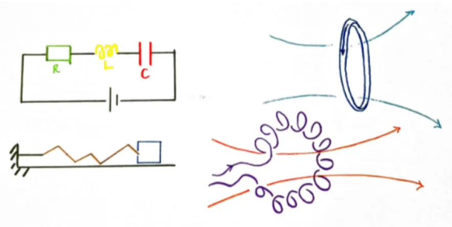
This brings us to the notion of deformation of theories, through the variations of their so-called moduli, namely their parameters. A natural question is then whether two given theories can be deformed one into the other in this sense. The answer is of course no in general. We know already however from elementary Physics textbooks some instances where this is the case. Let us mention two of those.

• the series RLC circuit is equivalent to the dissipative dynamics of a one dimensional spring, indeed they are both second order linear ﬁlters,

• incompressible vorticity in the hydrodynamics of smoke rings is equiv-alent to the magnetism of toroidal solenoids, indeed they both de-scribe rotational propagation of waves.

In addition, these are examples of integrable models, and as we shall see, the ability to switch from diﬀerent viewpoints using deformations of geometrical structures is a key feature of integrability.

In 1931, Bethe proposed an ansatz he used to solve exactly for accessi-ble states and their levels of energy in the so-called one-dimensional

anti-ferromagnetic Heisenberg model [24]. This is a problem treated quantum

mechanically to study critical points and phase transitions of certain mag-netic systems of spins. Thus was born the notion of quantum integrability.

(21)

Since then there has been a tremendous amount of work done to under-stand the geometry behind the algebraic structures whose presence allowed for exact solvability in quantum problems.

Figure 2: Elementary Physics correspondences.

In the last chapter of this thesis we will be interested in a particular type of quantum integrable system, namely conformal ﬁeld theory, possessing huge symmetry algebras. Let us therefore review some fundamentals of quantum Physics from an oriented geometric point of view, starting by a bit of history.

2 Quantum Physics and theory

At the dawn of the XXt h _{century, long after the industrial revolution, a} short list of problems stood apart from the seemingly global understand-ing of the world that had been oﬀered by thermodynamics and electro-magnetism. These unsolved problems had all been formulated during the previous century

• 1838 : Faraday discovers cathode rays

• 1860 : Kirchhoﬀ states the black-body radiation problem

• 1877 : Boltzmann suggests that the accessible energy levels of a system might be discrete

(22)

2. QUANTUM PHYSICS AND THEORY ix In 1900, Planck made the quantum hypothesis, stipulating that energy-radiating systems can be decomposed as fundamental energy blocks with energies proportional to the frequencies to which they respectively radiate. If we denote the energy of a building block by ² and its frequency by ν, this relation is written

² = hν, (2-1)

thus deﬁning the universal constant h ' 6.626.10−34_m2_kg_±s_{, called} Planck’s constant and measured since with great accuracy.

In 1905, as part of what has been called later the Annus Mirabilis papers of Einstein, he extended Planck’s hypothesis to light by introducing the photon, quantum of light, and explained in this way the photo-electric eﬀect.

• 1913 : Bohr quantizes the angular momentum of electrons in atoms • 1923 : de Broglie introduces matter-waves

• 1925 : Heisenberg, Born and Jordan develop matrix mechanics, Schro..dinger deﬁnes wave-mechanics and his famous equation as an approximation to de Broglie’s theory, Dirac writes his equation for the dynamics of electrons

• 1932 : von Neumann lays the rigorous mathematical basis for quantum mechanics as the theory of linear operators on Hilbert spaces

The quantum paradigm that came with these discoveries is a change of logic. Indeed, experiments such as Young’s experiment in 1801, that was generalized as the double slit experiment of Davisson and Germer in 1927, show that light and matter (with matter particles as big as the fullereneC60 whose molecule contains 60carbon atoms) behave sometimes as waves and

sometimes as particles, according to the observer. The quantum theory therefore redeﬁned the notions of observation and measure in the sense that it identiﬁed them as fundamental interactions. On one hand subparts of the system under consideration observe one another while on the second hand, the experimentalists are themselves an interacting part of the system.

(23)

Figure 3: Both energy and angular momentum levels are quantized in an atom.

By a quantum system we will from now on mean any collection of ob-jects, visible or not, that we may want to study from a quantum perspective. Rather than the usual cat of Schro..dinger’s thought experiment, let us consider human beings, part of a society where they can sometimes express their opinion through vote. At all time they may have several possibly contradictory opinions but the closer we get to the measure of that opinion the less multiple we appear, until the moment when a choice has to be made, choice from which we will have to evolve once again.

Quantum systems behave as voters : at all time in a superposition of states until one of these states is singled out by an observation or measurement.

As my dear friend Remi Jaoui once told me, we knew human beings were as such, we just had not realized matter as well. At least we had not taken it into account in the way we had tried to describe the world through Physics. Mystics from all around the globe and from as far back in time as one can imagine had already expressed this idea in their own words. The reason is probably that the European middle-age caused for a strong materialistic back-reaction that lasted around three hundred years in science and is still the predominant doctrine e.g. in economy or agriculture. In 1941, Feynman introduced the notion of path integral, a way of relating phenomena in quantum systems to their classical counterparts that tells us

(24)

2. QUANTUM PHYSICS AND THEORY xi that the outcome of a quantum event is an average over all the possible classical outcomes with respect to a (complexiﬁed) probability measure.

Let us brieﬂy and schematically describe this procedure. Let us denote by X the (possibly inﬁnite dimensional symplectic) phase space, or space of states accessible to a classical system. According to the principle of least

action, there exists a function

Scl : π01(X) −→ R

Γ 7−→ Scl[Γ] (2-2)

where π0

1(X) is the set of all possible trajectories in X, called the action functional and such that the classical trajectories followed by the system are those minimizing this action. They are in particular critical trajectories satisfying

δScl

δΓ = 0 (2-3)

Feynman’s method of the path integral is then to introduce the wave-function ψ :L_{−→ C} deﬁned on a Lagrangian subspace L_⊂X such that for any initial and ﬁnal states ϕi,ϕf ∈L, ψ is given in terms of an integral over all possible trajectories γ ⊂L, that is over one dimensional paths drawn on the space L, starting at ϕi and ending at ϕf, as

ψ(ϕi,ϕf) = d e f Z Γ∈π0 1(L) ∂Γ=ϕf −ϕi [DΓ]eiScl [Γ]ħ (2-4)

where we introduced Planck’s reduced constant ħ = ₂h_π and the

Boltzmann-type weight eiScl [Γ]ħ on the space of trajectories. The

wave-function written as such is not, in general, a well-deﬁned mathematical object but we will very soon see an alternative way to construct the physical quantities of interest. For the time being, let us consider these equalities as notations, a formal way to encode the algebraic properties the wave-function is assumed to have by deﬁnition.

(25)

We may not be willing to chose an initial and a final state for the system in which case we would define the so-called partition function by summing over all possible coinciding initial and final conditions.

Z = d e f Z L [Dϕ] Z Γ∈π0 1(L) ϕf =ϕi =ϕ [DΓ]eiScl [Γ]ħ (2-5) = Z Γ∈π1(L) [DΓ]eiScl [Γ]ħ (2-6)

Classically, physical quantities of interest, or observables, are functions

O :X_{−→ R}. In the quantum theory, their measure becomes uncertain and the previous construction allows to deﬁne their vacuum expected value at a state ϕ ∈L as O(ϕ)® = d e f 1 Z Z Γ∈π1(L) ϕ∈Γ [DΓ]eiScl [Γ]ħ O(ϕ) (2-7)

and similarly, for any integer n ∈ N∗, deﬁne the correlation of _n ob-servables O1, . . . ,On : X −→ R in the classical states ϕ1, . . . ,ϕn ∈ L by the formula O1(ϕ1) ···On(ϕn) ® = d e f 1 Z Z Γ∈π1(L) ϕ1,...,ϕn∈Γ [DΓ]eiScl [Γ]ħ O₁(ϕ₁) ···O_n(ϕ_n) (2-8)

Solving the theory then amounts to computing all such correlation func-tions between observables of interest. Let us now investigate a possible way for one to do so.

Assuming the Lagrangian L⊂X to be such that

|Scl[Γ]| −→ Γ→∂π1(L)

∞ (2-9)

when the trajectory Γ goes to the boundary ∂π1(L), yields

Z Γ∈π1(L) ϕ1,...,ϕn∈Γ [DΓ] δ δΓ ³ eiScl [Γ]ħ O₁(ϕ₁) ···O_n(ϕ_n) ´ = 0 (2-10)

(26)

3. CATEGORIFICATION AND TOPOLOGICAL STRING THEORY xiii for generic values of all the other arguments and using Leibniz rule, this can be rewritten as the so-called Schwinger-Dyson equations

¿δS cl δΓ O1(ϕ1) ···On(ϕn) À = i ħ n X j =1 ¿ O1(ϕ1) ··· µδO j(ϕj) δΓ ¶ · · · On(ϕn) À (2-11) The hope is then to be able to ﬁnd a set of observables {Oj}j ∈J such that all possible Schwinger-Dyson equations one can write in this way form a complete set of compatible equations, by which we exactly means that they can be solved together.

Notice that in the limit where ħ −→ 0, one can rewrite the leading order

of the Schwinger-Dyson equations as

¿δS

cl

δΓ O1(ϕ1) ···On(ϕn)

À(0)

= 0 (2-12)

for any number n of observables O1, . . .On in any insertion states ϕ1, . . . ,ϕn ∈L. This implies that in this limit any physical measure would yield the classical equations of motion δScl

δΓ = 0.

We verify the fundamental fact that Planck’s reduced constant ħ

measures quantization and that one recovers the classical Physics in the limit ħ −→ 0. We call it taking the classical limit of a quantum

model.

The path integral formulation of a theory is not well-defined in general and a way to circumvent this problem is to define directly a theory by the Schwinger-Dyson equations the correlation functions of interest should satisfy. In this thesis, we will study a certain type of Schwinger-Dyson equations arising from some (classical and quantum) two-dimensional field theories, namely Fuchsian differential systems and Casimir conformal field theories at the classical level and abelian W-symmetric conformal field theories at the quantum level.

3 Categoriﬁcation and topological string theory

In the process of constructing a theory describing a physical phenomenon, the ﬁrst two basic questions to be answered are who are the actors at

(27)

play and what information exchange deﬁnes their interaction. The answers to these questions given in mathematical terms deﬁne the nature and the scope of a theory. Let us give a few examples :

• Newtonian Physics : leaving electromagnetism and gravity aside since they cannot be properly described in this framework, it deals with the mechanical contact interactions of a ﬁnite given number of massive objects. The information is exchanged in the form of mechanical energy (kinetic or potential).

• Thermodynamics : when the given number of objects considered in newtonian physics becomes large, their individual dynamics becomes irrelevent and even though the objects are of the same nature than before, interacting by colliding one with another, statistical quantities such as pressure, temperature, entropy and free energy emerge as the right variables to consider.

Figure 4: Classical contact interaction vs. quantum long-range correlation.

• Quantum electrodynamics : following Feynman, this theory can be in-terpreted as describing charged electrons interacting by the exchange of virtual photons. The information exchanged is in this case encoded in the quantized electromagnetic ﬁeld.

The right mathematical notion to describe this idea for systems at equi-librium is that of cobordism. It is an equivalence relation on the class of compact manifolds with a given dimension, say d ∈ N. Two such manifolds

(28)

3. CATEGORIFICATION AND TOPOLOGICAL STRING THEORY xv are said to be cobordant if and only if their disjoint union is the boundary of a d + 1-dimensional manifold. It is a fundamental equivalence relation. Indeed, the word problem of the fundamental group of topological mani-folds of dimensions higher that 4 cannot be solved, hence such manifolds

cannot be classified up to homeomorphism. They can however be clas-sified up to cobordism. This is at the root of the functorial definition of topological quantum field theory.

Figure 5: Cobordism in 0 + 1d and1 + 1d. Time flows upward from incoming to outgoing. Topological quantum field theories were first defined as those quantum field theories whose partition functions do not depend on the choice of metric on the physical space on which the fields are defined [73]. With an action that typically takes the form

Scl[g ,ϕ] =

Z

M

dd +1xpgL_ϕ(x) (3-1)

where ϕ is now some section of a bundle over a Riemannian d + 1 -dimensional manifold (M , g ), pg denotes the square root of the determi-nant of the metric on M and Lϕ, called the Lagrangian density, is typically a scalar-valued (diﬀerential) polynomial expression of ϕ.

The metric-independence hypothesis means that one can scale the met-ric g 7−→ t · g for some non-zero complex number t ∈ C∗ without changing the value of the partition function. Then taking the particular limit t −→ ∞ would localize the path integral on its saddle points.

(29)

They were later on redeﬁned as functors from cobordism categories to the category of vector spaces satisfying a certain set of axioms we will not be describing here but we refer the reader to [2] for more details.

Let us consider the particular example of 1 + 1d. In this case, the only

one-dimensional closed, compact, connected manifold is the circle S1 _to which a topological quantum ﬁeld theory functor associates a vector space that we denote by V. The non-cited axioms imply that V has the structure of a Frobenius algebra (see the next chapter’s deﬁnitions).

Let us upgrade the deﬁnition of a1+1d topological quantum ﬁeld theory

to that of a so-called topological conformal ﬁeld theory where the topological surfaces used as cobordism are now endowed with conformal structures and are thus Riemann surfaces.

In the spirit of how we have deﬁned physical theories so far, following the mathematical treatment of [37], let us deﬁne topological string theory on a compact almost Ka..hler manifold X, called the target space, as a theory of branes interacting by cobordism. More precisely, the branes are represented by cohomology classes in H∗(X ,Q), that we suppose such that

Hodd(X ,C) = 0 (3-2)

for simplicity. The correlation functions of the theory are called Gromov-Witten invariants and can be deﬁned as intersection numbers of certain cycles on the sequence of moduli stacks Mg ,M(X ,β) of stable maps of a given degree β ∈ H2(X ,Z)±T (T is the torsion), deﬁned for g , M ∈ N such that 2g − 2 + M > 0 by

Mg ,M(X ,β) =

d e f { f : (Σ;z1, . . . , zM) −→ X | f∗[Σ] = β}±equivalence (3-3)

Σ is an algebraic complex curve of genus g with M pairwise distinct marked points z1, . . . , zM. Two such maps are equivalent when they have identical images and are identical on the marked points.

The M-point correlation functions are then deﬁned for any choice of cohomology classes ϕ1, . . . ,ϕM ∈ H∗(X ,Q) and integers p1, . . . , pM as

(30)

3. CATEGORIFICATION AND TOPOLOGICAL STRING THEORY xvii τp1(ϕ1) ···τpM(ϕM) ® g ,β_{d e f}= Z [Mg ,M(X ,β)]vi r t ev∗₁(ϕ1)ψ p1 1 · · · ev∗M(ϕM)ψ pm M (3-4) where evi :Mg ,M(X ,β) −→ X is the evaluation map at the it h marked point, ψi =

d e f c1(Li) is the ﬁrst (and only) Chern class of the tautological line bundle Li over Mg ,M(X ,β) whose ﬁber over f : (Σ;z1, . . . , zM) −→ X is the cotangent plane T∗

z_iΣ. Finally, since the compactiﬁcation Mg ,M(X ,β) is made of strata of various dimensions, one cannot deﬁne integration properly in the usual way and we need to introduce the virtual fundamental

class, an element of the Chow ring

[Mg ,M(X ,β)]vi r t ∈ A_∗ ³ Mg ,M(X ,β) ´ (3-5) dim [Mg ,M(X ,β)]vi r t = (1 − g )(dim X − 3) + M + β,c1(T X ) ® (3-6) that has the right expected dimension. The correlation functions are deﬁned to vanish whenever the integrated cohomology class do not have matching degree.

If now (γ1 =

d e f 1,γ2, . . . ,γn) is a basis of H

∗_{(X ,}_C)_{, with} _γ

i ∈ H2qi(X ,C) (in particular q1= 0 and qn = d), let us deﬁne the generating function of correlation functions, or free energy, in genus g to be the series

Fg(t, q) = d e f ∞ X M =0 X (i₁,p₁),...,(i_M,p_M) ti1 p₁. . . t i_M p_M M ! X β∈H2(X ,Z) τp₁(γi₁) ···τp_M(γi_M) ® g ,_βq β (3-7) where the sums over ij’s run from 1 to n, the sums over pj’s run from 0 to ∞, t = {tpi}i ,p are indeterminates and

qβ = d e f q m₁ 1 · · · q m_l l (3-8)

is an element of the Novikov ring for β = m1β1+ · · · + mlβl in a basis β1, . . . ,βl of H2(X ,Z)±T.

(31)

The total Gromov-Witten potential is deﬁned by summing over all gen-era as F (t,q,ε) = d e f ∞ X g =0 ε2g −2_F g(t, q) (3-9) = d e f l nT(t, q,ε) (3-10) where we deﬁned the τ-function T by the last equality.

This theory is identiﬁed with the topological conformal ﬁeld theory obtained by choosing the vector space associated to the boundary circles to be the Frobenius algebra H∗(X ,Q). Recall that we assumed the odd part

of this cohomology ring to vanish otherwise we would have had to take into account its Frobenius super-algebra structure.

In [37] Dubrovin associates to this data a dispersive integrable hierar-chy by ﬁrst using the genus 0 free energy F0(t, q), satisfying the WDVV relations, as prepotential to deﬁne a Frobenius manifold. Then, as we shall review in the next chapter, to any Frobenius manifold can be associ-ated a principal hierarchy of compatible hamiltonian equations to which a quasi-triviality transformation can be applied to obtain the corresponding dispersive integrable hierarchy [38].

Its original definition from the A-twisted nonlinear sigma model is far more involved but a localization phenomenon similar to the one described before shows that its partition function can be reduced drastically and eventually coincides with that of the topological conformal field theory just defined.

4 Integrable dispersive ﬁeld theories

In [64], Lax deﬁned those integrable systems in which the information needed to describe the dynamics with respect to a time evolution parameter t ∈ T can be encoded in an object called the Lax pair and denoted (L ,R).

The Lax operators L (t) and R(t) depend locally holomorphically in the time variable t and they are typically elements of the space C[X_{] ⊗ A}, where C[X] is the coordinate ring of (or ring of functions on) the phase

(32)

4. INTEGRABLE DISPERSIVE FIELD THEORIES xix space X and A is a (non-necessarily ﬁnite dimensional) Lie algebra or an associative algebra endowed with the corresponding Lie algebra structure.

Figure 6: Branes interacting by quantum intersection, or cobordism.

They deﬁne a Lax pair whenever the corresponding equations of mo-tions take the form

d

d tL (t) = [R(t),L (t)] (4-1)

Notice that in an inﬁnite dimensional situation, X could be a space of functions in which case C[X] would typically be the corresponding ring

of differential polynomials and similarly A could be a ring of pseudo-differential operators endowed with the Lie algebra structure coming from the fact that it is an associative algebra although in this case L is assumed to be differential (no negative powers of the formal derivation).

From our perspective, the procedure of the inverse-scattering method then goes as follows : for a given complex number x ∈SpecL ⊂ C, consider the eigenvalue equation

(33)

The Lax form ensures that the eigenvalues x ∈SpecL of the Lax op-erator do not depend on the parameter t ∈ T . Such evolutions are thus called isospectral.

If A is finite dimensional, ψ will typically take its values in a chosen vector representation of the associative algebra. If it is infinite dimensional [13] ψ will typically be a function acted upon by the pseudo-differential operators.

In any case, one can deﬁne a fundamental matrix solution Ψ therefore depending on both t ∈ T and x ∈SpecL. It is a function on X× T × L

valued in G, a compact connected reductive complex Lie group. Notice that if A is a ring of pseudo-diﬀerential operators, thenΨ will also depend on the formal complex parameter on which they act.

We will for simplicity and from now on forget about the X part of the objects that were used to deﬁne the setup, just remember that the objects at stake may have this additional dependence. It brings no loss of generality as the whole construction is done at ﬁxed value of the C[X] part and as

such it can be thought of as evaluated at ﬁxed given points in X.

The topology of SpecL depends on the choice of Lax operator L and it carries a complex structure with respect to which Ψ(·,t) is holomorphic at ﬁxed t ∈ T . SpecL together with this complex structure deﬁnes a Rie-mann surface that we will denote Σo. This will be our notation throughout the text for the so-called base curve.

In turn, one can choose a t-dependent family of connections _{∇(t)}_{t ∈T} acting only in the x ∈ Σo direction in a principal G-bundle over Σo and such that ∇(t )Ψ(x, t ) = 0, where we now included the x dependence in the notation for Ψ. Locally these connections take the usual form

∇(t ) ∼ dx−φ(x, t ) (4-3)

By studying the connection ∇ with respect to a (once and for all)

ﬁxed reference connection ∇0, one can associate [9] a sequence {Wn}n∈N∗

of so-called correlators that were shown to satisfy constraints called loop

equations, generalizing the constructions of [15], [16]. As we will recall, they take the form of symmetrizations of the Wn’s, with respect to Casimir ele-ments of the Lie algebra g, that end up having nice analytic properties in

(34)

5. ON THE USE OF CONFORMAL FIELD THEORY xxi the variable x ∈Σo. It was conjectured that when a set of hypothesis called the Topological Type are satisﬁed (it includes the fact that the correlators admit topological expansions Wn =P_{g ≥0}ε2g −2+nωg ,n in terms of a formal

small parameter ε 6= 0), then the topological recursion procedure [43], [15] allows to reconstruct perturbatively these expansions. It is a recursive algo-rithm to compute the ωg ,n’s from complex geometry of a covering space of

o

Σ called the spectral curve associated to the ε −→ 0 limit of the setup. It was put in practice and proved in [57], [58], [10] for special cases (in particular

o

Σ had genus 0 and g was a matrix Lie algebra).

5 On the use of conformal ﬁeld theory

A phase transition in a physical system is a transformation of its macro-scopic properties due the variation of one of its parameters across a thresh-old. Phase transitions can arise from classical statistical systems in the thermodynamic limit as well as from quantum systems at zero tempera-ture. Diﬀerent phases of a system do not always have diﬀerent symmetries but the converse is somehow true, a change of symmetry properties is a phase transition.

For the classical case of statistical systems admitting thermal fluctua-tions, phase transitions can be obtained by crossing a certain critical value with the temperature. They occur in the thermodynamic limit (collective effects) when the free energy (first order) or its derivative (second order) has a singularity. If a symmetry breaking occurs, the most symmetric phase is often the stable one at high temperature.

At the singularity, the renormalization procedure averages over the small scales to yield universal exponents. They are universal in the sense that they do not depend on the microscopic structure over which the averaging was done. Finite size eﬀects can however change the macroscopic behavior even at critical points. Let us assume their absence.

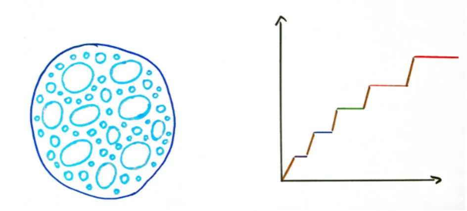
Second order phase transitions exhibit scale invariance at the critical points where the transition occurs. Which can often be lifted to a full conformal invariance. Let us mention the example of critical opalescence of water at its boiling point where one can easily see that there would be

(35)

air bubbles of all sizes if the water recipient did not introduce an upper length scale.

Quantum phases are quantum states of matter at zero temperature. They might be described by some microscopic (short-range) Hamiltonian and two such Hamiltonians will belong to the same class if they yield the same macroscopic properties for the system, assumed to be described by some eﬀective quantum ﬁeld theory.

The quantum ﬂuctuations then might depend on some extra parameters of the problem and therefore phase transitions can occur.

Take for example the quantum Hall eﬀect. One can show that its large scale properties are well described by Cern-Simons theory in three dimen-sions which is known to be equivalent to a conformal ﬁeld theory located at the boundary of its physical space, namely a WZW model.

Figure 7: Classical opalescence of water and quantum Hall plateaux.

In this thesis we will not be dealing with what would happen away from equilibrium. Indeed, one might expect conformal symmetry to be broken in that situation, in the presence for example of disorder introducing its own length scale.

Last but not least, let us mention that conformal field theory appears naturally in two ways in string theory, the first one being through the con-formal symmetry of the world-sheet of the string and the second one being through holography and the fact that, similarly as was mentioned in the case of Chern-Simons theory and a WZW model on its boundary, quan-tum gravity theories are expected to be dual to (super-) conformal field theories.

(36)

6. PLAN OF THE THESIS xxiii

6 Plan of the thesis

• In chapter 1, we will recall some mathematical notions that will be need either for technical support or for inspiration in order to some-times achieve their generalization. We will describe some features of the complex geometry first of Riemann surfaces and then of Ka..hler manifolds, recall some definitions and results of the theory of (Kac-Moody) Lie algebras, introduce the notion of Frobenius manifolds and their relation with integrable hierarchies [38], define the Hitchin inte-grable system and its realization of the non-abelian Hodge correspon-dence and we will then end the chapter by some notions of symplectic geometry and the corresponding methods of quantization.

• In chapter 2, we will study the geometry of the Fuchsian (integrable) system, defined as a fibration of the moduli space of Fuchsian differen-tial systems over Riemann surfaces (P →

o

Σ,∇) ∈ MF uchs. To do so, we will ﬁrst construct the non-perturbative spectral curve Σb associated

to a Fuchsian diﬀerential system, the correlators Wn’s satisfying the loop equations and the corresponding homology of cycles Hc₁. It will

be related to deformations δ ∈ T∗_M

F uchs and the underlying special geometry gives a natural conjectural deﬁnition of a non-perturbative τ-function of the theory and we will mention how it should relate to enumerative geometry. What is understood however is the perturba-tive reconstruction of the correlators by the topological recursion in a topological regime. This regime consists in promoting the considered connections to ε-connections ∇ε for some small complex parame-ter ε ∈ C∗ and study the WKB asymptotics of the construction when

ε −→ 0. There, a cameral curve ΣH (Φ(0)₎ emerges, associated to the

Higgs ﬁeld obtained by the limit Φ(0)

= lim

ε→0(ε∇0− ∇ε). The cameral geometry allows to deﬁne the cameral curve topological recursion recon-struction procedure. This gives a natural scheme to compute pertur-batively the generating functions for derivatives of the τ-function of any integrable hierarchy given in Lax form [8]. We apply this scheme to propose a spectral curve for the KdV hierarchy. We end the chap-ter by studying the Topological Type property ensuring that one can

(37)

reconstruct from the usual topological recursion [43] and apply it to the six Painlevé equations and the (p, q) minimal models of Liouville

gravity [10]

• In chapter 3, we turn towards defining the quantum geometry of con-formal field theories with extended algebras of symmetry given by W-algebras. We start by recalling basic definitions and facts about conformal field theories with W-algebra symmetry defined from a chi-ral spin-one current J valued in a dual g∗ of a Lie algebra g of ADE type, including their operator product expansions and Ward identi-ties. We then define the corresponding quantum spectral curve Eb and

show that the usual topological recursion procedure allows to recon-struct the correlation functions with a non-zero number of currents inserted [5]. We then see that what changes is actually that the initial data of the recursion has to be deﬁned from the quantum spectral curve. We then introduce a special geometry ansatz (Seiberg-Witten relations) [35] to propose a scheme to reconstruct perturbatively chiral correlation functions of the theory without insertions of currents, that is M-point correlation functions of Toda lattice quantum ﬁeld theory. • We will then conclude and give a list of possible projects for the future. To conclude this introduction, note that this text is based on the pub-lished paper [10], the pre-prints [9] and [11] and the articles still in prepara-tion [12], [8], [13], [5] and [6] that will hopefully be available soon. [9], [10] and [11] are collected at the end of the text after the bibliography.

(38)

Chapter 1 Mathematical preliminaries

In this section we will present in an informal way some needed mathe-matical material. It is not needed in the sense that we will use all of the following deﬁnitions and results in the developments of this work but rather because it allows one to get much more context around the objects at stake. Almost no proof will be given since everything can be found quite easily in textbooks or in the references that we give here. A few of them will be given nevertheless when they contain useful insights for what will follow.

1 Complex geometry

1.1 Complex curves

Deﬁnition 1.1 Riemann surfaces

A Riemann surfaceΣ is a complex algebraic curve. It is deﬁned as the zero locus of a polynomial expression of two variables P ∈ C[T1, T2], that is

Σ = {(x, y) ∈ C2 | P (x, y) = d e f X i , j Pi , jxiyj = 0} (1-1) immersed in C2.

Proposition 1.2 Space of holomorphic functions

The only holomorphic functions on a Riemann surface are the constants.

(39)

Figure 1.1: A compact Riemann surface.

As a real two-dimensional surface, the topology of the curve is classiﬁed by its genus, an integer g ∈ N such that its ﬁrst homology group is given by

H1(Σ,Z) = Z2g (1-2)

Fundamental theorems

The Riemann-Hurwitz formula helps computing genera of covers. Theorem 1.3 Riemann-Hurwitz

Let Σ −→Σo be a holomorphic map. It realizes a ﬁnite branched cover. Let

d ∈ N∗ be the number of sheets of the cover and g , g ∈ No be the genera of Σo and

Σ respectively. They are related by

2g − 2 = d(2g − 2) + Bo (1-3)

where B is the total index of the branch points, that is the sum of the

number of sheets coalescing at each branch point minus the number of branch points itself.

Deﬁnition 1.4 Divisors on curves

A divisor on the curve Σ is a formal sum of points with multiplicities,

D = n1P1+ · · · + nrPr (1-4) n1, .., nr ∈ Z, P1, .., Pr ∈ Σ. Its degree is the number deg(D) =Pini.

(40)

1. COMPLEX GEOMETRY 3

Figure 1.2: A branched covering.

For any function f on Σ, denote by ( f ) the divisor of its poles and

ze-roes counted with multiplicities (positive for zeze-roes and negative for poles). For any divisor D on Σ, let M0(D) (resp. M1(D)) denote the space of

meromorphic functions f (resp. forms ω) whose poles are at most the ones speciﬁed by D and whose zeroes are at least the ones speciﬁed by D (denoted D ≤ (f ) resp. D ≤ (ω)).

The Riemann-Roch formula helps computing dimensions of spaces of meromorphic functions and forms with given zeroes and poles on a Rie-mann surface in terms of its genus.

Theorem 1.5 Riemann-Roch

Let D be a divisor on a Riemann surface of genus _{g ∈ N}∗.

dimM0_{(−D) = dim M}1_{(D) + deg(D) − g + 1} (1-5)

Example 1.6 Space of holomorphic diﬀerentials

When D = 0, since the only holomorphic functions on Σ are constants, we get

(41)

Theorem 1.7 Riemann’s bilinear identity

Let {Ai}i =1,..2g be an integer basis of H1(Σ,Z) with intersection product deﬁned

as

Ai

\

Aj =

d e f Ii , j (1-6)

for any i , j ∈ {1,..,2g }. Then for any holomorphic one-forms ω,ω0 ∈

H1(Σ,O_Σ), and any generic point z0∈ Σ,

X x∈p(ω) Res z=x µ ω(z)Z z z0 ω0 ¶ − X x∈p(ω0₎ Res z=x µ ω0_(z) Z z z0 ω ¶ = 1 2πi 2g X i , j =1 µI Ai ω ¶ (I−1)i , j Ã I Aj ω0 ! (1-7)

where we introduced the notation p(ω) (respectively p(ω0₎) for the set of poles

of ω (respectively ω0_). Newton’s polygon

Deﬁnition 1.8 Newton’s polygon

Newton’s polygon N (P ) associated to the Riemann surface deﬁned by a

polyno-mial P ∈ C[T1, T2]is the convex hull of the set {(i , j ) ∈ Z2|Pi , j 6= 0}.

Figure 1.3: The Newton polygon ofY3X2+ (1 + Y + Y2)¡1 + X + X2_{+ X}3_{¢ + X}4_.

Proposition 1.9 Critical exponents

In a local coordinate z, generic asymptotic directions of the curve immersed in

C2 _{are of the form}

(x ∼∞zp, y ∼∞zq) with p, q ∈ N such that − p

q ∈ Q ∪ {∞} is

(42)

proof:

In a local coordinate in an asymptotic direction of the curve,

½ x∼∞zp

y∼∞zq (1-8)

for some integers p, q ∈ N. In this vicinity, introducing the number mp,q= max

(i , j ) {i p + j q}, (1-9) the leading term of the equation deﬁning the curve reads

X

{(i , j )∈N (P)|i p+j q=mp,q}

Pi , j = 0 (1-10)

The sum can’t reduce to one single term otherwise it would contradict the fact that the corresponding (i , j ) pair belongs to N (P ). Therefore, the sum generically contains two terms thus yielding that the straight line

{(i , j ) ∈ Z2|mp,q = i p + j q} is tangent to N (P ), assertion that contains the wanted result. ■

The genus of a Riemann surface can in most case be computed from its Newton’s polygon but in general, the number of interior points of Newton’s polygon only gives an upper bound to the genus through the following Proposition 1.10 g ≤ #N (P )o

with equality if and only if the singularities of the projectivization of the curve in P2 are non-degenerate and located at (001), (010), (100).

proof:

To prove this inequality we will exhibit a generating family of H1(Σ,O_Σ)

consisting of #

o

N (P ) holomorphic one-forms.

By diﬀerentiating the deﬁning equation along the curve we get the equality

(43)

but generically we can’t have P0

x and P0y vanishing at the same point (which would correspond to a cusp singularity) so that d x

P_y0 = − d d y

P_x0 cannot have a pole at any zero of P0

x (or Py0 either by symmetry) and therefore is a holomorphic form on Σ. This is the starting point and now, for any

(i , j ) ∈ Z2, deﬁne the one-form ωi , j on Σ by ωi , j(x, y) = xiyj_P0d x

y(x,y). By

the previous argument, this diﬀerential form is regular everywhere except maybe at inﬁnity in an asymptotic direction. In such a direction (x ∼∞

zp_{, y ∼}_∞ zq), in a local coordinate _{z ∈ C} and with the notations of the

previous proposition, ωi , j(x, y) ∼ z→∞ z i p+j q zp−1d z P k,ll Pk,lzkp+(l −1)q (1-12) ∼ z→∞ z(i +1)p+j q−1d z zmp,q−qP kp+l q=mp,ql Pk,l (1-13) As seen before, there are generically two distinct terms (k, l ) and (k0, l0)

in the sum of the denominator for which we know that Pk,l + Pk0_,l0 = 0. The

condition for l Pk,l + l0Pk0_,l0 to vanish as well is therefore l = l0 which is

generically equivalent tok = k0 and is thus contradicting the fact that there are two distinct terms. Therefore l Pk,l+ l0Pk0_,l0 6= 0 and

ωi , j(x, y) ∼ z→∞ z (i +1)p+(j +1)q−mp,q−1_{d z} (1-14) ∼ z0_→0 (z 0₎mp,q−(i +1)p−( j +1)q−1_{d z}0 (1-15)

where we have changed the local coordinate to z0 ₌ 1_z. From this last expression we can conclude that ωi , j is holomorphic on Σ if and only if

(i + 1)p + (j + 1)q < mp,q, that is (i + 1, j + 1) ∈ o

N (P ) which concludes the proof. ■

Jacobi variety and theta-functions

Deﬁnition 1.11 Symplectic basis of cycles

A basis {Ai,Bi}i =1,...,g of H1(Σ,Z)such that the intersection product is given for

(44)

1. COMPLEX GEOMETRY 7 Ai \ Aj = 0, Bi \ Bj = 0, and Ai \ Bj = δi , j, (1-16)

is called a symplectic basis or a Torelli marking of Σ. It admits a dual basis ofH1(Σ,O_Σ),{ωi}i =1,...,g normalized on A-cycles, that is for anyi , j ∈ {1,..., g },

I Ai ωj = δi , j, I Bi ωj = d e f τi , j (1-17)

where we introduced the period matrix τ.

Figure 1.4: A symplectic basis of cycles on a torus.

Deﬁnition 1.12 Jacobian of curves

The Jacobian variety of Σ is deﬁned as the g-dimensional torus deﬁned by the

quotient Jac(Σ) = d e f C g_±( Zg + τ · Zg) (1-18)

(45)

We can embed the Riemann surface Σ into its Jacobian Jac(Σ) by

Deﬁnition 1.13 The Abel map

The Abel map at a point z0∈ Σis the embedding deﬁned by

Az0: Σ −→ Jac(Σ) z 7−→ Az0(z) = µZ z z0 ω1, . . . , Z z z0 ωg ¶ (1-19)

Changing the base point z0 amounts to a translation in the Jacobian. Proposition 1.14 Matrix of periods

τ is symmetric and the real matrix I m(τ)is positive deﬁnite.

This allows for the deﬁnition of the following fundamental objects Deﬁnition 1.15 Riemann theta-functions

It is the locally analytic function Θ deﬁned for any u ∈ Cg by

Θ(u;τ) =

d e f

X

m∈Zg

e2πi〈m,u〉+πi〈τm,m〉 (1-20)

where 〈 . , .〉 denotes the canonical scalar product on Cg.

It has simple automorphic properties with respect to the period lattice of the Riemann surface.

Property 1.16 Automorphic of theta-functions

For any u ∈ Cg and l ∈ Zg,

Θ(u + l ;τ) = Θ(u ;τ) (1-21)

Θ(u + τ · l ;τ) = e−πi 〈τl ,l 〉−2πi 〈l ,u〉_{Θ(u ;τ)} _(1-22) Deﬁnition 1.17 Theta divisors

The divisor of the theta-function is the zero locus of the theta-function in the

Jacobian of the Riemann surface Σ. It is a well deﬁned g − 1 dimensional

(46)

Deﬁnition 1.18 Theta characteristics

It is a point χ ∈ Cg _{such that} ₂_{χ = a + τ · b ∈ Z}g

+ τ · Zg. It is said to be odd if

and only if 〈a, b〉is odd. It is otherwise said to be even.

Remark 1.19 A theta characteristic endows a spin structure on Σ, namely a line bundle whose tensor square is the canonical bundle of the curve. Indeed,

χ has vanishing class in Jac(Σ) which is an abelian group isomorphic to the

Picard group of line bundles. This correspondence and the integrality of the characteristic yield the spin structure.

Deﬁnition 1.20 Siegel theta-functions

Let χ = a

2 + τ · b

2 be a odd theta characteristic on Σ. The corresponding Siegel

theta-function is the analytic function Θχ deﬁned for any u ∈ Cg by

Θχ(u;τ) = d e f

X

m∈Zg

e2πi〈m+a2,u+b2〉+πi 〈m+a2,τ·(m+b2)〉 (1-23)

Remark 1.21 Regularity of odd theta-characteristics

The theta-characteristics such that Θχ does not vanish identically are called

regular theta-characteristics. We will assume from now on χ to be regular.

Prime forms and twists

Let z0∈ Σ be a point on the Riemann surface and let φz0 be the map that

sends any point z ∈ Σ to the complex number φz0(z) = Θχ(Az0(z) ;τ). φz0

has exactly g zeroes (including q). Then the holomorphic one-form deﬁned by h = d e f X i =1,...,g µ∂Θ χ ∂ui ¶ |u=0 ωi (1-24)

has exactly g − 1 double zeroes such that ph is a well deﬁned holo-morphic spinor and has exactly g − 1 simple zeroes. Moreover, let χ =

d e f 1

2(n + τ · m) ∈ C

(47)

Deﬁnition 1.22 Fay’s prime form

The prime form Eχis the skew-symmetric (−12, − 1

2)spinor deﬁned on the squared

universal cover Σ ×e Σe by

Eχ(p,e q) =e

d e f

φq(p)

ph(p)h(q) (1-25)

It vanishes linearly on the diagonal and nowhere else. For any choice of coordinates, Eχ(p,e q) =e Θχ(Aq(p);τ) ph(p)h(q) p∼q= p − q pd p d q(1 + O (p − q) 2 ) (1-26)

It can be shown not to depend on the choice of odd spin characteristics χ and we will therefore drop the subscript χ from now on.

Remark 1.23 it is not clear from this local deﬁnition that the prime form is

indeed deﬁned on the universal cover but one can easily check that although E

has no monodromy around A-cycles, it satisﬁes

E (p + Be i,q) = E (e p,e q) ee

−2i π(Aq(p)i+χi)_e−i πτi ,i (1-27)

for any choice of index i ∈ {1,..., g }.

In our following constructions we will need a prime form deﬁned glob-ally on our base curve and not its universal cover. This is the reason to introduce a twist. It consists in compensating the B-cycle monodromies of

E by use of a meromorphic one-form. Deﬁnition 1.24 Twisted prime forms

Let f be a meromorphic one-form on Σ with vanishing A-cycle integrals

I Ai f = 0, and 1 2πi I Bi f = d e f ζi (1-28)

(48)

such that ζ =

d e f (ζ1, . . . ,ζg) ∈ C g

− (Zg + τ · Zg). ζ is called a polarization

and its required property implies that f has singularities. Deﬁne the f-twisted

prime form by Ef(p, q) = d e f E (p,e q)e Θχ(ζ;τ) Θχ(Aq(p);τ) e−Rqpf (1-29) with Rp

q f deﬁned as integrating along the unique homology chain not

inter-secting A nor B-cyles with boundary p − q.

Remark 1.25 The dependence in the odd theta-characteristic χ was reintro-duced in the twisted prime form but in all uses that we will make of prime forms, that is cyclic products of the form Ef(p1, p2) ···Ef(pn, p1) for a given

number n ∈ N∗ of generic points p1, . . . , pn ∈ Σ, the dependence in χ will

disap-pear and the dependence in f will only be through the polarizationζ. Moreover,

the skew-symmetry is broken by the twist.

Proposition 1.26 Globality of the twisted prime form

The twisted prime form Ef is well-deﬁned (−1₂, −1₂) spinor on Σ with essential

singularities at the poles of the meromorphic diﬀerential one-form f of order

≥ 2.

Theorem 1.27 Fay’s identities

Let n ∈ N∗ be a positive integer and consider 2n generic points

p1, q1, . . . , pn, qn ∈ Σ. We have the equality

Θχ¡Aq_i(pi) + ζ ¢ Θχ(ζ) 1≤i , j ≤nDet µ ₁ Ef(pi, qj) ¶ = Q i <jEf(pi, pj)Ef(qi, qj) Q i , jEf(pi, qj) (1-30) Remark 1.28 In the genus g = 0 situation, Fay’s identities reduce to Cauchy’s

identity Det 1≤i , j ≤n µ ₁ pi− qj ¶ = Q i <j(pi− pj)(qi − qj) Q i , j(pi − qj) (1-31)

(49)

We also deﬁne the evaluation of this twisted prime form on a degree 0

divisor on the Riemann surface D = d e f P iαi[pi ] to be Ef(D) = d e f Y i 6=j Ef(pi, pj)−αiαj (1-32) such that when the divisor is taken to be D = p − q, Ef(p − q) coincides with Ef(p, q) for any pair of distinct points (p, q) on the surface.

Klein form, Bergman kernel and third kind diﬀerentials Deﬁnition 1.29 Klein form

The Klein form is deﬁned from a twisted prime form Ef by the formula

B_ζ_{(p, q) =} d e f −

1

Ef(p, q)Ef(q, p) (1-33)

Remark 1.30 The Klein form can be shown as mentioned before to depend only

on the polarization ζ hence the subscript.

Deﬁnition 1.31 Bergman kernel

The fundamental second kind diﬀerential, or Bergman kernel Bm associated

to the symplectic basis of cycles m= {Ai,Bi}1≤i ≤g, is the unique symmetric

bi-diﬀerential such that

I Ai B (z, ·) = 0, I Bi B (z, ·) = ωi, B (p, q) ∼ p∼q d p d q (p − q)2 (1-34)

for any index i ∈ {1,..., g } and generic point z ∈ Σ. It is related to the Klein form by the identity

B (p, q) = Bζ(p, q) − 2πi g X i , j =1 ³ ∂2 i , jl n Θχ(ζ;τ) ´ ωi(p)ωj(q) (1-35) and as a consequence of this identity, it’s right hand side does not de-pend on the choice of polarization ζ.

(50)

Deﬁnition 1.32 Third-kind diﬀerentials

Given two generic points p, q ∈ Σ, deﬁne accordingly two corresponding

third-kind diﬀerentials to be • Klein : ωp−q ζ (x) =_{d e f} Z p q B_ζ_{(x, ·)} (1-36) • Bergman : ωp−q (x) = d e f Z p q B (x, ·) (1-37)

where the integral is once again computed along the only homology chain with vanishing intersection with the symplectic basis m and boundary equal to

p − q. They are both meromorphic one-forms with a simple pole at p (resp. q)

with residue +1 (resp. −1).

1.2 Kähler geometry

Deﬁnition 1.33 Hermitian manifolds

A hermitian manifold is a pair (M , g ) where M is a complex manifold and

g is a hermitian metric, that is a riemannian metric on M as a diﬀerentiable

manifold which is invariant under the action of the complex structure I. It has

a canonical 2-form called the Kähler form of (M , g ) and deﬁned by

Ω(ξ,ζ) = g(I · ξ,ζ) (1-38)

It is also invariant under the action of I.

We will write M instead of (M , g ) for a hermitian manifold, without

specifying the metric g, whenever no confusion is possible.

Property 1.34 Let Ω be the Kähler form of a hermitian manifold M with a

given dimension d i m_C_{M = d ∈ N}∗, then Ω∧d is a nowhere vanishing 2d-form.

Deﬁnition 1.35 Kähler manifolds

(51)

Every Kähler manifold is also a symplectic manifold but the converse is not true and a general symplectic manifold does not have an integrable complex structure compatible with the symplectic form.

Deﬁnition 1.36 Hyperkähler metrics

A hyperkähler metric on a 4d-dimensional manifold M is a riemannian metric

g which is kählerian with respect to three complex structures I , J and K that

satisfy the algebraic identities of the quaternions,

I2_{= J}2_{= K}2 _{= −1,} (1-39)

I J = −J I = K , (1-40)

J K = −K J = I , (1-41)

K I = −I K = J. (1-42)

Corresponding to each complex structure is a Kähler form,

ω1(ξ,ζ) = g(I · ξ,ζ), ω2(ξ,ζ) = g(J · ξ,ζ), ω3(ξ,ζ) = g(K · ξ,ζ), (1-43)

and furthermore this set of symplectic (Kähler) forms determines the metric uniquely.

Figure 1.6: A hyperkähler manifold has a CP1_{of complex structures.}