Publisher’s version / Version de l'éditeur:
Journal of the Acoustical Society of America, 54, 5, pp. 1131-1137, 1973-09-01
READ THESE TERMS AND CONDITIONS CAREFULLY BEFORE USING THIS WEBSITE. https://nrc-publications.canada.ca/eng/copyright
Vous avez des questions? Nous pouvons vous aider. Pour communiquer directement avec un auteur, consultez la première page de la revue dans laquelle son article a été publié afin de trouver ses coordonnées. Si vous n’arrivez pas à les repérer, communiquez avec nous à PublicationsArchive-ArchivesPublications@nrc-cnrc.gc.ca.
Questions? Contact the NRC Publications Archive team at
PublicationsArchive-ArchivesPublications@nrc-cnrc.gc.ca. If you wish to email the authors directly, please see the first page of the publication for their contact information.
NRC Publications Archive
Archives des publications du CNRC
This publication could be one of several versions: author’s original, accepted manuscript or the publisher’s version. / La version de cette publication peut être l’une des suivantes : la version prépublication de l’auteur, la version acceptée du manuscrit ou la version de l’éditeur.
Access and use of this website and the material on it are subject to the Terms and Conditions set forth at
Calculation of the radiated field from the vibrational velocity of a wall in
a reverberant field
Donato, R. J.
https://publications-cnrc.canada.ca/fra/droits
L’accès à ce site Web et l’utilisation de son contenu sont assujettis aux conditions présentées dans le site LISEZ CES CONDITIONS ATTENTIVEMENT AVANT D’UTILISER CE SITE WEB.
NRC Publications Record / Notice d'Archives des publications de CNRC:
https://nrc-publications.canada.ca/eng/view/object/?id=98bd537a-b062-42d4-b4a6-c3e21a374cf2 https://publications-cnrc.canada.ca/fra/voir/objet/?id=98bd537a-b062-42d4-b4a6-c3e21a374cf2LE CALCUL DU CHAMP DE RAYONNEMENT
MOYEN DE LA VITESSE DE VIBRATION DUN MUR
DANS UN CHAMP DE REVERBERATION
SOMMAIRE
L'auteur mesure 1'Cnergie de rayonnement d'un mur qui vibre et la compare avec la valeur obtenue d'une connaissance de la corrClation de la vitesse de vibration
Reprirbted f r o ~ n : The Journal of the Acoustical Society of America
Calculation
sf
the radiated field from the vibrational velocity of a wall
in
a reverberant field
R.
J.
DonatoNational Research Council of Canada Division of Building Research, Montreal Road Ottawa Ontario
(Received 10 January 1973)
The radiated energy from a vibrating wall is measured and compared to the value calculated from a knowledge of the correlation of the vibrational velocity over the wall surface. Detailed measurements were made on a single wall, but it is shown that the case of a double wall may be predicted with fair accuracy.
Subject Classification: 2.9.
INTRODUCTION
Sound-transmission loss measurements are commonly made on walls (or floors) between two rooms. With a sound source in one room, the reduction in average sound-pressure level between rooms is measured; this information, together with the area of the separating partition and the absorption in the receiving room, permits calculation of the transmission loss. There are circumstances, however, in which this conventional method does not work well. For example, if there were too much extraneous noise in the receiving room the sound transmitted through the wall could not be mea- sured; then it would be more convenient to measure the wall-surface velocity and calculate the transmitted pressure. I n other situations there may be more than one component to be tested and vibration transducers fixed to each component would enable the effects of each to be computed. A similar case is where flanking problems are present and their effect must be identified and allowed for.
Various attempts have been made in the past to calculate the radiated pressure field from velocity measurements on a vibrating wall. Utley and Mul- hollandl made assumptions about the range of coherence of the sound incident on the panel and calculated expressions for the radiation impedance. Their choice of parameter was arbitrary, and they point out that one really needs to know the correlation function of the velocity over the wall. They still, however, found a large discrepancy between the measured velocity and that calculated from the mass law. This is somewhat surprising, inasmuch as the mass law predicts the transmission loss a t the low frequencies much better than their 25-dB discrepancy would lead one to expect. Price and
Cracker:
using the statistical energy ap- proach: once again obtained discrepancies a t the lower frequencies. Even allowing for the correction made in the analysis, the difference is around7
dB a t the lowest frequency of 100 Hz. I n all cases the velocity a t low frequencies is higher than one would expect. Again themeasurements of transmission loss are higher than their u
theory predicts a t the low frequencies. Better results were obtained when they used a measured value of radiation resistance rather than that calculated by Maidanik.4
I t is important to consider how this radiation resist- ance was measured. Price and Crocker use a shaker attached to the wall and this is effectively a point source. Thus the Hankel k transform of the input force is given by
m
F(k) = 2 1 1 f(r)J~(kr)rdr (1) and if the range of action of f (7) is very small so that
f (r)2nrdr= FQ, then
F(k)=Fo. (2)
Thus the wall is actuated by a wide-band k signal. When, on the other hand, the signal comes from a reverberant field, where the correlation function is (sink,r)/k,r (where k,=w/c, and c the velocity of sound in air), then the Hankel transform is G(k), where
This equals zero for k> k,, and
2n(k,)-l(ka2-k2)-f, for k l k , . (4) Here the k spectrum is restricted to values less than or equal to k,. Thus, it seems reasonable to suppose that the velocity obtained using a shaker will be relatively larger than that obtained using a reverberant incident sound field.
Although it is true that the above argument holds only for an infinite wall, the effect of limiting the dimensions will be to multiply the k spectrum by a The Journal of the Acoustical Society o f America 1131
k domain so that
,
we finally obtain for the correlation functionP,,(~)[H(w)]~e~~~dw,
(7)
contribution' The nonresonant effect be-where P,,, is the cross correlation a t w between the two
Omes important for a large because the
wide-band signals, and H(w) is the transfer function of Maidanik radiation resistance is proportional to the
the filter whose impulse response is h(r). perimeter rather than the area.
As we are interested in the spatial cross-correlation, The approach adopted in this paper is a quasiclassical
we put r = in the above and obtain one in that we assume the modes to be plentiful enough
for the classical equations to be used (probably violated a t the lower frequencies unless the bandwidth is large), but some allowance must be made for the finite size of the wall. Thus the incident sound field is modified by
the aperture in such a way that a convolution must be If R,, is an even function in 7, P,, is an e made between the incident k spectrum and the k w and
spectrum of the wall aperture. This has the effect of
broadening the spectrum to beyond k , and introducing a a P Z U ( ~ ) [ H ( ~ ) ] 2 d ~ discrepancy between the pressure calculated from the
velocity and that actually measured. If R,, is not even in T, we simply have to t
component to obtain an equivalent expressio
I. T D O R Y OF METHOD USED TO
OBTAIN SPATIAL CORRELATION 11. METHODS OF DETERMINING SPATIAL
One way to measure the spatial correlation between CROSS CORRELATION
pick-ups attached to the vibrating wall in a narrow band Three methods were used to determine the spatial of frequencies would be to pass the two signals through cross correlation of the vibration of the wall as a the filters first and then correlate. If we remember, function of frequency.
however, that it is spatial correlation a t zero time
interval that we wish to measure, a more elegant A. Method 1 : Band-by-Band Correlation
procedure would be to cross-correlate the wideband signals first, convert the time-domain correlation signal into its Fourier components, and then operate on the resulting spectra with a suitable narrow-band filter.
If we consider the broad-band signals from the pick- ups to be represented by x(t), y ( ~ ) , the impulse response of the two filters by h(t) and the desired signals to be correlated by el(t) and e2(t) we may write from the convolution theorem :
The cross correlation of el(t), e2(t) may be now written as
If we carry out the normal Fourier conversions on this
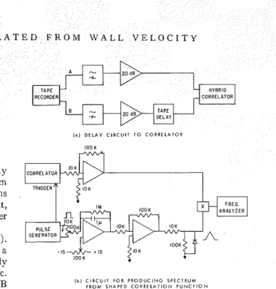
The arrangement is illustrated in Fig. 1. The signals from the two channels to be correlated were ~ a s s e d through two identical filters, then through two inte- grators to convert the signals from accelerations to velocities. (This step is optional; we are measuring spatial correlations in the true sense of the word, where the cross correlation is normalized by dividing by the square roots of the autocorrelations of the two chan- nels.) The two signals then enter an analog multiplier whose output is averaged with a long time constant and displayed.
B. Method 2 : Analogue Operation on
Wide-Band Signal
Both this method and the next method to be de- scribed use a hybrid correlation technique. The previous theoretical derivation has shown that we may first correlate in time using wideband signals and derive the zero time spatial correlation by subsequent Fourier analysis of the correlator output. The analog method described in this section is less attractive than the digital method of the next section, owing to the limita- tions of the correlator. The correlator has available a t its output terminal the correlation of the two inputs, but the output is only one-sided in time. T o do a Fourier analysis of the correlator output in time we need a 1132 Volume 54 Number 5 1973
( o ) D E L A Y C I R C U I T T O C O R R E L A T O R FIG. 1. Narrow-band analog circuit. I O O K
( b ) C I R C U I T F O R P R O D U C I N G S P E C T R U M F R O M S H A P E D C O R R E L A T I O N F U N C T I O N
gave a time delay between the two channels of 0.15 sec.
Some prewhitening was included in each channel and obtained the spatial correlation a t a particular fre- 20 dB of amplification applied. quency. I n order to determine the sound power radiated The remainder of the analyzing process is shown in from the wall, we now need to transform from the space Fig. 2(b). The correlator output is multiplied by a domain to the wavenumber domain. As we are dealing window shaping function in an analogue multiplier. with a two-dimensional distribution of correlation This allows either 0.1 sec of the correlator output to be function, the normalized Hankel transform H ( k ) will be provided to a superheterodyne spectrum analyzer or a used where
triangularly modulated version (Bartlett Window). The correlator output is made repetitive with a period of 63 msec and the frequency analyzer bandwidth taken to be and
1 Hz. The output from the analyzer was frequency m
swept in time and a smoothed version applied to a level R,,(r) =
/
X(k) Jo(kr)kdk. (11)recorder operating in the dc mode. 0
Three methods were used which will now be described. C. Method 3 : Hybrid Operation on
Wide-Band Signal Metlzotf A . The first method used the direct computa-
In essentials, this method is similar to that described tion of the FIanltel transform, using a spatial window of in the previous section, except that here the correlation either unifornl weighting to a masimum correlation output is obtained in digital form and recorded on a distance of 48 in. or a FIanning one, also to m a ~ i m u m printer. The subsequent windows are applied by digital distance. Although the method has the advantage of filtering in a computer. The basic arrangement is shown being the most direct, it does tend to weight the more in Fig, 3. When possible, the windows were taken to be distant points where the experimental accuracy in either a 1/3 or 1/1 octave. determining the correlation function is the least.
Most of the data were obtained using Method 3,
which was found to be more flexible than the other two. MeLh~d I n this method we fit a curve to the exPeri-
some
of the data froln tile other two methods mentally derived correlation function, which we knowhowever, used in the analysis.
D I G I T A L
111. DETERMINATION OF HANKEL TRANSFORM C O R R E L A T O R VOLT - P R I N T E R
OF SPATIAL CORRELATION FUNCTION M E T E R
From the Fourier transforms P,,(w) of the correlation PULSE
function in time of two spaced detectors we have FIG. 3. Wide-band digital system.
R . J . D O N A T O
increased. The frequency in the 400-Hz region. The transducers were his ceramic accelerometers mounted on short lengths of rod a t screwed into the wall. The accelerometers were spaced d about the center of the wall, parallel to the length (10 f t ) n and height (8 ft). Spacings between adjacent trans-
e ducers varied from 2 to 16 in. in a geometric progression. transfer function of the wall. The value of ko was chosen Five transducers were used so that we were able to by computer to correspond to the first zero of the make correlation measurements at 2, 4, 6, 8, 12, 16, 24, correlation function, and a subsequently determined by 32,48, and 64 in. The wall formed the partition between a least squares fit. two reverberant enclosures. The transmitting room was actuated from loudspeakers by a noise signal in the band Method C. This last method once again assumes that the 70 to 7000 Hz. The signals were processed in a wideband correlation function is of the form e-arsinkor/kor but form and filtered in 1/3 or 1/1 octaves. For the wide- employs a slightly more devious method to determine a band case we found it advantageous to split the fre- and ko. Basically, the method makes use of the fact that quency band into two regions by using a filter before the the Fourier transform ensures a best fit on a least analog correlator. To analyze signals below 1 kHz we set squares basis to the original function. Proceeding to the upper cut-off just above 1 kHz, and for signals up to calculate the Fourier transform, on the assumption that 4 kHz we set the upper frequency a t 5 kHz. The the correlation function may be expressed as above, correlator measured one-sided correlation and displayed the results for 100 increments of T, the time delay.
F(k) =
1:
e-aIrI (sinkor/kor)e-jkrdr (12) Applying a window equal in width to the total delay gives a bandwidth of (1007)-l. For lower frequencies (less than 1 kHz) 1 0 0 ~ = 10 msec, and for frequencies = 21"
e-m(sinkor/k~) coskrdr (13) greater than 1 kHz, 1 0 0 ~ = 2 msec. Thus for the lower frequencies the sampling frequency was 10 kHz and for [sin(ko+k)r+sin(k~-k)r] the higher frequencies 50 kHz. These are considerably=
1
e-ar (14) higher than the Nyquist sampling frequency and were k or chosen primarily to improve the signal to noise ratio. I n addition to the rectangular bandwidth a Hanning The integrals in Eq. 12 are of the formwindow was applied, increasing the bandwidths by a " sinmxdx factor of 1.7.
I=
1
e-azT- Typical correlation functions, calculated by com- puter, are shown in Fig. 4. The associated k spectra = tarl(m/a). Thus, F(k) = 3 t a n - l r $ ) + t a n - l ( 7 ) ] (15) - - 1 - - 2kol.l - - tan---. - ko 1 - (ko2-k2)/a2Equation 3 may now be used to determine ko and a . If - we assume that a<<ko, then
- F(k0)-+F(O) and 1 -
r!]
S-. k ~ k oaka
Also T F(O)--. koIV.
CORRELATION FUNCTIONS AND THEIRASSOCIATED k SPECTRUM
Correlation measurements were made on a light- S E P A R A T I O N I N I N .
weight concrete wall (24 lb/ft2) having a coincidence FIG. 4. Correlation coefficients a t octave spacing. 1134 Volume 54 Number 5 1973
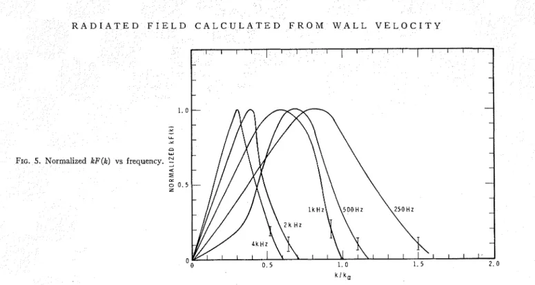
calculated from the Hankel transform are given in Fig. 5. One sees immediately that a t the lower fre- quencies the spectra extend beyond k,=w/c. Thus the finite size of the wall modulates the input correlation function and results in a convolution of the input k spectrum with that of the wall.
Simple reasoning may be applied to explain the form of the spatial correlation functions and their variation with frequency. Figure 6 shows the distance at which the &st zero of the spatial correlation function occurs. We shall simplify the situation by assuming the wall area to be infinite. If the power k spectrum of the incident excitation is F(k) and the impedance of the wall z(k), then the corresponding k spectrum of the velocity is given by
and the corresponding spatial correlation of the velocity will be proportional to R,(r), where
with
E the Young's modulus of the plate, a Poisson's ratio, h the thickness, p, the density, and m=p,h. The char- acteristic impedance of the air surrounding the wall is PC.
As we are considering an infinite wall, the upper limit in the integral of Eq. 21 is k,. For low frequencies k,<<ko, so that apart from an extra contribution near k= k,, R,(r) should have the same form as the correlation function of the applied sound field, i.e., sink,r/(k,r) for a diffuse field. Zero correlation will occur when k,r= T . For higher frequencies where
k,>>ko, R,(r) will have the form Jo(kor) and will have a zero when kor=2.5, These two points were calculated at f=250 Hz and 4 kHz and are shown to fall on the curve of Fig. 6. For frequencies below 250 Hz the infinite wall situation is grossly violated, the upper
F R E Q U E N C Y . H E R T Z
FIG. 6. Variation of first correlation zero with frequency:
g experimental, o theoretical.
F R E Q U E N C Y . H E R T Z
If the wall had been infinite, the amount of power
FIG. 7. Average values of the ratio (first minimum/first radiated from a circle radius R would have been propor-
maximum).
tional to R , (r)2irrirR2. Thus the modulating function is ( I - Y / R ) ~ . It should be noted that this function is limit in the integral is appreciably larger than k, and the different from that mentioned in a previous papers corresponding value of r for zero correlation is reduced; where the form was 1 - ( r / 2 ~ ) 2 . hi^ latter expression this effect may be seen from the curve of Fig. 6. was obtained as an extrapolation from the linear
One other feature of the correlation curve we can look problem, but it is now thought to be less accurate th a t is the amplitude of the first trough. On the above the new expression. The effect on the results of t reasoning, we would expect these to be 0.21 a t low prev~ous paper will be discussed later.
frequencies and 0.40 at higher frequencies. The results
one
further correction ismade for the variation of the are not so accurate as those using the zero values owing rms value of velocity over the wall face.we
find by to scatter in the results a t the larger kr values. The experiment that we may express the velocity astrend is clear, however, and may be seen in the curve of Fig.
7.
V 2 ( r ) = V 2 ( 0 )
V. EFFECT OF FINITE WALL ( l + a ~ / R ) ~
When we come to calculate the power W radiated per Thus the correction to apply is unit area from the wall, we take the Hankel transform
of the velocity correlation function, i.e., [v(k)]" multi-
jR
2 i r r V 2 ( 0 ) d r / /ply by [l-k2/ka2]-4 and integrate from 0 to k,, i.e., 2irrV2(0)dr.
o ( l + a ~ / R ) ~
"
[v(k>12-2irkdkpc. (23) Both a and n may be determined and thence the proper [I
-
k2/km2]: correction.This expression contains v(k), the normalized ve-
VI.
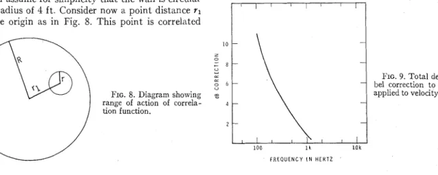
COMPARISON OF MEASURED AND locity, so that we must multiply by the rms velocity CALCULATED PRESSURES squared vo2 tomeasure the true power per unit area. Theexpression holds only for an infinite area wall. To allow Figure 9 shows the total correction to be applied to for the fact that the wall is finite, we must apply a the wall velocity to be applied to the term p c ( ~ o ) 2 ~ for modulating function so that the higher separations the power radiated from the wall. S is the area and Vo
contribute a smaller amount to the correlation function. the rms value of the velocity a t the center. The corn- We shall assume for simplicity that the wall is circular
with a radius of 4 ft. Consider now a point distance r ~ from the origin as in Fig. 8. This point is correlated
! , I 1 1
/ / I
Z 8
FIG. 9. Total deci-
o 6 be1 correction to be
FIG. 8. Diagram showing g applied to velocity.
range of action of correla- 4
tion function.
100 1 k 10 k F R E Q U E N C Y I N H E R T Z
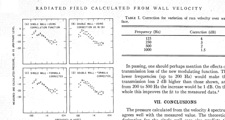
CORRECTEO 3 -10 o o Qed. D z -20 d i . . . o , 0 . - 3 0 100 I K I 0 K CORRECTEO FREQUENCY IN HERTZ
FIG. 10. Comparison of measured and calculated receiving room
pressures: 0 calculated, o measured. (a) Single wall-using
correlation function. (b) Double wall-using same correction as in (a). (c) Single wall-formula corrected. (d) Double wall-formula corrected.
parison of the measured receiving room pressure and the pressure calculated from the wall velocity is given in Fig. 10(a). The biggest discrepancy occurs a t the higher frequencies and is most probably a resonance in the transducer mounting system. Figure 10(b) shows similar results for a double wall (9 lb/ft2). The correla- tion function was not measured for this wall and we applied the single wall correction. Clearly the results are not so good. This is not surprising, because the velocity k spectrum will be different in the two cases. Once again we found a discrepancy at the high frequencies. The velocity results were corrected in this case by comparing the accelerometer output with those from semiconductor strain gauges and a correction applied.
These results may be compared with those calculated using the method given in Ref. 5. There, considering the transmission through a double wall, we convolved the incident k spectra with the k spectrum of the modulating function of the correlation. Making allowances for the fact that we are now using ( ~ - - Y / R ) ~ rather than [I- ( Y / ~ R ) ~ ] , we obtain the results of Fig. 10(d). I t will be seen that thev fit somewhat better. The pro- cedure is repeated for the single wall, only now the analysis is slightly more accurate in that we will apply the modulating function to the velocity itself. For low frequencies, we assume V(k) to be constant from k= 0 to k= k,, and we obtain the results of Fig. 10(c). The fit is almost as good as that using the measured correlation functions.
In passing, one should perhaps mention the effects on transmission loss of the new modulating function. The lower frequencies (up to 200 Hz) would make the transmission loss 2 dB higher than those shown, and from 200 to 500 Hz the increase would be 1 dB. On the whole this improves the fit to the measured data.5
VII. CONCLUSIONS
The pressure calculated from the velocity k spectrum agrees well with the measured value. The theoretical derivation for the single wall case also predicts the pressure reasonably well. For the double wall the theoretical prediction is not so good. When applying the theoretical correction, we have taken the aperture modulating function to apply to the velocity of the surface of the wall rather than to the incident sound field. Thus in the double wall case we apply the modu- lating function to (1-k2/ka2)-4 which, although of the correct general shape, is perhaps not really peaked enough. By applying a more highly peaked function we would obtain the larger discrepancies between velocity . and pressure that we need.
One interesting feature in the single wall case was that although the velocity k spectra showed some variation for different windows (and, hence, bandwidth) the correction to the radiated field showed remarkable consistency.
ACKNOWLEDGMENT
This paper is a contribution from the Division of Building Research, National Research Council of Canada, and i s published with the approval of the Director of the Division.
'W. A. Utley and K. S. Mulholland, "Measurement of Transmission Loss Using Vibration Transducers," J. Sound Vib. 6 (3), 4 1 9 4 2 3 (1967).
'A. J. Price and M. J. Crocker, "Sound Transmission Using Statistical Energy Analysis," J. Sound Vib. 9, 4 6 9 4 8 6 (1969).
'R. H. Lyon and G. Maidanik, "Power Flow between Linearly Coupled Oscillators," J. Acoust. Soc. Am. 34, 6 2 3 6 3 9 (1962).
4G. Maidanik, "Response of Ribbed Panels to Reverberant Acoustic Fields," J. Acoust. Soc. Am. 34, 809-826 (1962). 'R. J. Donato, "Sound Transmission Through a Double-Leaf
Wall," J. Acoust. Soc. Am. 51, 807-815 (1972).