HAL Id: hal-01433518
https://hal.archives-ouvertes.fr/hal-01433518
Submitted on 3 Apr 2017
HAL is a multi-disciplinary open access
archive for the deposit and dissemination of
sci-entific research documents, whether they are
pub-lished or not. The documents may come from
teaching and research institutions in France or
abroad, or from public or private research centers.
L’archive ouverte pluridisciplinaire HAL, est
destinée au dépôt et à la diffusion de documents
scientifiques de niveau recherche, publiés ou non,
émanant des établissements d’enseignement et de
recherche français ou étrangers, des laboratoires
publics ou privés.
LIUM SPKDIARIZATION: AN OPEN SOURCE
TOOLKIT FOR DIARIZATION
Sylvain Meignier, Teva Merlin
To cite this version:
Sylvain Meignier, Teva Merlin. LIUM SPKDIARIZATION: AN OPEN SOURCE TOOLKIT FOR
DIARIZATION. CMU SPUD Workshop, 2010, Dallas, United States. �hal-01433518�
LIUM SPKDIARIZATION:
AN OPEN SOURCE TOOLKIT FOR DIARIZATION
Sylvain Meignier, Teva Merlin
LIUM – Universit´e du Maine, France
ABSTRACT
This paper presents an open-source diarization toolkit which is mostly dedicated to speaker and developed by the LIUM. This toolkit includes hierarchical agglomerative clustering methods using well-known measures such as BIC and CLR. Two applications for which the toolkit has been used are presented: one is for broad-cast news using the ESTER 2 data and the other is for telephone conversations using the MEDIA corpus.
Index Terms— Speaker, Diarization, Toolkit 1. INTRODUCTION
In the NIST terminology, the process of diarization consists in anno-tating temporal regions of audio recordings with labels. The labels represent names of speakers, or their gender, the channel type (nar-row bandwidth vs. wide bandwidth), the background environment (quite, noise, music...), or other characteristics present in the signal. In the case of speaker diarization, the ”who spoke when” annota-tion is performed without any prior informaannota-tion: neither the number of speakers, nor the identities of the speakers, nor samples of their voices are needed. The labels representing the speakers are automat-ically generated without matching the real identities of the speakers. A common approach for this task consists in detecting homogeneous audio segments, which each contain the voice of only one speaker. Then the generated segments are grouped into clusters, one speaker at a time.
The main recent methods are based on hierarchical clustering. The methods differ in choices of merging distance, of the stopping criterion and of the cluster model type (either mono-Gaussian mod-els or Gaussian Mixture Modmod-els (GMMs)). The architecture of the system is partly guided by the nature of the documents it will be used on. According the results obtained in evaluation campaigns, systems can obtain very good results over broadcast news recordings by us-ing BIC clusterus-ing followed by a CLR-like clusterus-ing [1, 2]. Systems based on HMM-BIC [3] or T-test distance [4] perform better than BIC clustering over meeting recordings. Whereas E-HMM shows better performance over telephone conversations [5].
Several toolkits distributed under open-source licenses are avail-able on the web. One of the oldest is the CMU Segmentation toolkit which was released in 1997 [6] and was developed for the NIST broadcast news evaluation campaign. AudioSeg, under the GPL li-cense, is a toolkit developed by IRISA during the ESTER 1 cam-paign in 2005. It includes an audio activity detector, BIC or KL2 segmenting and clustering tools and a Viterbi decoder. Mistral Seg, under the GPL license, is dedicated to speaker diarization and relies
This research was supported by the ANR (French National Research Agency) under contract numbers ANR-06-MDCA-006 and ANR-08-CORD-026-01.
on the ALIZ ´E speaker recognition library. It was the starting point for the development of LIUM SpkDiarization.
The LIUM SpkDiarization toolkit can be used in various ways, to target diverse applications.
In its default configuration, it is oriented towards speaker di-arization of broadcast news. The resulting didi-arization is well suited for speech recognition: each segment is from a single speaker over a single channel with a length shorter than 20 seconds. This system is described in section 2.1. The LIUM transcription system based on Sphinx, used during the ESTER 2 campaign, was described in [2].
The toolkit provides elementary tools, such as segment and clus-ter generators, decoder and model trainers. Fitting those elementary tools together is an easy way of developing a specific diarization system. Section 2.2 shows how to build a diarization system for telephone conversations.
Technical information on how to use the toolkit is given in sec-tion 3. Moreover, it is easy to extend the toolkit by adding algo-rithms. Section 4 describes the main classes and algorithms avail-able.
2. APPLICATIONS 2.1. Broadcast news diarization
The proposed diarization system was inspired by the system [1] which won the RT’04 fall evaluation and the ESTER 1 evaluation. It was developed during the ESTER 2 evaluation campaign for the transcription and diarization tasks, with the goal of minimizing both word error rate and speaker error rate.
Automatic transcription requires accurate segment boundaries. Although non-speech segments must be rejected in order to min-imize insertion of words and to save computation time, segment boundaries have to be set within non-informative zones such as filler words. Indeed, having a word cut by a boundary disturbs the lan-guage model and increases the word error rate.
Speaker diarization needs to produce homogeneous speech seg-ments; however, purity and coverage of the speaker clusters are the main objectives here. Errors such as having two distinct clusters (i.e., detected speakers) corresponding to the same real speaker, or con-versely, merging segments of two real speakers into only one clus-ter, get heavier penalty in the NIST time-based evaluation metric than misplaced boundaries [7].
The system is composed of acoustic BIC segmentation followed with BIC hierarchical clustering. Viterbi decoding is performed to adjust the segment boundaries. Music and jingle regions are re-moved using GMMs, and long segments are cut to be shorter than 20 seconds. A hierarchical clustering using GMMs for speaker models is computed over the clusters generated by the Viterbi decoding.
2.1.1. System description
The Sphinx 4 tools are used for the computation of features from the signal. For the first three steps described below, the features are composed of 13 MFCCs with coefficient C0as energy, and are not
normalized (no CMS or warping). Different sets of features are used for further steps, similarly computed using the Sphinx tools.
Before segmenting the signal into homogeneous regions, a safety check is performed over the features. They are checked to ensure that there is no sequence of several identical features (usually resulting from a problem during the recording of the sound), for such sequences would disturb the segmentation process.
Segmentation based on BIC
A pass of distance-based segmentation detects the instantaneous change points corresponding to segment boundaries. The proposed algorithm is based on the one described in [6]. It detects the change points through a generalized likelihood ratio (GLR), computed us-ing Gaussians with full covariance matrices. The Gaussians are estimated over a five-second window sliding along the whole signal. A change point, i.e. a segment boundary, is present in the middle of the window when the GLR reaches a local maximum.
A second pass over the signal fuses consecutive segments of the same speaker from the start to the end of the record. The mea-sure employs ∆BIC, using full covariance Gaussians, as defined in equation 1 below.
The well known measures for segmentation task are the KL2 [6], the Gaussian divergence [1] and ∆BIC [8]. All of them are imple-mented in this toolkit.
BIC Clustering
The algorithm is based upon a hierarchical agglomerative clustering. The initial set of clusters is composed of one segment per cluster. Each cluster is modeled by a Gaussian with a full covariance matrix. ∆BIC measure is employed to select the candidate clusters to group as well as to stop the merging process. The two closest clusters i and j are merged at each iteration until ∆BICi,j> 0.
∆BIC is defined in equation 1. Let |Σi|, |Σj| and |Σ| be the
determinants of gaussians associated to the clusters i, j and i + j. λ is a parameter to set up. The penalty factor P (eq. 2) depends on d, the dimension of the features, as well as on niand nj, refering to
the total length of cluster i and cluster j respectively.
∆BICi,j= ni+ nj 2 log |Σ|− ni 2 log |Σi|− nj 2 log |Σj|−λP (1) P = 1 2 „ d +d(d + 1) 2 « + log(ni+ nj) (2)
This penalty factor only takes the length of the two candidate clusters into account whereas the standard factor uses the length of the whole data as defined in [8]. Experiments in [1, 9] show that better results are obtained by basing P on the length of the two can-didate clusters only. However, both penalty factors are implemented in the toolkit.
Segmentation based on Viterbi decoding
A Viterbi decoding is performed to generate a new segmentation. A cluster is modeled by a HMM with only one state, represented by a GMM with 8 components (diagonal covariance). The GMM is learned by EM-ML over the segments of the cluster. The log-penalty between two HMMs is fixed experimentally.
The segment boundaries produced by the Viterbi decoding are not perfect: for example, some of them fall within words. In order
to avoid this, the boundaries are adjusted by applying a set of rules defined experimentally. They are moved slightly in order to be lo-cated in low energy regions. Long segments are also cut recursively at their points of lowest energy in order to yield segments shorter than 20 seconds.
Speech detection
In order to remove music and jingle regions, a segmentation into speech / non-speech is obtained using a Viterbi decoding with 8 one-state HMMs. The eight models consist of 2 models of silence (wide and narrow band), 3 models of wide band speech (clean, over noise or over music), 1 model of narrow band speech, 1 model of jingles, and 1 model of music.
Each state is represented by a 64 diagonal GMM trained by EM-ML on ESTER 1 data. The features are 12 MFCCs completed by ∆ coefficients (coefficient C0is removed).
Gender and bandwidth detection
Detection of gender and bandwidth is done using a GMM (with 128 diagonal components) for each of the 4 combinations of gender (male / female) and bandwidth (narrow / wide band). Each cluster is labeled according to the characteristics of the GMM which maxi-mizes likelihood over the features of the cluster.
Each model is learned from about one hour of speech extracted from the ESTER training corpus. The features are composed of 12 MFCCs and ∆ coefficients (C0is removed). The entire features of
the recording are warped using a 3 second sliding window as pro-posed in [10], before the features of each cluster are normalized (centered and reduced).
The diarization resulting from this step fits the needs of auto-matic speech recognition: the segments are shorter than 20 seconds; they contain the voice of only one speaker; and bandwidth and gen-der are known for each segment.
The diarization system developed during the ESTER 2 evalua-tion campaign performs better than the one employed during the first edition of the ESTER campaign: it allowed a gain 0.8 point of word error rate when coupled with the same speech recognition system. GMM-based speaker clustering
In the segmentation and clustering steps above, features were used unnormalized in order to preserve information on the background environment, which helps differentiating between speakers. At this point however, each cluster contains the voice of only one speaker, but several clusters can be related to the same speaker. The contri-bution of the background environment to the cluster models must be removed (through feature normalization), before a hierarchical ag-glomerative clustering is performed over the last diarization in order to obtain a one-to-one relationship between clusters and speakers.
Thanks to the greater length of the speaker clusters resulting from the BIC hierarchical clustering, more robust, complex speaker models can be used for this step. A Universal Background Model (UBM), resulting from the fusion of the four gender- and bandwidth-dependent GMMs used earlier, serves as a base. The means of the UBM are adapted for each cluster to obtain the model for its speaker. At each iteration, the two clusters that maximize a given mea-sure are merged. The default meamea-sures are the Cross Likelihood ratio (CLR) [11] and the Cross Entropy (CE/NCLR) [12, 13]. The GMM-KL2 measure described in [14], equivalent to the Gaussian divergence [1] applied on GMMs, is also available.
The clustering stops when the measure gets higher than a thresh-old set a priori.
2.1.2. Evaluation
The methods were trained and developed according to data from the ESTER/,1 (2003-2005) and ESTER 2 (2007-2008) evaluation cam-paigns. The results of the 2008 campaign are reported in [15]. The data were recorded in French from 7 radio stations, and are divided into 3 corpora: the training corpus corresponding to more than 200 hours, the development corpus corresponding to 20 shows, and the evaluation corpus containing 26 shows.
During the evaluation, the LIUM obtained the best result: 10.80 % of Diarization Error Rate (DER) using the system described in section 2.1, completed by a post-filtering step. The post-filtering consists in removing segments longer than 4 seconds including si-lence, breath, and inspiration, as well as music fillers. Fillers are extracted from the first pass of the speech recognition process [2].
The result was 11.03 % of DER without post-filtering.
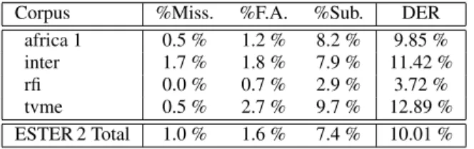
Table 1 shows the current result on the test corpus of ESTER 2: a DER of 10.01 % with no post-filtering. The gain of one point of DER results from improvements in the management of consecutive identical features and of aberrant likelihoods in the Viterbi decoder after the campaign.
Corpus %Miss. %F.A. %Sub. DER
africa 1 0.5 % 1.2 % 8.2 % 9.85 %
inter 1.7 % 1.8 % 7.9 % 11.42 %
rfi 0.0 % 0.7 % 2.9 % 3.72 %
tvme 0.5 % 2.7 % 9.7 % 12.89 %
ESTER 2 Total 1.0 % 1.6 % 7.4 % 10.01 %
Table 1. DER over the ESTER 2 test corpus
The default set of thresholds was determined using the ESTER 2 development corpus. Thresholds should be adapted for other corpus. Without skills in the field of speaker diarization, this task can be difficult. LIUM SpkDiarization includes an experimental tool that automatically performs the tuning by trying various sets of thresh-olds.
Table 2 shows the DERs obtained over the NIST RT’03 diariza-tion corpus (3 shows of broadcast news in English) before and after tuning the thresholds. A gain of 1.3 point can be observed after tun-ing the thresholds.
Thresholds %Miss. %F.A. %Sub. DER
default 0.2 % 2.5 % 5.0 % 7.65 %
tuned 0.2 % 2.5 % 3.7% 6.36 %
Table 2. DER over the RT’03 test corpus
2.2. Telephone
For the ANR project Port-Media, the LIUM needs to segment and transcribe telephonic conversations drawn from the French corpus MEDIA [16]. This corpus contains telephonic dialogues which were recorded using a Wizard of Oz. Conversations focused on tourist information and hotel booking.
Reusing the toolkit developed for the broadcast news system al-lowed to quickly setup a telephonic diarization system.
2.2.1. System description
12 MFCCs are used, completed by the energy. The MFCCs are not normalized during the speech detection step whereas the cepstral
mean is removed during the speaker detection step. Speech detection
This detection relies on a Viterbi decoding using 3 GMMs corre-sponding to speech, silence, and dial tone. Each GMM is composed of 16 Gaussians with diagonal covariance, and trained via the EM-ML algorithm over 20 recordings (1 hour of data) which were seg-mented automatically and controlled by a human.
Only the speech segments are kept for the next step. Speaker detection
The speaker detection method is based on the E-HMM approach de-scribed in [5].
The conversation model is based on an HMM with 2 states. Each state characterizes a cluster, i.e. speaker, and the transitions model the changes between speakers.
A UBM with 16 diagonal components is trained over 4 hours of speech automatically extracted by the speech detector.
A first speaker model is trained on all the speech data. The di-arization is modeled by a one-state HMM and the speech segments are labeled as speaker S0. A second speaker model is then trained
using the three seconds of speech that maximize the likelihood ratio between model S0and the UBM. A corresponding state, labeled as
S1, is added to the previous HMM.
The two speaker models are adapted according to the current diarization. Then, Viterbi decoding produces a new diarization. The adaptation and decoding steps are performed while the diarization differs between two successive runs.
2.2.2. Evaluation
The development corpus is composed of 9 dialogues (33 minutes) whereas the test corpus is composed of 8 dialogues (23 minutes). In the MEDIA corpus, each part of the conversation was recorded separately. In the evaluated corpus, both parts of the conversation were mixed, and provided as a single channel, 8 kHz signal.
The manual transcriptions of the dialogue are available. The boundaries of the segments were manually checked and corrected to be accurate enough for diarization evaluation.
Table 3 shows the DER obtained through development and eval-uation. The system obtains 2.47 % of DER over the test corpus. This error rate is very low but the task is quite easy: there is a lot of silence among speaker utterances and there is very little speech overlap.
Corpus %Miss. %F.A. %Sub. DER
Dev 2.0 % 1.3 % 1.2 % 4.51 %
Test 1.6 % 0.6 % 0.3 % 2.47 %
Table 3. DER over the MEDIA development and evaluation corpus
3. USING THE LIUM SPKDIARIZATION TOOLKIT LIUM SpkDiarization is written in Java, targeting version 1.6 of the language. It requires a Sun JRE. In order to compile or execute the toolkit, the following 3rd party packages are needed:
• gnu-getopt package to manage command lines with long op-tions.
• lapack package to manage matrices (blas, f2util and lapack). Only the inversion method based on Cholesky decomposition is used, for inversion of full covariance matrices of Gaussians. • Sphinx4 and jsapi packages to compute MFCCs.
3.1. Quick Start
For convenience, those 3rd party packages are included in the precompiled version. This version also includes a UBM, gender models, speech/non-speech models, and MFCC configuration files. The execution of the jar file directly invokes the speaker diarization method dedicated to broadcast news recordings (as described in section 2.1).
3.2. Advanced Use
Most of the tools in the package take a diarization as input and gener-ate another diarization as output. The exceptions are model trainers, which generate a model instead of a diarization.
The main tools allow performing segmentation, silence detec-tion, hierarchical clustering, and Viterbi decoding using GMM mod-els trained with EM or MAP. Another set of tools helps to handle the diarization, models or features files. The typical actions applied to diarizations are: filtering, merging, splitting, printing, or extracting.
Figure 1 shows a sample script for training a UBM. The first call of the java virtual machine initializes the model. The initial model contains one gaussian learned over the training data. Iteratively, the gaussians are split and trained (up to 5 iterations of EM algorithm) until the number of components is reached. The second call trains the GMM using the EM algorithm. After 1 to 20 iterations, the algo-rithm stops if the gain of likelihood between 2 iterations is less than a given threshold.
#!/bin/bash
show="ubm"
# Input segmentation file, %s will be substituted with $show
seg="./%s.seg"
# Where is the mfcc, %s will be substituted with the name of the segment show
fMask="./mfcc/%s.mfcc"
# The MFCC vector description, here it corresponds to 12 MFCC + Energy # spro4=the mfcc was computed by SPro4 tools
# 1:1:0:0:0:0: 1 = present, 0 not present.
# order : static, E, delta, delta E, delta delta delta delta E # 13: total size of a feature vector in the mfcc file # 1:0:0:1 CMS by cluster
fDesc="spro4,1:1:0:0:0:0,13,1:0:0:1"
# The GMM used to initialize EM, %s will be substituted with $show
gmmInit="./%s.init.gmms"
# The output GMM, %s will be substituted with $show
gmm="./%s.gmms"
# Initialize the UBM, ie a GMM with 8 diagonal Gaussian components java -Xmx1024m -cp ./LIUM_SpkDiarization.jar
fr.lium.spkDiarization.programs.MTrainInit --sInputMask=$seg --fInputMask=$fMask --fInputDesc=$fDesc --kind=DIAG --nbComp=8 --emInitMethod=split_all --emCtrl=1,5,0.05 --tOutputMask=$gmmInit $show
# Train the UBM via EM
java -Xmx1024m -cp ./LIUM_SpkDiarization.jar
fr.lium.spkDiarization.programs.MTrainEM --sInputMask=$seg --fInputMask= $fMask --emCtrl=1,20,0.01 --fInputDesc=$fDesc --tInputMask=$gmmInit --tOutputMask=$gmm $show
Fig. 1. Example of script for LIUM SpkDiarization
3.3. Experimental Use
Methods currently under development are stored in a Java package named ”experimental”. Classes of this package may be greatly mod-ified or removed at any time.
In version 3.5 of LIUM SpkDiarization, classes for named iden-tification of speakers are being developed [17]. Classes provide new word transcription containers including named entity annotations, Semantic Classification Tree and methods for named identification
of speakers. However, this development affects other classes, so de-velopers are incited to minimize the connections between experi-mental packages and stable packages.
4. PROGRAMMING WITH THE TOOLKIT 4.1. Containers
There are three main containers: one for show annotation, one for acoustic vectors, and one for models.
Cluster and segment containers
Segment and Cluster objects allow managing a diarization. A seg-ment is an object defined by the name of the recording, the start time in the recording, and the duration. These three values identify a unique region of signal in a set of audio recordings.
A cluster is a container of segments, where segments are sorted first by name of recording, then by start time. A cluster should con-tain segments of the same nature: speakers, genders, background environments, etc.
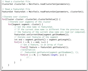
Clusters are stored in an associative container, named Clus-terSet, where the key, corresponding to the name of the cluster, is mapped to the cluster. Therefore, each cluster name should be unique in a ClusterSet. Figure 3 shows the standard way of iterating over clusters and segments. This class design helps data processing when the methods iterate on each segment of each cluster. This access fulfills the majority of the algorithms of hierarchical classifi-cation.
No constraint exists for the relationship of a given acoustic fea-ture to a segment. An acoustic feafea-ture can belong to any one seg-ment or several segseg-ments. No mechanism of checking is provided, and such checking remains the responsibility of the programmer.
ClusterSet clusterMap ... Cluster segmentSet name ... Segment showName startIndex length owner ...
Fig. 2. Incomplete class diagram of ClusterSet, Cluster and Segment Some situations require a temporal sequential access to the acoustic features, while for others random access is preferred, with possible access to cluster membership. Methods are provided to convert a ClusterSet into another container: a ClusterSet can be changed into a set of segments sorted first by record name, then by starting index; or into an array of segments where the index in the array corresponds to the index of an acoustic feature. This last container is available only if the ClusterSet refers to only one recording.
The toolkit uses its own diarization file format. However, di-arizations can be saved to or loaded from files at the Sphinx CTL format that contains the list of utterances to decode.
Acoustic feature container
A FeatureSet stores the acoustic features, which are computed on the fly from the audio recording using Sphinx 4 classes or read from a file containing vectors of parameters. The supported file formats are Sphinx format, SPro4 format, and gzipped-text in which each line corresponds to a vector. The access to acoustic features of a Fea-tureSet is driven by the start index and end index stored in segments.
Common access to the acoustic features is illustrated in figure 3. There are two ways to access to a feature at a given index. The safe method takes two parameters: the name of the recording and the in-dex of the acoustic feature to return. The second way activates the current recording in the FeatureSet before getting the acoustic fea-tures. The second way avoids testing for each feature access whether the current recording is the active one in the FeatureSet.
// Read a clusterSet file.
ClusterSet clusterSet = MainTools.readClusterSet(parameters); // Read a FeatureSet file
FeatureSet featureSet = MainTools.readFeatureSet(parameters, clusterSet); //Iterate over clusters
for(Cluster cluster: clusterSet.clusterSetValue()) { //Iterate over segments of the cluster
for(Segment segment: cluster) { // Set the show name in featureSet.
// If the current show name is different from the previous one, // the features of the current show name are read (or computed). featureSet.setCurrentShow(segment.getShowName());
// Iterate over features of the segment
int end = segment.getStart() + segment.getLength();
for(int i = 0; i < end; i++) {
// Get a feature, ie an array of float
float[] feature = featureSet.getFeature(i); //alternative:
// featureSet.getFeature(segment.getShowName(), i);
for(int j = 0; j < feature.length; j++) { //...
} } } }
Fig. 3. FeatureSet, ClusterSet, Cluster and Segment usage Transformations can be applied before using the acoustic fea-tures. The first and second order derivatives as well as energy and its derivatives can be computed or deleted after reading the raw fea-tures. Feature distribution can be centered and/or reduced, given mean and variance vectors computed over a segment, over a clus-ter, over all the features of the recording, or over a sliding window. Indeed, a FeatureSet gets segments or clusters information from the ClusterSet given as a parameter when the FeatureSet instance is cre-ated. Feature warping is only suitable for sliding windows and can be combined with the previous normalization, before or after.
Section 2.1 shows that systems depend on various acoustic fea-tures. Segmentation and BIC clustering use only static and energy coefficients, speech / non-speech detection needs static and delta, and CLR clustering needed normalized static and delta, etc. Trans-formations reduce the number of feature sets stored on disk. Models
Algorithms need to manage mono-Gaussian models with full or di-agonal covariance or Gaussian Mixture Models (GMMs). Model classes follow the heritage graph shown in figure 4.
Model Scores ... Gaussian ... FullGaussian Accumulator ... DiagGaussian Accumulator ... GMM ...
Fig. 4. Incomplete class diagram of models
The root class ”Model” stores scores: the likelihood of the cur-rent feature, the sum and the mean of likelihoods accumulated by several invocations of the likelihood computation method. Accumu-lators should be initialized before use and reset by setting the accu-mulator to zero. In conjunction with the reset method, those storages permit to easily compute likelihood of a feature, n features, or seg-ments.
Full and diagonal Gaussians implement an inner class to accu-mulate the statistics needed during an EM or MAP training. Those accumulators allow adding or removing weighted acoustic features to/from the accumulator before generating a new model. An illustra-tion can be found in secillustra-tion 4.2.
4.2. Algorithms Training
During the training of a model, the features indexed in the cluster are scanned and EM statistics are stored in the accumulators of the model. After the accumulation, we estimate the model by EM or MAP using the accumulators. The same algorithm is employed for training a mono-Gaussian model and for a GMM. Figure 5 illustrates an iteration of the EM algorithm.
// Initialize the statistic and score accumulators
gmm.initStatisticAccumulator(); gmm.initScoreAccumulator(); for(Segment segment: cluster) {
featureSet.setCurrentShow(segment.getShowName());
// Iterate over features of the segment
for(int i = 0; i < segment.getLength(); i++) {
float[] feature = featureSet.getFeature(segment.getStart()+i);
// Get the likelihood of the feature (1)
double lhGMM = gmm.getAndAccumulateLikelihood(feature); for (int j = 0; j < gmm.getNbOfComponents(); j++) {
// Read the likelihood of component j computed in (1)
double lhGaussian = gmm.getComponent(j).getLikelihood();
// Add weighted feature in the accumulator of the GMM
gmm.getComponent(j).addFeature(feature, lhGaussian / lhGMM); }
} }
// Compute the model according to the statistics
gmm.setModelFromAccululator();
// Reset the statistic and score accumulators
gmm.resetStatisticAccumulator(); gmm.resetScoreAccumulator();
Fig. 5. Training a GMM from a cluster Clustering
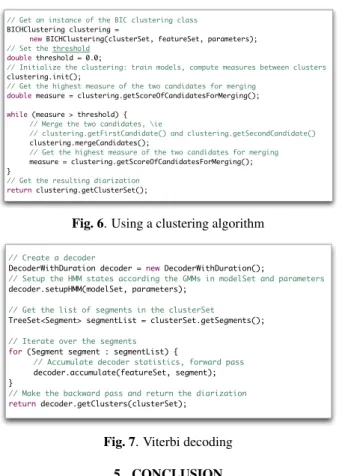
All clustering algorithms follow a bottom-up hierarchical approach (see figure 6). At initialization, the process trains the initial model of each cluster and computes the similarity measures between pairs of clusters. The process continues until the measure gets above a given threshold. According to the measures, at each iteration, the two most similar clusters are merged into a new cluster. During the merging, the model of the new cluster is trained and the similarities between this cluster and others are computed.
Decoding
A basic Viterbi decoder is available and the HMM models are based on the transformation of a set of GMMs. Each GMM is associated with an HMM. By default an HMM contains only one state but the minimum duration can be controlled by duplicating the state to form a string. HMM transition is fixed internally to 0, but the log penalties to switch between two HMMs needs to be set.
Decoding, as presented in figure 7, performs the forward pass in which statistics are accumulated. The best path across the states is defined by a diarization using the GMM name as cluster name. Aligned states are pushed as segments in the corresponding clusters.
// Get an instance of the BIC clustering class
BICHClustering clustering =
new BICHClustering(clusterSet, featureSet, parameters);
// Set the threshold
double threshold = 0.0;
// Initialize the clustering: train models, compute measures between clusters
clustering.init();
// Get the highest measure of the two candidates for merging
double measure = clustering.getScoreOfCandidatesForMerging(); while (measure > threshold) {
// Merge the two candidates, \ie
// clustering.getFirstCandidate() and clustering.getSecondCandidate()
clustering.mergeCandidates();
// Get the highest measure of the two candidates for merging
measure = clustering.getScoreOfCandidatesForMerging(); }
// Get the resulting diarization
return clustering.getClusterSet();
Fig. 6. Using a clustering algorithm // Create a decoder
DecoderWithDuration decoder = new DecoderWithDuration();
// Setup the HMM states according the GMMs in modelSet and parameters decoder.setupHMM(modelSet, parameters);
// Get the list of segments in the clusterSet TreeSet<Segment> segmentList = clusterSet.getSegments(); // Iterate over the segments
for (Segment segment : segmentList) {
// Accumulate decoder statistics, forward pass decoder.accumulate(featureSet, segment); }
// Make the backward pass and return the diarization
return decoder.getClusters(clusterSet); Fig. 7. Viterbi decoding
5. CONCLUSION
This paper presents a diarization toolkit mostly dedicated to speaker. Developed by the LIUM, this toolkit is published under the GPL license. When used for broadcast news diarization, it represents the state of the art in terms of performance. But its components can also be employed for other tasks with only minor work.
An interesting way to improve the toolkit will be implementing some missing methods. For example, methods such as [3, 4] are very useful to develop a system dedicated to meeting diarization.
Efforts should be done to bring the diarization toolkit closer to Sphinx 4. In particular, Sphinx 4 configuration management tools are very flexible and could be an efficient replacement for a number of scripts used with this toolkit. Moreover, the Viterbi decoder and access to acoustic features could adopt the Sphinx interface, thus helping developers to use both toolkits together.
6. ACKNOWLEDGEMENTS
We are grateful to Vincent Jousse and Gael Salaun for their helpful contributions during the development of this toolkit.
7. REFERENCES
[1] C. Barras, X. Zhu, S. Meignier, and J.L. Gauvain, “Multi-stage speaker diarization of broadcast news,” IEEE Transactions on Audio, Speech and Language Processing, vol. 14, no. 5, pp. 1505–1512, 2006.
[2] P. Del´eglise, Y. Est`eve, S. Meignier, and T. Merlin, “Im-provements to the LIUM French ASR system based on CMU Sphinx: what helps to significantly reduce the word error rate?,” in Interspeech 2009, September 2009.
[3] J. M. Pardo, X. Anguera, and C. Wooters, “Speaker diariza-tion for multiple-distant-microphone meetings using several sources of information,” IEEE Transactions on Computers, vol. 56, no. 9, pp. 1212–1224, 2007.
[4] Trung Hieu Nguyen, Eng Siong Chng, and Haizhou Li, “T-test distance and clustering criterion for speaker diarization,” in Interspeech 2008, September 2008.
[5] S. Meignier, D. Moraru, C. Fredouille, J.-F. Bonastre, and L. Besacier, “Step-by-step and integrated approaches in broad-cast news speaker diarization,” Computer Speech and Lan-guage, vol. 20, no. 2-3, pp. 303–330, 2006.
[6] M. Siegler, U. U. Jain, B. Raj, and R.M. Stern, “Automatic segmentation, classification and clustering of broadcast news audio,” in the DARPA Speech Recognition Workshop, Chan-tilly, VA, USA, February 1997.
[7] NIST, “Fall 2004 rich transcription (RT-04F) evaluation plan,” August 2004.
[8] S. Chen and P. Gopalakrishnan, “Speaker, environment and channel change detection and clustering via the bayesian in-formation criterion,” in DARPA Broadcast News Transcription and Understanding Workshop, Landsdowne, VA, USA, Febru-ary 1998.
[9] S. E. Tranter and D. A. Reynolds, “Speaker diarisation for broadcast news,” in Odyssey 2004 Speaker and Language Recognition Workshop, 2004.
[10] J. Pelecanos and S. Sridharan, “Feature Warping for robust speaker verification,” in 2001: a Speaker Odyssey. The Speaker Recognition Workshop (ISCA, Odyssey 2001), Chania, Crete, June 2001, pp. 213–218.
[11] D. A. Reynolds, E. Singer, B. A. Carlson, G. C. O’Leary, J. J. McLaughlin, and M. A. Zissman, “Blind clustering of speech utterances based on speaker and language characteristics,” in Proceedings of International Conference on Spoken Language Processing (ICSLP 98), 1998.
[12] A. Solomonoff, A. Mielke, M. Schmidt, and H. Gish, “Cluster-ing speakers by their voices,” in Proceed“Cluster-ings of International Conference on Acoustics Speech and Signal Processing (IEEE, ICASSP 98), Seattle, Washington, USA, May 1998.
[13] V-B. Le, O. Mella, and D. Fohr, “Speaker diarization using normalized cross-likelihood ratio,” in Interspeech 2007, 2007. [14] M. Ben, M. Betser, F. Bimbot, and G. Gravier, “Speaker diarization using bottom-up clustering based on a parameter-derived distance between GMMs,” in Proceedings of Inter-national Conference on Spoken Language Processing (ISCA, ICSLP 2004), Jeju, Korea, Oct. 2004.
[15] S. Galliano, G. Gravier, and L. Chaubard, “The ESTER 2 evaluation campaign for the rich transcription of French radio broadcasts,” in Interspeech 2009, September 2009.
[16] L. Devillers, H. Bonneau-Maynard, S. Rosset, P. Paroubek, K. Mctait, D. Mostefa, K. Choukri, L. Charnay, C. Bous-quet, N. Vigouroux, F. B´echet, Romary L., J.-Y. Antoine, J. Villaneau, M. Vergnes, and J. Goulian, “The French ME-DIA/EVALDA project: the evaluation of the understanding ca-pability of spoken language dialogue systems,” in LREC, Lan-guage Resources and Evaluation Conference, Lisboa, Portu-gal, May 2004, pp. 2131–2134.
[17] V. Jousse, C. Jacquin, S. Meignier, Y. Est`eve, and B. Daille, “Automatic named identification of speakers using diarization and ASR systems,” in ICASSP, Taipei, China, 2009.