HAL Id: hal-02285149
https://hal.archives-ouvertes.fr/hal-02285149
Submitted on 10 May 2021
HAL is a multi-disciplinary open access
archive for the deposit and dissemination of sci-entific research documents, whether they are pub-lished or not. The documents may come from teaching and research institutions in France or abroad, or from public or private research centers.
L’archive ouverte pluridisciplinaire HAL, est destinée au dépôt et à la diffusion de documents scientifiques de niveau recherche, publiés ou non, émanant des établissements d’enseignement et de recherche français ou étrangers, des laboratoires publics ou privés.
Identification of very large scale structures in the
boundary layer over large roughness elements
Laurent Perret, Franck Kerhervé
To cite this version:
Laurent Perret, Franck Kerhervé. Identification of very large scale structures in the boundary layer over large roughness elements. Experiments in Fluids, Springer Verlag (Germany), 2019, 60 (6), pp.97. �10.1007/s00348-019-2749-7�. �hal-02285149�
Identification of very large scale structures in the boundary layer
over large roughness elements
Laurent Perret1 · Franck Kerhervé2
Abstract
The dynamics of a turbulent boundary layer developing over a cube array is investigated based on stereoscopic PIV meas-urements performed in a boundary layer wind tunnel. The fluctuating streamwise velocity component u′ is analyzed via the
recently introduced Spectral Proper Orthogonal Decomposition method (S-POD). A modification of the definition of the spatial S-POD modes is proposed so that they are orthonormal to each other. This results in spatio-temporal modes which reflect the statistical organization of the most energetic structures both in space and time. It is first demonstrated that the first S-POD modes of u′ correspond to large-scale elongated coherent structures of low or high momentum. The existence of very
large scale structures whose length spans several boundary layer thickness is demonstrated, in agreement with the recent similar findings for flows over smooth wall. These structures are found to be non-negligible contributors to the Reynolds shear stress and the turbulent kinetic energy. Their relationship with the smaller scales of the flow is investigated via the computation of joint third-order statistics and is shown to be of non-linear nature.
* Laurent Perret
1
Centrale Nantes, LHEEA, UMR 6598 CNRS, Nantes, 1 rue de la Noë, BP 92101, 44321 Nantes Cedex 3, France
2 Institut PPRIME, Université de Poitiers - ENSMA, UPR
6609 CNRS, Poitiers, France
1 Introduction
During the past few years, very large scale motions (VLSMs) in turbulent boundary layers over smooth walls have received renewed attention from the research commu-nity. Both numerical and experimental studies have high-lighted their influence on the near-wall turbulence and their contribution to the turbulent kinetic energy and Reynolds shear stress in different types of wall-bounded flows such as pipe flows (Monty et al. 2007), channel flows (del Alamo and Jimenez 2003), laboratory boundary layers (Marusic and
Hutchins 2008) and atmospheric boundary layers (Guala et al. 2011). Common features of the VLSMs found in wall-bounded flows are that they consist of elongated low- and high-speed regions relative to the mean flow populating the logarithmic and outer layers (Hutchins and Marusic 2007). Their streamwise extent scales with boundary layer thick-ness 𝛿 and can reach several times 𝛿 (Guala et al. 2011). They were shown to be animated by a meandering motion in the horizontal plane (Hutchins and Marusic 2007). Mathis et al. (2009) demonstrated that they interact with near-wall tur-bulence through an amplitude modulation mechanism. The
finding of this last characteristic relies on the clear spectral separation between large-scale motions and the near-wall turbulence found in high-Reynolds number flows (Guala et al. 2011; Mathis et al. 2009).
At the same time, attention has been devoted to the structure of boundary layer flows developing over rough walls, at laboratory scales (see Jimenez 2004 for a review) or in atmospheric flows over urban or vegetation cano-pies (Blackman and Perret 2016; Finnigan 2000; Hutchins et al. 2012; Inagaki and Kanda 2010; Perret et al. 2019; Takimoto et al. 2011), demonstrating similarities between flows over smooth and rough walls. In particular, the pres-ence of streaky patterns of low- and high-speed regions, of ejection and sweep motions associated with the hairpin model (Adrian 2007), and the organization of hairpin vor-tices in packets have been evidenced. Recently, Inagaki and Kanda (2010) showed the presence of very large scale elongated low-speed regions with some sub-structures included in these streaks in the atmospheric flow devel-oping over an array of cubes. These structures, identified by filtering the time series in the spanwise direction from a spanwise array of 15 sonic anemometers, share some common features with the VLSMs evidenced in smooth-wall flows. For an atmospheric boundary layer developing over a cubical array arranged in a square pattern, Taki-moto et al. (2011) showed the intermittent presence of large-scale upward motions across the whole wall-normal cross section between two cubes inside the canopy. These were found to be correlated with the presence of low-speed streaks in the boundary layer. A similar organization was observed by Perret and Savory (2013) for a turbulent boundary layer over a street-canyon model. From their particle image velocimetry (PIV) measurements performed over a cube array, Rivet et al. (2012) evidenced the pres-ence of vortex clusters which were intermittently shed off the roughness elements and transported in the boundary layer. They also showed that the dynamics of the associ-ated shear layers developing from the top of the obstacles is correlated with the occurrence of low- and high-speed events in the log region. For the same configuration, using a multi-time delay stochastic estimation technique applied to PIV data in the near-wall region synchronized with hot-wire anemometry (HWA) velocity measurements in the logarithmic layer, Blackman and Perret (2016) succeeded in separating the large-scale contribution of the overlying boundary layer from the flow near the top of the obstacles. Their analysis of the scale-decomposed skewness of the streamwise velocity component demonstrated the non-linear nature of the interaction between these two com-ponents of the flow. They evidenced a multi-scale interac-tion mechanism that resembles the amplitude modulainterac-tion one found by Mathis et al. (2009) in boundary layers over smooth wall, in agreement with the recent findings
obtained by Anderson (2016) from large-eddy simulations of flows over cubical roughness. These findings have been extended by Blackman et al. (2018b) to street canyons of different width, with various upstream roughness con-figuration of urban type. Placidi and Ganapathisubram-ani (2015) recently performed a snapshot-based proper orthogonal decomposition (POD) of PIV measurements obtained in a boundary layer developing over urban-like roughness elements. They explored the spatial character-istics and the behavior of the flow and its dependence on wall morphology. The most energetic modes, containing about 50% of the turbulent kinetic energy, were found to consist of large-scale elongated regions of low and high momentum, whose characteristics proved to be independ-ent of the wall configuration. The results obtained in flows over rough walls suggest that, in spite of the strong dis-turbance of the flow at the wall, VLSMs exist and interact with the canopy flow in a similar manner as in smooth-wall boundary layers. However, sharp edge bluff bodies such as those encountered in urban canopies generate coherent structures of scales much larger than that existing in the near-wall region of a smooth-wall boundary layer (Volino et al. 2011; Perret et al. 2019). Therefore, the clear spectral separation between large-scale motions and the near-wall turbulence found in high-Reynolds number smooth-wall boundary layers may not exist in boundary layer devel-oping of arrays of bluff bodies. As pointed by Takimoto et al. (2011), the knowledge of the connections between the canopy flow and organized structures in the boundary layer is currently still limited.
When aiming at investigating the presence of large-scale structures in a turbulent boundary layer developing over a cubical roughness array and studying their dynamical link with the canopy flow, two challenges then arise. First, the clear spectral separation between the near-wall turbulence and the energetic scales in the logarithmic region found in smooth-wall turbulent flows is not expected to exist any-more. In turbulent boundary layers over rough walls in cases for which the flow is in fully-rough regime, the mean streamwise velocity component reads, when written in its meteorological form (Castro 2007),
where u(z) is the mean streamwise velocity component at height z, u𝜏 the friction velocity, 𝜅 = 0.4 the von Karman
constant, d the displacement height and z0 the roughness
length, equivalent of the streamwise velocity component deficit used in the engineering community. In the fully rough regime, the ratio z0∕h depends only on the roughness
geom-etry and not on the Reynolds number anymore. In urban environment, a typical value of the ratio z0∕h is 0.1 while
(1) u(z) u𝜏 = 1 𝜅log ( z − d z0 ) ,
the ratio 𝛿∕h is comprised between 10 and 20 (Grimmond and Oke 1999; Jimenez 2004). With these values and by extrapolating the log-law up to z = 𝛿 , the ratio between typi-cal temporal stypi-cales in the boundary layer and close to the canopy, T𝛿= 𝛿∕U𝛿 and Th = h∕u𝜏 (where U𝛿 is the integral
velocity scale related to the largest scales, and u𝜏 the friction
velocity), respectively, can be estimated as being close to unity (Perret et al. 2019):
A lack of separation in the spectral domain between the most energetic scales from the boundary layer and those existing near the canopy thus appears to be an intrinsic characteristic of boundary layers developing over urban terrains and can, therefore, be expected in small-scale wind tunnel experi-ments if the flow is correctly scaled (i.e. similarity between model and full scale of 𝛿∕h and the Jensen number z0∕h must
be ensured, Savory et al. 2013). The second challenge arising is an experimental one. Performing reliable measurements of time series of the velocity via multi-component hot-wire anemometry can turn out to be difficult and even impossible due to the high local turbulent intensities and the highly three-dimensional character of the flow close to the canopy top (Perret and Rivet 2018). To circumvent this issue, opti-cal velocimetry methods have been recently employed in flows over urban-like roughness arrays. Herpin et al. (2018) succeeded in performing laser Doppler anemometry (LDA) measurements within the canopy with a sampling rate high enough to allow for the computation of velocity spectra but also cross-spectra between the LDA measurements and the streamwise velocity component measured by HWA in the outer region. Basley et al. (2018) performed stereoscopic PIV in a wall-parallel plane just above the canopy top. The streamwise extent of their PIV data was large enough to allow for the reconstruction of the large-scale motions using Taylor’s hypothesis.
To investigate the interaction between boundary layer and canopy scales, an alternative scale-separating method which can capture the spatial heterogeneities of the flow in the canopy region is proposed. This methods differs from the one now classically used in the literature (Mathis et al.
2009) in that it does not rely on the use of a spectral cutoff filter nor require the use of two-point time-resolved veloc-ity measurements (such as the similar LSE-based methods employed by Blackman and Perret 2016). To circumvent the two above-mentioned issues, the fluctuating streamwise velocity component, measured by low-speed stereoscopic PIV, is analyzed via the use of a modified version of the now well-known POD, the spectral POD (S-POD) recently introduced by Sieber et al. (2016). Benefiting from the band-pass behavior of the S-POD, the goal is to account for the
(2) T𝛿 Th = 𝛿 h u𝜏 U𝛿 = 𝛿 h [ 1 𝜅log ( 𝛿 h h z0 )]−1 .
long-range coherence of the most energetic coherent struc-tures existing in the boundary layer to first extract them and then to allow for the study of their interactions with the near canopy turbulence. The remainder of the paper is organ-ized as follows: the experimental setup, the main character-istics of the flow and the POD procedure are presented in Sect. 2. The results obtained from the proposed POD analy-sis are presented and discussed in Sect. 3. The last section is devoted to the conclusions.
2 Methods
In this section, a description of the experimental appara-tus and procedures and a presentation of the characteris-tics of the generated boundary layer are provided. The obstacle height h has been chosen large enough to ensure both large Reynolds numbers h+= hu𝜏∕𝜈 = 1430 and z+0 = z0u𝜏∕𝜈 = 160 (where 𝜈 is the kinematic velocity) guaranteeing that the flow is in a fully rough regime, and a satisfying spatial resolution of the PIV measurements. The trade-off for obtaining a ratio 𝛿∕h ≃ 20 is the rather limited streamwise extent of the PIV field of view when compared to the typical integral length scales of the boundary layer. It is indeed limited to a fraction of 𝛿 , which constitutes another motivation for the development of a new scale-decomposi-tion method. The obtained scaling ratios 𝛿∕h and z0∕h (see
Table 1) are in the range of those discussed in the introduc-tion, ensuring the investigated flow presents the same char-acteristics as the targeted flow configurations (Cheng et al.
2007; Grimmond and Oke 1999).
In the following, x, y and z denote the streamwise, span-wise and wall-normal directions, respectively (Fig. 1), and u, v, w the streamwise, spanwise and wall-normal velocity components, respectively. Using the Reynolds decomposi-tion, each instantaneous quantity u can be decomposed as u= u + u� where u denotes the ensemble average (equivalent to a time-average) of u and u′ its fluctuating part. The spatial
average over the streamwise extent of the SPIV measurement region of u is denoted ⟨u⟩ . The variance of any quantity u obtained via combined time and spatial is denoted 𝜎2
u.
2.1 Experimental setup
The present experiments were performed in the atmospheric boundary layer wind tunnel of the LHEEA lab, Nantes, France. It has working section dimensions of 24 × 2 × 2 m3
and a freestream velocity range of 3–10 ms−1 . The simulation
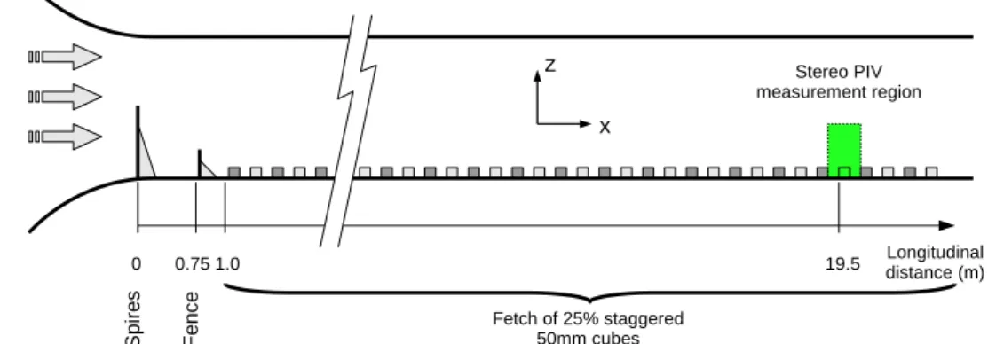
at the scale 1:200 of a suburban-type atmospheric bound-ary layer developing over an idealized canopy model was achieved using three wall-normal, tapered spires of height of 800 mm and width of 134 mm at their base, a 200-mm-high solid fence across the working section located 0.75 m
downstream of the inlet, followed by a 22-m stretch of staggered cube roughness elements with a plan area den-sity of 𝜆p= 25% (Rivet et al. 2012). The cube height was h = 50 mm. The measurements were performed with a freestream velocity, Ue , of 5.77 ms−1 , at a streamwise
loca-tion of 19.5 m after the end of the contracloca-tion. Character-istics of the generated boundary layer are described in the following section. For a complete description and charac-terization of the flow, the reader is referred to the work of Perret et al. (2019).
To fully characterize the boundary layer, single hot-wire measurements were performed along the wall-normal direction throughout the whole boundary layer (Perret et al.
2019). For that purpose, only one location relative to a cube was considered as spatial heterogeneities of the flow induced by the presence of the cubes are confined to the lower region of the flow below z∕h ≃ 2 − 3 . Blackman et al. (2017) and Basley et al. (2018) have indeed shown that second-order statistics and terms in the turbulent kinetic energy budget were uniform in the horizontal plane above that height. A DANTEC 55P11 probe (with a wire length of 1.25 mm cor-responding to l+= lu
𝜏∕𝜈 = 30 to 56 wall units) with a DISA
55M01 electronics was used with an overheat ratio set to 1.8, combined with an eighth-order anti-aliasing linear phase elliptic low-pass filter used before signal digitization. Acqui-sitions were performed during a period of approximately 24,000 𝛿∕Ue using a sampling frequency of 10 kHz. A total
of 39 logarithmically distributed points were sampled. The temperature correction procedure proposed by Hultmark and Smits (2010) was employed and included in a calibration procedure based on King’s law. The probe was calibrated in the freestream flow at the beginning of each half of the profile. Both the form drag and the displacement height d were estimated using the method proposed by Cheng et al. (2007). Distribution of the wall pressure on the back and front faces of a cube obstacle was measured. A cube was manufactured with 36 pressure ports on a wall-normal face to measure the pressure difference between the wall-pres-sure on the cube and the static preswall-pres-sure in the freestream. The cube was rotated to access the pressure distribution on
both the upstream and downstream faces successively. The friction velocity u𝜏 has been obtained from the calculation
of the form drag via the direct integration of the pressure forces onto the instrumented cube. As shown below, the flow being in fully rough regime, the contribution of the viscous forces to the total drag has been neglected (Cheng et al. 2007; Jimenez 2004). Jackson (1981) interpreted the displacement height d as the height at which the drag on the roughness elements is exerted. Therefore, using the same set of mean pressure measurements, the displacement height d was inferred from the calculation of the moment of the pres-sure forces about the base of the cube. The roughness length z0 has been obtained by fitting the measured mean velocity
profile with the logarithmic law of Eq. 1.
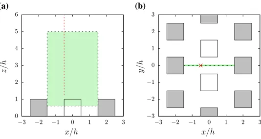
Stereoscopic PIV measurements were conducted in a wall-normal plane aligned with the main flow, in the center of the test section (Fig. 1). Details of the exact location of the measurement plane are shown in Fig. 2. Two 2048 × 2048 pixels2 12-bit camera equipped with Nikon 105 mm AF
Micro objective lenses (at aperture f#= 2.8 ) were employed in a stereoscopic configuration. The Scheimpflug condition was satisfied by rotating the image plane with respect to the lens plane via the use of dedicated remote-controlled mounts. The cameras were mounted outside the test section, on each side of the light sheet in a symmetric configuration, each camera axis forming an angle of 48◦ with the x − z
plane. The final spatial resolution is 1.72 mm (49 wall units) and 2.20 mm (63 wall units) in the streamwise and wall-normal directions, respectively. A Litron 200 mJ Nd–YAG laser, located under the wind tunnel floor, was employed to illuminate the region of interest through a glass window. The laser sheet thickness was estimated as being 3 mm. The time delay between two images for PIV processing was set to dt = 500 μ m, ensuring an average displacement of 13 pixels over the entire region of interest. The flow was seeded with glycol/water droplets (typical size 1 μ m) using a fog gen-erator. Both the synchronization between the laser and the cameras and the calculation of the PIV velocity vector fields were performed using the DANTEC FlowDynamics soft-ware. A set of N = 4000 velocity fields was recorded with
Fig. 1 Wind tunnel layout
(adapted from Blackman and Perret 2016)
a sampling frequency of fs= 5 Hz to enable the computa-tion of the main flow statistics and investigate its large-scale organization. A FFT-based 2D-PIV algorithm with sub-pixel refinement was employed. Iterative cross-correlation analy-sis was performed with an initial window size of 128 × 128 pixels and with 32 × 32 final interrogation windows, using an overlap of 50%. Spurious vectors were detected by an automatic validation procedure whereby the signal to noise ratio of the correlation peak had to exceed a minimum value, and the vector amplitude had to be within a certain range of the local median to be considered as valid. Once spurious vectors had been detected, they were replaced by vectors resulting from a linear interpolation in each direction from the surrounding 3 × 3 set of vectors. A pinhole model was employed to reconstruct the three-component vector fields from the two-component vector fields from each cameras (Soloff et al. 1997; Calluaud and David 2004).
2.2 Boundary layer characteristics
The main characteristics of the investigated boundary layer are summarized in Table 1. As mentioned earlier, the ratio 𝛿∕h and z0∕h are in the range of those expected for the type of targeted urban terrain. Moreover, both the Reynolds num-ber based on the obstacle height h+
and that based on the 99% boundary layer thickness 𝛿+= 𝛿u𝜏∕𝜈 are large enough to ensure that the flow is in the fully rough regime (Jimenez
2004) and that the present boundary layer can be qualified as a high-Reynolds number one. This is confirmed by the value of z+
0 , largely above the critical value of 0.5 reported
by Snyder and Castro (2002). The value of d / h and z0∕h are
in good agreement with those reported in the literature (Cas-tro et al. 2006; Cheng et al. 2007; Grimmond and Oke 1999), confirming the suitability of the present setup for reproduc-ing the aerodynamical characteristics of the targeted flow.
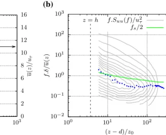
Wall-normal profiles of the mean streamwise velocity obtained from both PIV and hot-wire measurements at a single streamwise location (Fig. 2) are presented in Fig. 3a and show good agreement between each other. Moreover, the profile of the mean streamwise velocity component exhibits a well-developed logarithmic region. An excellent match with Eq. 1 is obtained, confirming the high-Reynolds number character of the flow. The profiles of the streamwise velocity variance (Fig. 3a) show also an excellent agree-ment except near the top of the obstacles. The discrepancy between the two measurement techniques in the lowest part of the flow ( (z − d)∕z0≤ 9 or z∕h ≤ 1.5 ) is due to the slightly
lower spatial resolution of the PIV measurements which induces a low-pass filter effect on the velocity fluctuations (Herpin et al. 2018).
Pre-multiplied spectrum of the streamwise velocity is shown as a function of wall-normal distance and Strouhal number f 𝛿∕u(z) in Fig. 3b. In high-Reynolds number turbu-lent boundary layers over smooth wall, such pre-multiplied spectra exhibit two distinct maxima, one in the outer region attributed to the predominance of the VLSMs, for stream-wise wavelength 𝜆∕𝛿 ≈ 6 , and one in the near-wall region associated with smaller scale turbulence, for 𝜆+≈ 1000
(Mathis et al. 2009). At the Reynolds number of the present experiment, these wavelengths would correspond to Strou-hal numbers f 𝛿∕u(z) of 0.17 and 32, respectively. In the present case, no such distinction can be made. In the outer
Fig. 2 Configuration of
measurement. The dotted line shows the location of the PIV measurement plane in a the
x−z plane and b the y−z plane.
The red dashed line and the red cross show the location of the additional hot-wire measure-ments performed for the flow characterization
(b)
(a)
0 1 2 3 4 5 6 −3 −2 −1 0 1 2 3z/
h
x/h
−3 −2 −1 0 1 2 3 −3 −2 −1 0 1 2 3y/
h
x/h
Table 1 Main characteristics of
the boundary layer 𝜆p (%) Ue (ms−1) u𝜏∕Ue 𝛿∕h h
+ 𝛿+ d
/ h z0∕h
region, the ridge of the pre-multiplied spectra corresponds to f 𝛿∕u(z) ≈ 0.3 while at the location closest to the canopy, the maximum of energy is obtained for f 𝛿∕u(z) ≈ 2 , which is an order of magnitude smaller than in the smooth-wall case. It is likely that the presence of the cubical obstacles induces energetic structures with typical frequencies smaller than that of the near-smooth-wall turbulence, in a range closer to those attributed to the large-scale structures developing in the logarithmic and outer region. The absence of two distinct maxima in the spectral domain prevents us from separating the larger scale contribution from the near-canopy turbu-lence using a simple low-pass filter on the HWA measure-ments as employed by Mathis et al. (2009). Finally, it must be noted that the Nyquist frequency fs∕2 of the present PIV
system is above that of the most energetic scales as shown by the solid green line in Fig. 3b. As demonstrated in the next section, this will allow us to separate the most energetic (large) scales populating the boundary layer from turbulent scales developing in the near-canopy region.
2.3 POD‑based method for scale separation
In this section, the method of analysis of the flow field which also serves as a scale separation filter is presented. The now well-known snapshot POD is first introduced. As also dis-cussed in Sect. 3, when applied to data measured in a spa-tial domain of limited spaspa-tial extent with a low temporal resolution, this method is not able to correctly capture the presence and the organization of the large-scale energetic structures populating the boundary layer. As evidenced
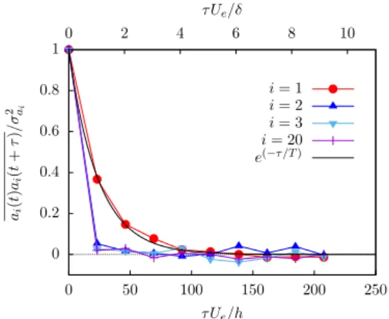
by Towne et al. (2018) and demonstrated by Mendez et al. (2018), the classical POD, while allowing for the best con-vergence, is not able to properly account for the dynamics of different coherent structures of similar energy, therefore, producing spectral mixing of different phenomena over different modes. Moreover, the PIV is by nature a method that samples the flow producing discrete time information without the possibility of implementing an analog low-pass filter prior digitization. Therefore, from a temporal point of view, when the acquisition frequency of the PIV system is low compared to the entire spectral content of the flow, the classical spectral aliasing phenomenon (in the temporal domain) is expected to occur. In the present case, given the low PIV sampling frequency of 5 Hz (and even if it is higher than the typical frequency of the most energetic structures in the boundary layer, see Fig. 3), only the first POD mode appears to bear the footprint of the low-frequency large-scale energetic LSMs of the boundary layer. This is shown in Fig. 4 where the auto-correlation function of the first tem-poral POD coefficients ai(t) (see Sect. 2.3.1 for a complete
definition) computed from the SPIV data is reported. As can be seen, only the auto-correlation of the first temporal mode is well resolved. The latter is well approximated by an exponential decaying function of the form e(−𝜏∕T) with T the
integral timescale which, when Taylor’s hypothesis is used, can be related to a characteristic length scale Lx≈ 24h or
1.05𝛿 , confirming that the first mode is associated with large-scale motion. Yet, the spatio-temporal dynamics of these LSMs is richer than what can be represented by one single mode and is, therefore, not correctly captured. To overcome
(b) (a) 0 2 4 6 8 10 12 14 16 100 101 102 1030 2 4 6 8 10 12 14 16 σ 2 u/u 2 τ u (z )/u τ (z − d)/z0 HWA PIV 10−2 10−1 100 101 102 103 100 101 102 z = h f. δ/ u (z ) (z − d)/z0 f.Suu(f )/u 2 τ fs/2
Fig. 3 Statistics of the streamwise velocity u. a Profiles of mean and
variance obtained by (red open circles) PIV and (gray open squares) hot-wire anemometry at the same streamwise location (1h down-stream the updown-stream cube). Light red-shaded areas represent the sta-tistical errors of the PIV statistics with a 95% confidence level. Sta-tistical errors for the HWA measurements being below 1% are not
shown. The solid black line shows the logarithmic law of Eq. (1). b Pre-multiplied spectra f .Suu(f )∕u
2
𝜏 (gray contours, shown with an
increment of 0.08, from 0.08 to 0.88). Blue filled circles indicate the local maxima of the pre-multiplied spectra; the thick solid green line shows the Nyquist frequency fs∕2 associated with the low-rate PIV
this limitation, a modification of the snapshot POD is pro-posed based on the recent results of Sieber et al. (2016). In the new method, the POD kernel is computed so as to take into account the long-term temporal coherence of the largest scales. This modified POD approach enables the de-aliasing of the first POD modes which will be shown to bear all the characteristics of the LSMs identified in the current litera-ture. Such an approach has been formalized by Sieber et al. (2016). The authors refer to this POD method as spectral POD as they showed that it behaves as a band-pass filter in the frequency domain. It must be noted that this variant of POD is different from the space-time formulation of POD originally proposed by Lumley (1967), which involves the decomposition of the cross-spectral density tensor and has hence later been referred to as spectral POD as well.
2.3.1 Classical snapshot POD
Lumley (1967) first proposed the POD technique to identify the coherent structures in turbulent flows. When limited to space only, it consists in extracting from the flow the struc-ture 𝜙(X) with the largest mean-square projection onto the fluctuating velocity field u�(X, t) over the spatial domain of
interest. This maximization problem leads to the solving of an integral problem of eigenvalues. It allows for the decom-position of the fluctuating velocity field u′ into a set of
tem-poral and spatial orthogonal modes ai(t) and 𝜙i(X) such that,
in the most general case,
In the present work, with the PIV data being well resolved in space but with a limited number of time samples, the snap-shot POD proposed by Sirovich (1987) has been employed.
(3) u�(X, t) = ∞ ∑ i=1 ai(t) 𝜙i(X).
The number of PIV snapshots (or time steps) is denoted N. In that case, the integral eigenvalue problem to solve is
where 𝜆i is the ith eigenvalue which represents the turbulent
energy contained in the ith mode. The matrix R ∈ N×N
defines the temporal cross-correlation matrix (or kernel) whose elements (i, j) are computed as
where V is the spatial domain over which the measurements have been performed. The temporal eigenvectors ai are
uncorrelated in time:
while the spatial modes are orthonormal and computed by
2.3.2 Spectral POD
Sieber et al. (2016) have recently introduced a modification of the temporal correlation matrix R originally used in the conventional snapshot POD to include an additional temporal constraint that enables a clear separation of phenomena that occur at multiple frequencies and energies. They proposed to apply a low-pass filter g along the diagonals of R to augment its diagonal similarity. A new temporal correlation matrix S is obtained by first integrating the velocity product over the spatial domain V and then by applying the filter temporal func-tion g:
The function g is a symmetric finite impulse response filter of width 2Nf+1 . In the simplest case, g would be a box filter
of value 1∕(2Nf+ 1) for k ∈ [−Nf; Nf] , and zero elsewhere.
As discussed by Sieber et al. (2016), a Gaussian filter can be employed to obtain a smooth response in time and frequency domaind. The eigenvalue problem to solve becomes
where 𝜇i is the eigenvalue of the temporal S-POD mode bi .
The modes b are orthogonal (i.e. uncorrelated in time): (4) Rai= 𝜆iai, (5) Rij= 1 N ∫V u�(X, ti)u � (X, tj)dV, (6) a iaj=ai(t)aj(t) = 1 N N ∑ k=1 ai(tk)aj(tk) = 𝜆i𝛿 ij, (7) 𝜙i(X) = 1 𝜆i aiu�(X). (8) Sij= 1 N Nf ∑ k=−Nf ∫V gku�(X, ti+k)u�(X, tj+k)dV. (9) Sbi= 𝜇ibi; 𝜇1≥ 𝜇2≥ ⋯ ≥ 𝜇N, (10) bibj= 𝜇i𝛿ij. 0 0.2 0.4 0.6 0.8 1 0 50 100 150 200 250 0 2 4 6 8 10 ai (t )ai (t + τ )/σ 2 ai τ Ue/h τ Ue/δ i = 1 i = 2 i = 3 i = 20 e(−τ /T )
Fig. 4 Normalized temporal auto-correlation function of the classical
snapshot POD temporal modes ai(t) as defined in Eq. 3, for i = 1 , 2, 3
In contrast to Sieber et al. (2016), the temporal S-POD modes are now projected onto time-delayed fluctuating velocity fields to obtain spatio-temporal S-POD modes:
The index k ∈ [−Nf; Nf] corresponds to a time delay
𝜏
k= k∕fs∈ [−Tf; Tf] , where Tf = Nf∕fs is the half-width of
the filter function g . For the sake of brevity, the modes 𝜳i
are referred to as spatial modes in the following. These spa-tial S-POD modes are orthonormal if the following inner product is employed:
It must be noted here that the present definition of the spa-tial S-POD modes is different from that proposed by Sieber et al. (2016). These authors indeed originally defined these modes as being dependent on space only by not including the integration over the temporal span of the low-pass filter in Eq. 12. As mentioned by Sieber et al. (2016), the modes are not orthogonal if defined in this manner. Therefore, by including their dependence on the time delay 𝜏 , the present modified definition of the modes 𝜳 leads to orthonormal modes, in agreement with the original POD approach. The original velocity field can be reconstructed by considering the spatio-temporal modes at zero time as
The definition of the spatio-temporal modes proposed here does not alter any other property of the spectral POD as designed by Sieber et al. (2016). As shown by Eq. 8, the S-POD acts as a band-pass filter centered around the domi-nant frequency, whose half-width Tf is controlled by the
characteristics of the low-pass filter g(𝜏) . Given the value of Nf , two asymptotic cases exist: if Nf= 0 , the S-POD is equivalent to the conventional POD, while for Nf= +∞ , it corresponds to the discrete Fourier transform. To benefit from the band-pass filtering effect of the S-POD, Sieber et al. (2016) advise to choose a value of Nf so that the filter half-width Tf corresponds to two to three times the
charac-teristic timescale of the phenomena of interest. In the present study, a Gaussian filter is used for g. The most energetic frequencies in the outer region are of the order f 𝛿∕u(z) ≈ 0.3 (Fig. 3b). In the upper region of the SPIV field of view, this corresponds to frequencies of approximately 1 Hz. Given the acquisition frequency of the PIV system of fs= 5 Hz,
N
f should be equal to 15 to ensure that the filter width spans
(11) 𝜳i(X, 𝜏k) = 1 𝜇i N−k ∑ l=1+k bi(tl)u�(X, t l+k). (12) Nf ∑ k=−Nf 1 V ∫V𝜳i(X, 𝜏k)𝜳j(X, 𝜏k)dV = 𝛿ij. (13) u(X, t) = ̄u(X) + N ∑ i=1 bi(t)𝜳i(X, 𝜏 = 0).
three times this characteristic timescale. In the following, it is shown that a value of Nf= 16 leads to satisfactory results in terms of large-scale extraction.
3 Results
Both the conventional (i.e. Nf = 0 ) and spectral snapshot POD detailed previously are now employed. Only the streamwise velocity component u is considered. The spatial eigenvectors 𝜙 and 𝜳 are function of the streamwise x and wall-normal z coordinates. Using S-POD, the fluctuations of the streamwise velocity component u are then decomposed into u�= u�
L+ u �
S , where u′S is the small-scale component of
u′ and u′
L the large-scale component defined as
where NPOD is the number of POD modes selected to define
the large-scale component. 3.1 S‑POD analysis
In the following, most of the results correspond to the case Nf= 16 , the value for which the low-pass filter width T
f is
equal to three times the characteristic timescale of the phe-nomena of interest. While a systematic study of the effect of Nf on the results has been performed, it is not reported here for conciseness. As described by Sieber et al. (2016) in detail, the influence of varying Nf can be directly seen on the frequency content of the temporal S-POD coefficients bi(t) . The S-POD acts as a band-pass filter applied to the bi(t) , the width (in the frequency domain) of which vary-ing from +∞ ( Nf= 0 , equivalent to the classical POD) to the narrowest possible one, dictated by the PIV sampling of the flow ( Nf = +∞ , equivalent to the Fourier transform). The frequency around which the band-pass filter is applied is intrinsically selected by the S-POD, based on the ener-getic optimality criterion underpinning POD. The choice of Nf results in a compromise between the fastest energetic convergence (POD) and the best frequency resolution (Fou-rier decomposition). This is effect is readily visible on the eigenspectrum.
As mentioned earlier, given the low acquisition fre-quency fs and the limited field of view of the employed
SPIV system, a major drawback of the conventional snap-shot POD (i.e. Nf = 0 ) is the spectral mixing of different
coherent structures over different modes and the aliasing of the low-order modes by the smaller scales. These most energetic modes which should correspond to slow-varying large scales of the present boundary layer do not present (14) u� L(x, z) = NPOD ∑ i=1 bi(t)𝛹i(x, z, 𝜏 = 0),
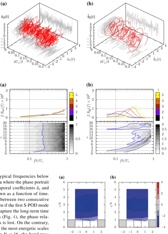
a smooth time evolution with typical frequencies below fs∕2 . This is illustrated in Fig. 5a where the phase portrait
of the first two normalized temporal coefficients ̃a1 and
̃a2 and their time traces are shown as a function of time.
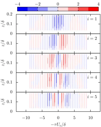
No apparent continuity in time between two consecutive samples is visible. Therefore, even if the first S-POD mode obtained with Nf= 0 is able to capture the long-term time correlation of the largest scales (Fig. 4), the phase rela-tionship with subsequent modes is lost. On the contrary, when the temporal coherence of the most energetic scales is taken into account by setting Nf= 16 , the band-pass filtering effect of S-POD allows for the proper time resolu-tion of the first S-POD modes (Fig. 5b). This is confirmed by the computation of the pre-multiplied energy spec-tra of the normalized temporal coefficients ̃ai and ̃bi , for i∈ [1∶20] (Fig. 6). When Nf= 0 , all the temporal modes show an accumulation of energy at high frequency with-out a clear well-defined spectral content, which is typical of the aliasing phenomena (Fig. 6a). Conversely, setting Nf= 16 leads to a clear band-pass filtering of the energy content (Fig. 6b). The energy of the first S-POD modes is clearly contained in a limited frequency band, the cor-responding most energetic frequency increasing with the
order of the mode i. When i > 5 , a secondary peak at lower frequency appears, which can be attributed again to alias-ing. Therefore, with the present SPIV setup, the use of S-POD with the proper filter width (set in accordance with the characteristic frequencies of the most energetic struc-tures existing in the outer of the boundary layer) allows for the de-aliasing of the largest scales (here limited to i ≤ 5).
Fig. 5 Phase portrait of the
first two normalized temporal S-POD coefficients of u for a
Nf= 0 ( ̃ai= ai∕√𝜆i ) and b Nf= 16 ( b̃i= bi∕√𝜇i)
(b)
(a)
0 0.05 0.1 0.15 0.2 0.25 0.3−4−3 −2−1 0 1 2 3 4 −4 −3 −2 −1 0 1 2 3 4 ˜ a2(t) tUc/δ ˜ a1(t) ˜ a2(t) 0 0.05 0.1 0.15 0.2 0.25 0.3−4−3 −2−1 0 1 2 3 4 −4 −3 −2 −1 0 1 2 3 4 ˜b2(t) tUc/δ ˜b1(t) ˜b2(t)Fig. 6 Pre-multiplied spectra
of temporal S-POD normalized coefficients for a Nf= 0 and
b Nf= 16 . The upper part of
the plot shows pre-multiplied spectra of the first five temporal S-POD coefficients (colored by the mode order i), the bottom part the pre-multiplied spectra contours in shades of gray for the first 20 modes. The solid blue line shows the 0.25 contour
(b)
(a)
0 1 2 3 0.1f δ/U 1 c 0 2 4 6 8 10 12 14 16 18 20 i 0 0.5 1 f. S˜a ˜a (f ) × 10 3 1 2 3 4 5 i 0 1 2 3 0.1 f δ/U 1 c 0 2 4 6 8 10 12 14 16 18 20 i 0 0.5 1 1.5 2 2.5 3 f. S˜ b˜b (f ) × 10 3 1 2 3 4 5 i −2 −1 0 1 2 x/h 0 1 2 3 4 5 6 z/ h −2 −1 0 1 2 x/h 0 1 2 3 4 5 6 z/ h −4 −2 0 2 4 (b) (a)Fig. 7 First spatial S-POD modes 𝛹i(x, z, 𝜏 = 0) of u with a Nf= 0 and b Nf= 16
When analyzing the spatial structures of the first S-POD mode, the influence of the filter width is not that obvious. The first eigenvectors of the POD and S-POD (for 𝜏 = 0 ) are shown in Fig. 7. In both cases, the first spatial modes obtained are very similar and correspond to the occurrence of high- (or low-)speed events in the flow spanning the whole region z > 1.5h.
However, using S-POD with Nf ≠ 0 leads to
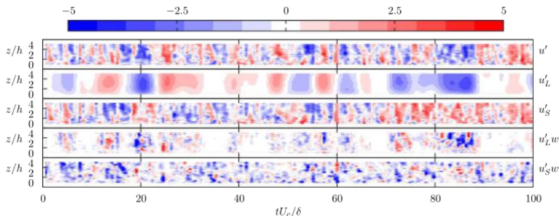
spatio-tempo-ral modes 𝛹 (x, z,𝜏) which bear the imprint of the long-term coherence of the large most energetic scales of the flow. The first five S-POD modes obtained with Nf= 16 are shown in
Fig. 8. To represent the spatio-temporal structure of the S-POD modes, Taylor’s approximation is here used to transform the time delay 𝜏 in a pseudo-streamwise spatial coordinate with an advection velocity Uc corresponding to the average mean
velocity across the measurement region. Estimating the actual convection velocity of the large-scale coherent structures, which is known to be a function of the wall-normal distance and the considered scale (Dennis and Nickels 2008), is out of the scope of the present study and not further investigated. Even if Taylor’s approximation is known to have limitations in the region of spatial heterogeneity and high level of turbulence intensity, it is employed here for the sake of displaying the
spatio-temporal structure of the S-POD modes 𝛹 (x, z,𝜏) . The size of each colored strip in Fig. 8 corresponds to that of the SPIV field of view. Each mode depicts an oscillatory behavior along the temporal direction, the typical scale of which being of the order of several boundary layer height 𝛿 . This character-istic is in perfect agreement with that of the VLSMs evidenced in boundary layer flows using more conventional techniques (Guala et al. 2011; Hutchins and Marusic 2007). The higher the mode order, the smaller its time period, in agreement with the fact that higher order modes usually correspond to smaller scales, in particular when one direction of analysis of the flow corresponds to the direction of advection of the flow (stream-wise and time directions here). Limiting the frequency content of the S-POD modes by setting Nf > 0 has, however, an effect
on the energy content of each mode and on the rate of con-vergence of the POD decomposition in terms of number of modes required to represent a given amount of kinetic energy. The larger the Nf , the slower the convergence, the energy con-tent of each mode being constrained by the band-pass effect of the S-POD method (Fig. 9). Using Eq. 14, the large-scale streamwise velocity component u′
L corresponding to the
con-tribution of the first Nf S-POD modes can be reconstructed. In the present case, NPOD is set to five, the number of S-POD
modes properly resolved in time by the S-POD when using Nf= 16 . The small-scale streamwise velocity component u′
S
is calculated as u�
S= u�− u�L . An example of the temporal
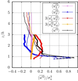
evolution of the instantaneous streamwise velocity compo-nent fluctuation, its large- and small-scale compocompo-nents and their contribution to the shear-stress u�
w�= u� Lw �+ u� Sw � is shown in Fig. 10. Despite the low PIV acquisition frequency, the temporal evolution of u′ clearly shows the footprint of
large-scale coherent structures with typical time period of a few timescale 𝛿∕Uc . The time series of u
′ L exhibits alternation i = 5 i = 4 i = 3 i = 2 i = 1 −10 −5 0 5 10 −τ Uc/ 0 0.1 z/ 0 0.1 z/ 0 0.1 z/ 0 0.1 z/ 0 0.1 0.2 z/ −4 −2 0 2 4
Fig. 8 First five spatial S-POD modes 𝛹 (x, z,𝜏) of u with Nf= 16 . The size of each colored strip corresponds to that of the SPIV field of view 0 0.2 0.4 0.6 0.8 1 1 10 100 1000 Nf= 0 Nf= 20 NPO D k =1 λk / N k=1 λk NP OD Nf= 0 Nf= 16
Fig. 9 Energy contribution of the first NPOD S-POD modes of u as a
function of the filter size Nf . Results are shown for Nf= 0 to 20 with an increment of 2. The dashed black line with crosses shows the case
Nf= 0 corresponding to the conventional snapshot POD, the solid red line with open circles shows the Nf= 16 case. The red plus sign ( + ) corresponds to Nf= 16 , NPOD= 5
of low- and high-momentum regions with typical time period of the order of at least 10 𝛿∕Uc and spanning the entire
wall-normal extent of the PIV field of view. The coherent structures represented by the first NPOD= 5 S-POD modes, therefore, show the typical features of boundary layer VLSMs. The com-ponent u′
S also shows some smaller timescale organization, less
coherent in the wall-normal direction, consistent l with the presence of LSMs embedded into the VLSMs. This is sup-ported by the analysis of the instantaneous decomposed shear stress that shows the presence of smaller scale shear stress events, in agreement with the hairpin-vortex packet model (Adrian 2007). The pre-multiplied spectra of u′
L are shown
in Fig. 11a as a function of the wall-normal coordinate (red contours) and are compared to that obtained with conventional
HWA. First, as expected from the above analysis, they do not show any trace of aliasing at high frequency, as if the original velocity field had been properly low-pass filtered. Second, the frequency of the maximum of energy in the upper part of the SPIV measurement region (i.e. (z − d)∕z0> 20 ) corresponds
well to that of the most energetic structures found in the outer region of the boundary layer by Perret et al. (2019). Again, a good agreement of the energy ridge of the pre-multiplied spectra of u′
L with the most energetic frequency of the large
scales extracted by Perret et al. (2019) is observed across the entire measurement region. Moreover, the present analysis shows that the most energetic (large) scales from the outer layer reach deep into the roughness sublayer, being superim-posed onto the smaller scales. The contribution of u′
L to the
Fig. 10 Example of the
tem-poral evolution of (from top to bottom) u′ , u′
L , u′S , u′Lw′ and u′Sw′
measured at fs= 5 Hz on the centerline of the PIV field of view (all quantities normalized by u𝜏 ). The horizontal dotted
black lines indicate to z = h
uSw uLw uS uL u 0 20 40 60 80 100 tUc/δ 0 2 4 z/h 0 2 4 z/h 0 2 4 z/h 0 2 4 z/h 0 2 4 z/h −5 −2.5 0 2.5 5 (a) (b) 10−2 10−1 100 101 102 103 100 101 102 z = h f. δ/ u (z ) (z − d)/z0 S-POD HWA 0 1 2 3 4 5 6 0 0.2 0.4 0.6 0.8 1 z/ h σ2 uL/σ 2 u, uLw / u w σ2 uL uLw
Fig. 11 a Wall-normal evolution of the pre-multiplied spectra
f .SuLuL(f )∕u
2
𝜏 of the large-scale streamwise velocity component u
′ L
reconstructed with NPOD= 5 ( Nf= 16 ) (red solid lines, shown with an increment of 0.04, from 0.04 to 0.44). As in Fig. 3, solid gray lines (shown with an increment of 0.08, from 0.08 to 0.88) corre-spond to pre-multiplied spectra of u′ as measured via HWA by
Per-ret et al. (2019), blue filled circles indicate the local maxima of these pre-multiplied spectra; the thick solid green line shows the Nyquist frequency fs∕2 associated to the present low-rate PIV system. Solid
black triangles show the most energetic frequency corresponding to
the large scales identified by Perret et al. (2019) via their two-point spectral analysis. b Contribution of the first five S-POD modes to
𝜎2
u and ⟨u
′w′⟩ . Red solid line: 𝜎2
u of the present study, green dashed
line: ⟨u′w′⟩ of the present study. Red symbol: results for 𝜎2
u L . Filled and open squares correspond to the results of Perret et al. (2019) and Blackman and Perret (2016), respectively. Filled triangles correspond to 𝜎2
u
L obtained using a frequency cutoff ( fc ) as in Mathis et al. (2009) with fc= 0.3Ue∕𝛿 applied to the present HWA data. Green open
total velocity variance 𝜎2
u and the Reynolds shear stress ⟨u
′w′⟩ is shown in Fig. 11b. The extracted large scales using the first S-POD modes are found to be contributors to both the Reyn-olds shear stress and the variance of the streamwise veloc-ity component above the roughness sublayer (i.e. z ≳ 2h ) as already observed in flows over urban canopies (Castro et al.
2006; Coceal et al. 2007). Comparison with the results from Blackman and Perret (2016) and Perret et al. (2019) obtained in the same flow configuration shows a relatively good quali-tative agreement given the different methods employed to extract the large-scale component from u′ in the three studies.
Blackman and Perret (2016) indeed used a multi-time delay stochastic estimation-based method to extract u′
L from
synchro-nized SPIV and HWA measurements while Perret et al. (2019) employed two-point single HWA measurements to extract the part of u�(z) the most correlatedwith u�(z∕h = 5) measured by
a fixed reference probe (the reader is referred to their work for a complete description of the corresponding methods and results). For the sake of completeness, the method of Mathis et al. (2009) to extract uL using a sharp low-pass filter in the spectral domain is applied to the present HWA data (red trian-gles in Fig. 11b). The cutoff frequency is set to fc= 0.3Ue∕𝛿
following the analysis of Basley et al. (2018) of the same flow configuration. The overall agreement with the S-POD method is good, in particular for z∕h > 2 . Closer to the canopy, the discrepancy is larger, probably due to the presence of can-opy-produced energetic coherent structures superimposed on boundary layer large scales (Perret et al. 2019).
The effectiveness of the scale separation obtained pres-ently motivate further investigation to identify the nature of the interactions between the canopy scales and those from the incoming boundary layer, as detailed below.
3.2 Scale interaction
An analysis of the interaction of these large-scale structures with the smaller scale turbulence is presented here. The emphasis is on the existence of the non-linear interaction that resembles an amplitude modulation mechanism that has been shown to exist in smooth-wall flow (Mathis et al.
2011) but also in flow over urban-like roughness (Anderson
2016; Basley et al. 2018; Blackman and Perret 2016). The third-order moment of the streamwise velocity component can be written as
where u′
S is the small-scale component of u′ and u′L the
large-scale component such that u�
= u�
L+ u �
S . Mathis et al. (2011)
used the same type of decomposition in their study of a flat plate turbulent boundary layer and showed that the cross-term 3⟨u′
Lu′2S⟩ is directly linked to the existence of a
mecha-nism of amplitude modulation of the near-wall turbulence (15) ⟨u�3⟩ = ⟨u�3 L⟩ + 3⟨u �2 Lu � S⟩ + 3⟨u � Lu �2 S⟩ + ⟨u �3 S⟩,
by the larger scales. The above results have demonstrated that the present decomposition method (even if based on an energetic criterion) has allowed for the identification of the known VLSMs existing in boundary layer flows. Therefore, ⟨u′
Lu′2S⟩ can be viewed as the indicator of interaction between
the identified structures and the remaining of the flow (of smaller scale). Even if the term ⟨u′
Lu′2S⟩ does not allow for a
precise quantification of the magnitude and the direction of the mean energy transfers, its non-zero value demonstrates the existence of non-linear interactions between scales (Blackman et al. 2018a). The contribution of the large-scale component to the skewness of the streamwise velocity component is shown in Fig. 12. While the skewness of the large-scale part ⟨u′3
L⟩ is found to be almost zero in the entire
domain, the skewness of the small-scale component ⟨u′3 S⟩ is,
in contrast, a non-negligible contributor to the total skew-ness of the streamwise velocity fluctuations in the roughskew-ness sublayer (i.e. z∕h < 3 ). It is noticeable that the evolution of this term with the wall-normal distance is very similar to the evolution of the skewness of the streamwise velocity across a mixing layer in which positive values are found in the low-speed region and negative values on the high-speed side of the shear-layer (Druault et al. 2005). This may sug-gest that once the influence of the larsug-gest scales is removed, the roughness-sublayer flow behaves as a shear layer flow. This is consistent with what has been observed in boundary layer flows over vegetation canopy (Finnigan 2000). The investigation of this point will be addressed in future work. The terms ⟨u′
Lu′2S⟩ and ⟨u′2Lu′S⟩ representing non-linear
inter-actions between the large and small scales are also found to contribute largely to the skewness. The importance of these two terms indicates that the large and small scales are phase-coupled through a mechanism that resembles an amplitude
z/ h u3 /σ3 u u3 L u3 S 3 uLu2 S 3 u2 LuS u3 0 1 2 3 4 5 6 −0.4 −0.2 0 0.2 0.4 0.6 0.8 1
Fig. 12 Scale-decomposed skewness of the streamwise velocity
com-ponent of (lines) the present study and (symbols) Blackman and Per-ret (2016) (all terms normalized by 𝜎3u∕2)
modulation mechanism as found by Mathis et al. (2009) in smooth-wall boundary layers. For the sake of completeness, the present results are compared with those from Blackman and Perret (2016) obtained in the same flow configuration (symbols in Fig. 12). As mentioned above, given the dif-ference between the employed methods to extract the large scales from the raw u′ component and the extent of the SPIV
measurement regions, the agreement is fairly good, demon-strating the relevance of the present S-POD approach to per-form scale decomposition and to identify scale-interaction mechanisms.
Finally, the spectral decomposition of the term ⟨u′ Lu′2S⟩ ,
which bears the footprint of the amplitude modulation mech-anism is analyzed. The present S-POD analysis gives access to time-resolved large-scale signals and, therefore, allows for cross-spectral analysis of u′
L and u′2S . Computing the spectral
coherence between these two signals is equivalent to the analysis as a function of frequency of the correlation coef-ficient between u′
L and the large-scale envelope of u′S . The
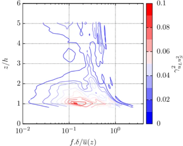
coherence map between u′
L and u′2S is shown in Fig. 13 as a
function of both the frequency and the wall-normal distance z. While the coherence level is below ≈ 0.1 , a maximum is manifest for z∕h ≈ 1 and f 𝛿∕u(z) ≈ 0.15 indicating that the large scales modulate the large-scale component of the enve-lope of the small-scale time history as also found by Mathis et al. (2009) for smooth-wall configurations. While not reported here for conciseness, the phase of the cross-spec-trum is non-zero. This confirms that the maximum of ampli-tude modulation occurs with a time delay between the large and the small scales, in agreement with the finding of Black-man and Perret (2016) and Guala et al. (2011), for instance. In addition, it must be noted that when the interaction between uL and the spanwise or the wall-normal components v or w, respectively, is considered (Fig. 14), the profiles of 3⟨u′
Lu′2j ⟩ , j = 2 or 3, are qualitatively similar to that of
3⟨u′
Lu′2S⟩ . Even if the scales of w and v involved in these
cross-terms remain to be identified, it suggests that in the roughness sublayer, the low- and high-speed structures of largest scales interact with structures involving the three components of the velocity through the same type of non-linear mechanisms.
4 Conclusions
A high-Reynolds number boundary layer flow developing over large roughness elements representative of the urban canopy has been investigated via the use of the recently introduced spectral POD (Sieber et al. 2016). It has been demonstrated that this approach, which acts as a band-pass filtering operation on the temporal coefficients obtained from the conventional snapshot POD, enables to account for the long-term coherence of the most energetic large-scale structures existing in the outer layer of the boundary layer. When applied to stereoscopic PIV velocity fields that are of limited extent in the streamwise direction and which have been acquired with a sampling frequency too low to properly capture the spectral content of the flow, S-POD proved to be able to extract the large-scale coher-ent structures from the flow via the proper choice of the filter width. In the present case, the use of the S-POD can be viewed as augmenting the snapshot POD kernel by extending the database in the streamwise direction through the use of Taylor’s approximation. This case would cor-respond to the use of a simple low-pass box filter. A modi-fication of the definition of the spatial S-POD modes has been proposed so that they are orthonormal to each other.
0 1 2 3 4 5 6 10−2 10−1 100 z/ h f.δ/u(z) 0 0.02 0.04 0.06 0.08 0.1 γ 2 uL u 2 S
Fig. 13 Spectral coherence between the large scales u′ L and u
′2 S as a
function of the wall-normal location
0 1 2 3 4 5 6 −0.4 −0.2 0 0.2 0.4 0.6 0.8 1 z/ h 3 uLx2 /(σuσ2 x) 3 uLu2 S 3 uLv2 3 uLw2
Fig. 14 Third-order moments 3⟨u′ Lu ′2 S⟩ , 3⟨u ′ Lv′2⟩ and 3⟨u ′ Lw′2⟩ (all terms normalized by 𝜎u𝜎 2 {u,v,w})
It results in spatio-temporal modes which reflect the sta-tistical organization of the most energetic structures both in space and time.
The characteristics of the educed large-scale coherent structures have been shown to correspond well to that of the VLSMs identified in the turbulent boundary layer in the literature. In agreement with previous work in similar flow configurations, the large scales extracted via S-POD have been found to consist of elongated low- or high-momentum regions. They are major contributors to the turbulent kinetic energy and the Reynolds shear stress in the outer region of the flow. The extracted large-scale structures were shown to interact with small-scale near-wall turbulence through a mechanism of both superimposition and amplitude modula-tion. The three velocity components were found to be under the influence of the large-scale component of the streamwise velocity component, in agreement with recent findings in smooth- and rough-wall boundary layers (Talluru et al. 2014; Blackman and Perret 2016).
Acknowledgements The authors would like to thank Dr. Cédric Rivet
for providing the SPIV data and Mr Thibaut Piquet for his technical support during the experimental program. The authors also acknowl-edge the financial support of the French National Research Agency through the research Grant URBANTURB no. ANR-14-CE22-0012-01.
References
Adrian RJ (2007) Hairpin vortex organization in wall turbulence. Phys Fluids 19(4):041301. https ://doi.org/10.1063/1.27175 27 Anderson W (2016) Amplitude modulation of streamwise velocity
fluctuations in the roughness sublayer: evidence from large-eddy simulations. J Fluid Mech 789:567–588
Basley J, Perret L, Mathis R (2018) Spatial modulations of kinetic energy in the roughness sublayer. J Fluid Mech 850:584–610 Blackman K, Perret L (2016) Non-linear interactions in a boundary
layer developing over an array of cubes using stochastic estima-tion. Phys Fluids 28(095):108
Blackman K, Perret L, Calmet I, Rivet C (2017) Turbulent kinetic energy budget in the boundary layer developing over an urban-like rough wall using PIV. Phys Fluids 29(085):113
Blackman K, Perret L, Calmet I (2018a) Energy transfer and non-linear interactions in an urban boundary layer using stochastic estima-tion. J Turb 19(10):849–867
Blackman K, Perret L, Savory E (2018b) Effect of upstream flow regime and canyon aspect ratio on non-linear interactions between a street canyon flow and the overlying boundary layer. Bound-Layer Meteorol 169(3):537–558
Calluaud D, David L (2004) Stereoscopic particle image velocimetry measurements of the flow around a surface-mounted block. Exp Fluids 36(1):53–61
Castro IP (2007) Rough-wall boundary layers: mean flow universality. J Fluid Mech 585:469–485
Castro IP, Cheng H, Reynolds R (2006) Turbulence over urban-type roughness: deductions from wind-tunnel measurements. Bound-Layer Meteorol 118:109–131
Cheng H, Hayden P, Robins AG (2007) Flow over cube arrays of dif-ferent packing densities. J Wind Eng Ind Aerodyn 95:715–740
Coceal O, Dobre A, Thomas TG (2007) Unsteady dynamics and organ-ized structures from DNS over an idealorgan-ized building canopy. Int J Climatol 27:1943–1953
del Alamo JC, Jimenez J (2003) Spectra of the very large anisotropic scales in turbulent channels. Phys Fluids 15:41–44
Dennis DJC, Nickels TB (2008) On the limitations of taylor’s hypoth-esis in constructing long structures in a turbulent boundary layer. J Fluid Mech 614:197–206. https ://doi.org/10.1017/S0022 11200 80033 52
Druault P, Delville J, Bonnet J (2005) Experimental 3D analysis of the large scale behaviour of a plane turbulent mixing layer. Flow Turbul Combust 74(2):207–233
Finnigan JJ (2000) Turbulence in plant canopies. Annu Rev Fluid Mech 32:519–571
Grimmond CSB, Oke TR (1999) Aerodynamic properties of urban areas derived from analysis of surface form. J Appl Meteorol 38:1262–1292
Guala M, Metzger M, McKeon BJ (2011) Interactions within the tur-bulent boundary layer at high reynolds number. J Fluid Mech 666:573–604
Herpin S, Perret L, Mathis R, Tanguy C, Lasserre JJ (2018) Inves-tigation of the flow inside an urban canopy immersed into an atmospheric boundary layer using Laser Doppler anemometry. Exp Fluids 59:80–103
Hultmark M, Smits AJ (2010) Temperature corrections for constant temperature and constant current hot-wire anemometers. Meas Sci Technol 21:1–4
Hutchins N, Marusic I (2007) Evidence of very long meandering fea-tures in the logarithmic region of turbulent boundary layers. J Fluid Mech 579:1–28
Hutchins N, Chauhan K, Marusic I, Monty J, Klewicki J (2012) Towards reconciling the large-scale structure of turbulent bound-ary layers in the atmosphere and laboratory. Bound-Layer Mete-orol 145(2):273–306
Inagaki A, Kanda M (2010) Organized structure of active turbulence over an array of cubes within the logarithmic layer of atmospheric flow. Bound-Layer Meteorol 135:209–228
Jackson PS (1981) On the displacement height in the logarithmic veloc-ity profile. J Fluid Mech 111:15–25
Jimenez J (2004) Turbulent flows over rough walls. Annu Rev Fluid Mech 36:173–196
Lumley JL (1967) The structure of inhomogeneous turbulent flows. In: Yaglom AM, Tatarski VI (eds) Atmospheric turbulence and radio propagation. Nauka, Moscow, pp 166–178
Marusic I, Hutchins N (2008) Study of the log-layer structure in wall turbulence over a very large range of Reynolds number. Flow Turbul Combust 81:115–130
Mathis R, Hutchins N, Marusic I (2009) Large-scale amplitude modu-lation of the small-scale structures in turbulent boundary layers. J Fluid Mech 628:311–337
Mathis R, Hutchins N, Marusic I, Sreenivasan KR (2011) The relation-ship between the velocity skewness and the amplitude modulation of the small scale by the large scale in turbulent boundary layers. Phys Fluids 23:1–4
Mendez MA, Balabane M, Buchlin JM (2018) Multi-scale proper orthogonal decomposition of complex fluid flows. arXiv e-prints arXiv :1804.09646 , arXiv :1804.09646
Monty JP, Stewart JA, Williams RC, Chong MS (2007) Large-scale features in turbulent pipe and channel flows. J Fluid Mech 589:147–156
Perret L, Rivet C (2018) A priori analysis of the performance of cross hot-wire probes in a rough wall boundary layer based on stereo-scopic PIV. Exp Fluids 59(10):153
Perret L, Savory E (2013) Large-scale structures over a single street canyon immersed in an urban-type boundary layer. Bound-Layer Meteorol 148:111–131
Perret L, Basley J, Mathis R, Piquet T (2019) The atmospheric bound-ary layer over urban-like terrain: Influence of the plan density on roughness sublayer dynamics. Bound-Layer Meteorol 170(2):205– 234. https ://doi.org/10.1007/s1054 6-018-0396-9
Placidi M, Ganapathisubramani B (2015) Effects of frontal and plan solidities on aerodynamic parameters and the roughness sublayer in turbulent boundary layers. J Fluid Mech 782:541–566 Rivet C, Perret L, Rosant JM (2012) Scale interactions in an
urban-like boundary layer: a wind tunnel study. In: 20th Symposium on boundary layers and turbulence, Boston, MA
Savory E, Perret L, Rivet C (2013) Modeling considerations for exam-ining the mean and unsteady flow in a simple urban-type street canyon. Meteorol Atmos Phys 121:1–16
Sieber M, Paschereit CO, Oberleithner K (2016) Spectral proper orthogonal decomposition. J Fluid Mech 792:798–828
Sirovich L (1987) Turbulence and the dynamics of coherent structures. Part I: coherent structures. Q Appl Math 45(3):561–571 Snyder WH, Castro IP (2002) The critical Reynolds number for
rough-wall boundary layers. J Wind Eng Ind Aerodyn 90:41–54 Soloff SM, Adrian RJ, Liu ZC (1997) Distortion compensation for
generalized stereoscopic particle image velocimetry. Meas Sci Technol 8(12):1441–1454
Takimoto H, Sato A, Barlow JF, Moriwaki R, Inagaki A, Onomura S, Kanda M (2011) Particle image velocimetry measurements of turbulent flow within outdoor and indoor urban scale models and flushing motions in urban canopy layers. Bound-Layer Meteorol 140:295–314
Talluru KM, Baidya R, Hutchins N, Marusic I (2014) Amplitude modu-lation of all three velocity components in turbulent boundary lay-ers. J Fluid Mech 746:R1. https ://doi.org/10.1017/jfm.2014.132 Towne A, Schmidt OT, Colonius T (2018) Spectral proper orthogonal
decomposition and its relationship to dynamic mode decomposi-tion and resolvent analysis. J Fluid Mech 847:821–867
Volino RJ, Schultz MP, Flack KA (2011) Turbulence structure in boundary layers over periodic two- and three-dimensional rough-ness. J Fluid Mech 676:172–190