Theory and identification of a constitutive model of induced anisotropy by the Mullins effect

HAL Id: hal-00958608

https://hal.archives-ouvertes.fr/hal-00958608

Submitted on 12 Mar 2014

HAL is a multi-disciplinary open access

archive for the deposit and dissemination of sci-entific research documents, whether they are pub-lished or not. The documents may come from teaching and research institutions in France or abroad, or from public or private research centers.

L’archive ouverte pluridisciplinaire HAL, est destinée au dépôt et à la diffusion de documents scientifiques de niveau recherche, publiés ou non, émanant des établissements d’enseignement et de recherche français ou étrangers, des laboratoires publics ou privés.

Theory and identification of a constitutive model of

induced anisotropy by the Mullins effect

Guilherme Machado, Grégory Chagnon, Denis Favier

To cite this version:

Guilherme Machado, Grégory Chagnon, Denis Favier. Theory and identification of a constitutive model of induced anisotropy by the Mullins effect. Journal of the Mechanics and Physics of Solids, Elsevier, 2014, 63, pp.29-39. �10.1016/j.jmps.2013.10.008�. �hal-00958608�

Theory and identification of a constitutive model of induced

1

anisotropy by the Mullins effect

2

G. Machado, G. Chagnon∗, D. Favier

3

UJF-Grenoble1, CNRS, TIMC-IMAG - UMR5525, Grenoble, France.

4

Abstract 5

Rubber-like materials present a stress softening phenomenon after a first loading known

6

as the Mullins effect. Some recent experimental data on filled silicone rubber is presented

7

in literature, using uniaxial and biaxial tests to precondition samples thus induce some

8

primary stress softening. A generic modeling based on the polymer network decomposition

9

into an isotropic hyperelastic one, and a stress-softening evolution one, is proposed taking

10

into account the contribution of many spatial directions. A new stress softening criterion

11

tensor is built by means of a tensor that measures the repartition of energy in space. A

12

general form of the stress softening function associated to a spatial direction is written by

13

the way of two variables: one, the maximal eigenvalue of the energy tensor; the other, the

14

energy in the considered direction. Finally, a particular form of constitutive equation is

15

proposed. The model is fitted and compared to experimental data. The capacities of such

16

modeling are finally discussed.

17

Key words: Mullins effect; stress-softening; strain-induced anisotropy; constitutive

18

equation

19

1. Introduction 20

Rubber-like materials present a stress softening after a first loading cycle, known as

21

the Mullins effect (Mullins, 1947). Different definitions have been given to the Mullins

22

effect, in this paper the Mullins effect is considered as the difference between the first

23

and second loadings. Moreover, different studies have highlighted that this phenomenon

24

induces anisotropy, since the stress softening is strongly dependent on the second load

25

direction.

26

∗_{Corresponding author}

In a first approach, many isotropic models were proposed in the literature to describe

27

stress softening. First, physical models taking into account the evolution of the chain

net-28

work were proposed. Govindjee and Simo (1991) proposed a model based on the

macro-29

molecular network evolution by decomposition into a hyperelastic network and an evolving

30

network. Marckmann et al. (2002) considered that the macromolecular network can be

31

represented by the eight chains model (Arruda and Boyce, 1993). The model containing

32

chain lengths and chain densities evolving with the maximal principal stretch. In another

33

way, double network theory was developed (Green and Tobolsky, 1946) considering that

34

the rubber-like material can be decomposed into a hard and a soft phase; the hard phase

35

is transformed into soft phase with the stress softening. Different equations were

pro-36

posed (Beatty and Krishnaswamy, 2000; Zu˜niga and Beatty, 2002). At the same time, the

37

damage theory was often used to describe the stress softening (Simo, 1987; Miehe, 1995;

38

Chagnon et al., 2004). In another way, Li et al. (2008) associated the Mullins effect to the

39

growth of cavities in the material and a compressible model was proposed. In a last point

40

of view, Ogden and Roxburgh (1999) and Dorfmann and Ogden (2003) proposed models

41

based on pseudo-elasticity. All these models fit experimental data more or less accurately

42

in one loading direction, i.e., without changing loading direction between first and second

43

loadings. For a more exhaustive review about these isotropic models, the reader can refer

44

to Diani et al. (2009).

45

To improve the modeling and to fit anisotropic stress softening, new approaches were

46

developed taking into account the difference of stress softening in each strain direction.

47

At first, G¨oktepe and Miehe (2005) generalized the approach proposed by Govindjee and

48

Simo (1991) taking into account a spatial repartition of the chains. In the same way,

49

Diani et al. (2006a) proposed a generalization of the Marckmann et al. (2002) model by

50

means of chains oriented into 42 or more directions in space. Using a phenomenological

51

damage function, this model can describe different stress softening in different directions,

52

with permanent deformation after unloading. Dargazany and Itskov (2009) proposed a

53

similar approach by taking into account the existence of different chains with different

54

lengths in each direction. They integrate the density of probability in each direction,

55

by taking into account the network evolution at each step. Shariff (2006) proposed an

56

anisotropic damage model that describes transverse anisotropy of Mullins effect, taking

57

into account different damages in the three principal strain directions using a second-order

damage tensor. In the same way, Itskov et al. (2010) proposed three damage evolution

59

functions for the three principal strain directions. These functions are formulated in terms

60

of material parameters that partly depend on the maximal principal stretch. Recently,

61

Dorfmann and Pancheri (2012) proposed a phenomenological model, based on the theory

62

of pseudo-elasticity, which includes scalar variables in the strain energy function to account

63

for stress softening and changes in material symmetry.

64

Most of the anisotropic models mentioned above are proposed by analyzing successive

65

tensile tests performed along different directions. In spite of that, Machado et al. (2012a)

66

has recently performed other original tests based on preconditioning with uniaxial tension

67

and biaxial tension tests. Based on Machado et al. (2012a) experimental results using

68

silicone rubber, this paper proposes a new approach for modeling the induced anisotropy

69

by the Mullins effect. In Section 2, the global framework of the Mullins effect modeling

70

is presented. In Section 3, a new approach is proposed to write constitutive equations by

71

introducing a tensor that describes the strain energy repartition in the space directions.

72

The conditions to be verified by the equations are detailed. In Section 4, a first constitutive

73

equation is proposed. It is fitted and compared to experimental data. Finally, Section 5

74

contains some concluding remarks and outlines some future perspectives.

75

2. Macromolecular approach to model Mullins effect 76

2.1. Filled silicone behavior

77

In the last few years, different tests highlighting the stress softening anisotropy have

78

been presented in the literature for different rubber-like materials, see for example (Muhr

79

et al., 1999; Besdo et al., 2003; Hanson et al., 2005; Diani et al., 2006b; Dorfmann and

80

Pancheri, 2012). In this paper, attention is focused on the largest and most diverse

81

database concerning Mullins effect anisotropy of a rubber-like material to the best of

82

our knowledge. These data concern the results for the RTV3428 filled silicone rubber

83

(Machado et al., 2010, 2012a).

84

First classical experimental tests, i.e., cyclic experiments with an increasing

deforma-85

tion after each cycle, were realized during tensile, pure shear and equibiaxial tensile tests.

86

The data are reported in Machado et al. (2010). Second, stress softening anisotropy is

87

presented in Machado et al. (2012a) induced by two distinguished preconditioning

meth-88

a second loading also in tension, in four different directions. The second preconditioning

90

method (noted as BT), consists in a first biaxial extension loading with constant principal

91

strain direction. It is followed by a second loading in tension along the two principal strain

92

directions of the first biaxial loading. The originality of these data is that loading states

93

are very different between the first and second loads.

94

These new experimental results question the existing anisotropic constitutive equations

95

and the main reasons are detailed here. The first reason is, Diani et al. (2006a) and

96

Dargazany and Itskov (2009) models present an important permanent deformation that

97

is related to the stress softening. But here, the material exhibits an important stress

98

softening without permanent deformation. The other reason, for a second tensile loading

99

orthogonal to the first loading, the models of Shariff (2006) and Itskov et al. (2010) present

100

a stiffer behavior than the virgin material, which is not the case of the filled silicone

101

rubber. Last, all these models are based on a set of material directions and Mullins effect

102

is controlled in each direction only by the maximum stretch reached during the deformation

103

history along the considered direction. Recently, Merckel et al. (2011) analyzed the damage

104

spatial repartition and proposed a softening criterion (Merckel et al., 2012) that is still the

105

maximum stretch in each direction. Therefore, as pointed out in Machado et al. (2012a), a

106

maximal deformation criterion that depends only on the considered direction is not enough

107

to describe the stress softening for an arbitrary second load direction. This means that, if

108

the maximal principal direction remains the same during the first and second load cycles,

109

the strain energy can be a measure to quantify the Mullins effect in this direction. In the

110

other directions, a coupling effect exists between different directions and it influences the

111

stress softening. Under these circumstances, a new way to handle Mullins effect should be

112

proposed at the sight of Machado et al. (2012a) experimental data.

113

2.2. Two networks theory

114

The results presented using silicone rubber-like materials highlight that unfilled silicone

115

rubbers do not present stress softening (Rey et al., 2013) whereas filled silicone rubbers

116

(Machado et al., 2010) present an important one. For this silicone rubber material, it can

117

be argued that the Mullins effect is principally due to the presence of filler in the material,

118

which is not the case for every rubber-like material. In the light of these findings, a model

119

based on Govindjee and Simo (1991) theory is proposed. The main feature retained from

120

their theory is the additive split of the strain energy into two contributions, motivated

by the micromechanical structure represented in the Fig.1. The hypothesis is based on

122

distinguishing different macromolecular chains in the network, those that are linked to

123

filler and those that are only linked to other macromolecular chains. It is assumed that

124

only chains that are linked to fillers are concerned with Mullins effect. In Govindjee and

125

Simo (1992) authors modified the initial approach into a phenomenological isotropic frame,

126

introducing a normalized stress function that governs the damage level. Later, G¨oktepe

127

and Miehe (2005) conceptually extend the isotropic theory of Govindjee and Simo (1992)

128

to the anisotropic case where damage history is described by one scalar for each material

129

direction.

Figure 1: Representation of the silicone organization with macromolecular chains and filler particles

130

The same additive split from Govindjee and Simo (1991) is considered here, that means

131

that the strain energy density (per unit of undeformed volume) over a representative

132

elementary volume (REV) is decomposed into two parts

133

W = Wcc+Wcf (1)

whereWcf andWccdenote the energy densities of chains linked to filler network and chains

134

linked to other chains network, respectively. On one hand, as it is considered that chains

135

linked to other chains do not undergo Mullins effect, Wcc is therefore represented by an

136

isotropic hyperelastic energy density. On the other hand,Wcf represents the anisotropy of

137

stress softening induced by Mullins effect contributions in different directions of the REV.

3. Choice of the governing parameters of the Mullins effect 139

3.1. Analysis of literature experimental data

140

The different conclusions identified by Machado et al. (2012a) are analyzed and the

141

consequences for the modeling are here in detail. During TT tests (uniaxial tension

precon-142

ditioning followed by second tensile tests) it is shown that whatever is the second loading

143

orientation, the strain-stress curves come back on the first loading curve at the same point

144

corresponding to the maximum tensile stretch encountered during the first tensile loading.

145

Nevertheless the amount of stress softening depends on the angle between the first and

146

second loadings. This means that the return on the tensile virgin curve is controlled by the

147

maximal tensile stretch. However, the amount of stress softening depends on the relative

148

orientation of first and second loadings.

149

The BT tests (biaxial tension followed by second tensile test) use preconditioning

cir-150

cular bulge test. Displacement and strain fields were obtained using three-dimensional

151

image correlation measurements. In the preconditioning step, the circular bulge test

spec-152

imen underwent biaxial loadings with different biaxiality ratios along a meridian. At the

153

top of the bulge specimen, an equibiaxial loading is generated whereas a planar tension

154

state is generated near the grips. Between these two points different biaxial states are

155

generated (Machado et al., 2012b). For different points along the bulge meridian, pairs of

156

specimens were cut along circumferential and meridional directions and they were tested

157

in tension. For each pair, the two different second stress-strain tensile curves, in the same

158

way of TT tests, come back at the same point on the virgin tensile loading curve but

159

with a different amount of stress softening according to the direction (circumferential or

160

meridional). The conclusions are thus the same as TT tests but with a biaxial loading as

161

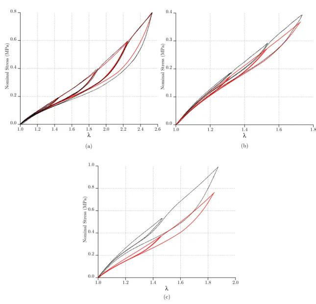
the preconditioning test.

162

These results encourage to consider that the strain energy in the maximal principal

163

strain direction is the governing parameter for the come-back on the first loading curve

164

whatever is the second loading. Moreover, the stress softening amount in the other

di-165

rections are linked to this parameter but it is attenuated if the direction of the maximal

166

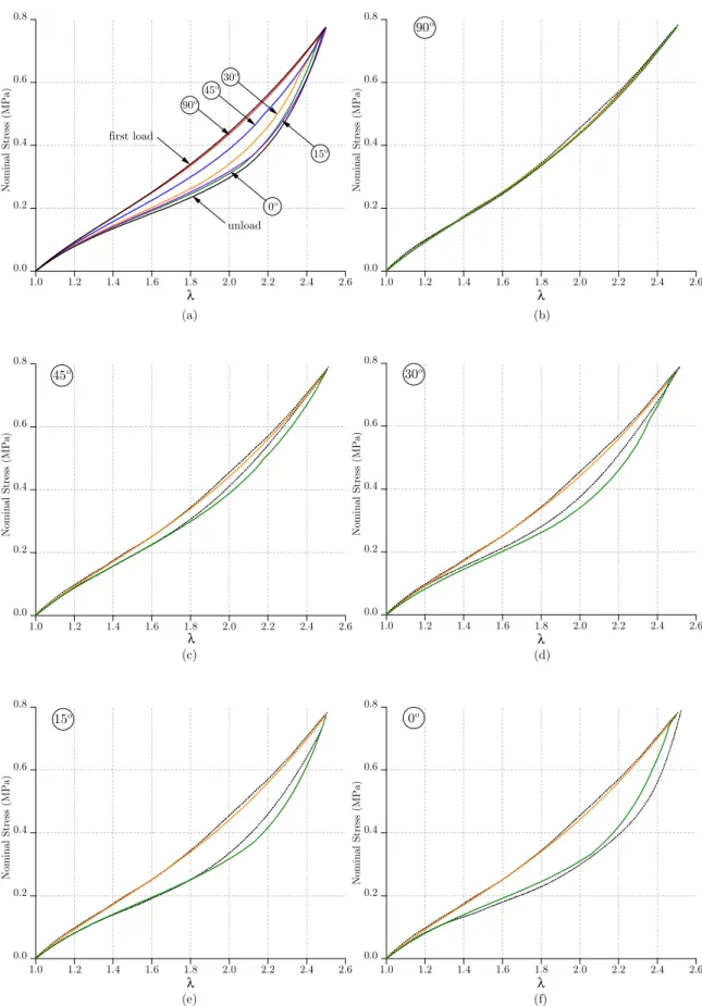
principal strain is not the same between first and second loadings. A measure for these

167

quantities should thus be introduced.

3.2. New measure definition to quantify the stress softening

169

The strain energy is often used to describe the Mullins effect (see references in Machado

170

et al. (2010); Diani et al. (2009)) but its use is limited to the isotropic approach, since

171

energy is a scalar global measure of the deformation state. Therefore, to compare the

172

strain energy in different directions can be the clue. It is thus proposed to introduce a

173

measure of the strain energy given by the contribution of each material direction.

174

Figure 2 illustrates the kinematics of an infinitesimal cone element extracted from the

175

initial spherical representative volume element centered in P of radius dR0. In the initial

176

configuration the slant height, surface area and volume are dR0, dS0 and dV0= 1₃dR0dS0

177

respectively; the unity vector a0 defines the material direction in the undeformed REV.

178

Considering the point Q, lying within an infinitesimal neighborhood of P , defined by the

179

vector dx0 = dR0a0. Under the deformation, this vector is mapped into dx = F dx0,

180

where F is the deformation gradient. Thus, one obtains the following relation

181

dx = F dx0 = dR0Fa0 (2)

In the deformed configuration points p and q are referenced by the position vectors x

182

and x + dx respectively; and the vector normal to the deformed surface dS given by the

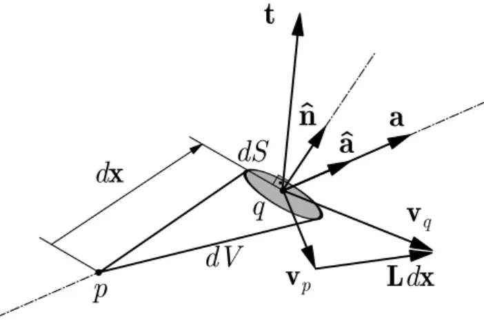
183 Nanson’s relation 184 ˆ n = det(F)dS0 dS F −T_a 0. (3)

The velocity field within the infinitesimal neighborhood of x, with respect the reference

a

a

n

^

a

^

F

Figure 2: Kinematics of an infinitesimal cone element from the spherical REV.

a

n

^

a

^

dx

p

q

dS

v

v

L

_dx

t

dV

Figure 3: Force end velocity vectors in the deformed REV.

frame R is given by

186

vq(x + dx)_/R = vp(x, t)_/R+ L (x, t)_/Rdx (4)

with L (x, t)_/R= W (x, t)_/R+ D (x, t) where L, W and D are the velocity gradient, spin

187

and rate of deformation tensors. In any motion, the velocity field is locally decomposed

188

as a sum of a rigid velocity vp(x, t)/R+ W (x, t)/Rdx and a straining velocity D (x, t) dx.

189

Considering Figure 3, the power P/R = t· (vq)_/R is expended by a force t = σˆn dS 190

acting at point q, where σ is the Cauchy stress tensor. The interest is the expended

191

power associated only with deformations. Then, it is possible to write the strain energy

192

increment dM during a time increment dt, excluding rigid velocity, by the scalar product

193

dM = σˆn dS · Ddx dt (5)

where Ddx is the straining velocity field associated exclusively to the rate of deformation

194

tensor D. Replacing Eq. (3) into Eq. (5), one obtains

195

dM = 3dV0 det(F) [

F−1σDF]: (a0⊗ a0) dt (6)

Finally, the strain energy contribution in the a0 direction is written, per unity of unde-formed volume dV0, as M(a0) = 3 [∫ t 0 det(F) F−1σDF dt ] : (a0⊗ a0) = 3 Ma0· a0 (7)

This permits to introduce a tensor M in Eq. (7), defined in the reference

tion. It is decomposed into a symmetric Msym _{and skew-symmetric M}skew _{part. Note}

197

that the product of a symmetric tensor and a skew-symmetric tensor has zero trace, i.e.,

198

Mskew: (a0⊗ a0) = 0. Thus, in a general formulation, Msym describes the contribution

199

of each material direction in the total strain energy. As symmetric tensor Msympossesses

200

three real eigenvalues (MI > MII > MIII), where the maximal principal value MI is

201

connected with an eigenvector determining the direction of maximum strain energy.

Dif-202

ferent noticeable parameters can be defined. The maximum strain energy for each conical

203

elementary volume in direction a0 along the history is

204

Mmax(a0) = max

τ≤t M(a0, τ ) (8)

At the current time t, the maximum instantaneous strain energy in any direction is defined

205

as

206

I(t) = MI(t) (9)

And last, the maximum strain energy in any direction in the history is defined as

207

G = max

τ≤t MI(t). (10)

3.3. Construction of the evolution equation

208

An evolution function F is introduced along each direction, it describes the evolution

209

of the network in the considered direction. The global strain energy is then rewritten as

210 W = Wcc+ ∫ VREV 0 F(a0)Wcf(a0) dV0. (11)

where V₀REV is the undeformed REV volume. At the sight of the silicone filled rubber

211

experimental data, the functionF(a0) can be written as a function of the characteristic

212

energy measures previously introduced

213

F(a0) =F(M(a0),Mmax(a0),I, G) (12)

The main difference with the models from the literature is that the functionF does not

214

only depend on what happens in the considered direction a0 but also on the global strain

215

energy in the material, i.e.,I and G. Then, different forms can be proposed.

In this paper, the concept for evolution function (Beatty and Krishnaswamy, 2000;

217

Zu˜niga, 2005; Zu˜niga and Rodr´ıguez, 2010) is used. This concept describes the Mullins

218

effect by comparing the current deformation state and the maximum one, that means

219

that the evolution function depends on the difference between the maximum and current

220

deformation state. Thus, the value of introduced function remains one during the first

221

load and it decreases when the current state differs from the maximum state. Thus, during

222

a first loading I = G the function F(a0) should not evolve if the material is stretched in

223

a given direction for the first time, then

224

F(M(a0),Mmax(a0),I = G, G) = 1 (13)

During a second loading curve the function evolves, as the difference between the current

225

and the maximum strain increases, in the interval given by

226

F(M(a0),Mmax(a0),I, G) ∈ [0, 1] (14)

This approach leads to a dependence in (G−I) and (Mmax(a0)−M(a0)) of the constitutive

227

equation. Moreover, the amount of stress softening is directly linked to the orientation

228

of the loading, the ratio of what happens in each direction compared to the maximum

229

deformation should be taken into account. In this way, a general form is proposed as

230 follows 231 F = 1 − F1(G − I) F2(Mmax(a0)− M(a0)) F3 ( Mmax(a0) G ) (15)

whereF1,F2 and F3 are functions to be determined. This multiplicative decomposition,

232

also used in Rebouah et al. (2013), is principally phenomenological, since stress softening

233

is treated as a multiplicative function of the strain energy, see Eq. 11. The conditions

234

evoked in Eq. (13) lead to

235

F1(G − I) = 0 if G = I (16)

F2(Mmax(a0)− M(a0)) = 0 if Mmax(a0)=M(a0). (17)

Now, different constitutive equation forms can be proposed for each function F1, F2 and

236

F3 in Eq. (15).

4. The anisotropic constitutive equation 238

4.1. Hyperelastic constitutive equation

239

The advantage of such formulation is that the first loading curve is independent of the

240

evolution function on the contrary of damage mechanics (Lemaitre and Chaboche, 1990).

241

Thus, the choice of the hyperelastic energy only depends on the first loading curves. In a

242

first approach, it is proposed to use the classical Mooney (1940) constitutive equation to

243

represent the isotropic energy density, then

244

Wcc= C1(I1− 3) + C2(I2− 3) (18)

For the anisotropic part of the constitutive equation the material could be represented

245

by an infinite number of directions, introducing a probability density. But in this study, it

246

is preferred to use a distribution of n−direction a(i)₀ oriented in any direction throughout

247

the three-dimensional space instead of an integral formulation (Eq. 11). Bazant and Oh

248

(1986) proposed different orientation schemes, that define the set of vectors a(i)₀ with

249

different weight ω(i) for each direction to obtain a material as close as possible to an

250

isotropic material when all the chains have the same mechanical behavior. Wcf is then

251 written as 252 Wcf = n ∑ i=1

ω(i)F(i)W_cf(i)(a(i)₀ ) (19)

where n is the number of considered directions and W_cf(i)(a(i)₀ ) is the hyperelastic strain

253

energy of the chain in the initial direction a(i)₀ . The classical centrally symmetric n = 2×21

254

scheme was chosen to represent the material directions. The vector and weight of each

255

direction can be found in Bazant and Oh (1986). All the other direction distribution

256

schemes could also be used. A comparative study of recently proposed integration schemes

257

in application to a full network model of rubber can be found in Ehret et al. (2010).

258

The non-Gaussian theory is classically used to capture the anisotropy. Diani et al.

259

(2006a) and Dargazany and Itskov (2009) use the Langevin chain representation forW_cf(i)

260

energy. The great advantage of this choice is that it brings physical understanding to the

261

modeling and it presents two main consequences. The first is that the zero-stress state is

262

only ensured by the compensation of all the directions contribution as ∂W(λ(i))/∂λ(i)̸= 0

263

material. The second one is that it allows to capture an important permanent

deforma-265

tion of the material after a loading cycle. However, in filled silicone experiments, it was

266

shown that the permanent deformation is quite negligible. To this purpose, the

classi-267

cal hyperelastic anisotropic approach using the strain invariant I₄(i) = a(i)T₀ C a(i)₀ is used,

268

where C = FTF is the right Cauchy-Green strain tensor. The function should verify the 269 following conditions 270 W(i) cf(I (i) 4 ) = 0 if I (i) 4 = 1 (20) ∂W(i) cf(I (i) 4 ) ∂I₄(i) = 0 if I (i) 4 = 1. (21)

In a first approach, an ordinary constitutive equation is used, considering that the chains

271

are only stretched by tensile stresses. Otherwise, it is considered that compressive stretches

272

lead to buckling. Thus, one may write

273 W(i) cf = K(i) 2 ( I₄(i)− 1 )2 if I₄(i) ≥ 1 else 0. (22)

This formulation can be adapted to non-initially isotropic materials by choosing different

274

functions forW_cf(i). As the filled silicone rubber is initially isotropic, everyW_cf(i) is initially

275

the same in all directions, i.e.,∀i, j K(i)= K(j).

276

4.2. stress softening constitutive equation

277

In part 3.3, a multiplicative decomposition was postulated in Eq. (15). The use of

278

simple power functions, for F1, F2 and F3, is proposed to represent the stress softening,

279 given by 280 F(i) _{= 1− η} √ G − I G √ M(i) max− M(i) G ( M(i) max G )2 (23)

where η is a material parameter. The functions F1 and F2 are normalized according to

281

the maximum strain energy G to ensure a normalized evolution function for each second

282

loading curve. It is important to note that, even if the objective is to describe Mullins effect

283

anisotropy, the constitutive equation for stress softening only depends on one parameter η.

284

All the other parameters describe the hyperelastic first loading. The evolution functions

285

have the same form in all directions, but this approach could be extended to non-isotropic

286

stress softening function by defining different values for the parameter η in the different

directions.

288

There remains to verify that the presented model is in agreement with the requirements

289

of thermodynamics (see e.g. Coleman and Gurtin, 1967). If only isothermal processes is

290

considered, the Clausius-Duhem inequality must be satisfied by the conditions

291 − ∂W ∂M(i)max ˙ M(i) max> 0 (24) −∂W ∂G G > 0˙ (25)

where ˙M(i)max> 0 and ˙G > 0. By means of straightforward manipulations of Eqs. (11), (24)

292

and (25) one can easily establish the above relations in terms of the evolution function

293

F(i)_{. It is also important to show that}

294 ∂F(i) ∂M(i)max 6 0, ∀i (26) ∂F(i) ∂G 6 0, ∀i. (27)

Considering the form of Eq. (23), the explicit form for Eq. (26) is given by

295 −η √ G − I G 1 G  1 2 ( M(i) max−M G )₋1 2 ( M(i) max G )2 + 2 ( M(i) max G ) √ M(i) max−M G   6 0, ∀i.(28) First, an elementary study of the Eq.(28) shows that all fractions terms are positive.

296

Second, when the stress softening evolves, i.e.,G increasing, the maximum instantaneous

297

strain energy I is equal to the maximum G. Thus, the function remains equal zero and

298

the condition of Eq. (26) is automatically satisfied. In this way, the choice of F respects

299

the conditions of Eqs.(26) and (27) and consequently the Clausius-Duhem inequality is

300

satisfied.

301

4.3. Comparison of the modeling with experimental data

302

The model is fitted on all the experimental data presented in Machado et al. (2010,

303

2012a), i.e., tests where the principal stretch directions remain unchanged during first

304

and second load or tests where the principal stretch directions are not necessarily the

305

same during first and second loads. First, the parameters of the hyperelastic constitutive

306

equations are fitted on the different first loading curves. Different parameters can be

307

chosen according to the repartition of the strain energy betweenWcc and Wcf.

Considering a second tensile loading immediately before the sample rupture, the most

309

stress softening level is obtained and this state corresponds to the strain energy of chains

310

that were not affected by the Mullins effect. Thus, to ensure a good balance betweenWcc

311

andWcf the portionWcc, i.e., the Mooney model, is fitted on the beginning of the second

312

tensile loading curve at the higher deformation achieved before rupture.

313

Next, the part ofWcf is fitted to complete the stress amount of the first loading curves.

314

The fitted parameters are presented in Table 1.

315

Table 1: Values of the constitutive equation parameters

Parameter Value

C1 0.05 MPa

C2 0.03 MPa

∀i K(i) _{0.20 MPa}

η 1.0

The last parameter that describes the stress softening is fitted on the second loading

316

curves for all the tests, the value η = 1.0 is obtained. The condition in Eq. (14) must be

317

satisfied, and as explained the function F(i) cannot be negative. If its softening is too

318

large, i.e., F(i) < 0, the value F(i) = 0 is imposed. That means that in the considered

319

direction a great number of chain–filler links were broken. In the second load, for the

320

same direction, the suspended chains are no longer acting enough to impose a force on

321

the macromolecular network, i.e., they do not contribute to the network entropic energy

322

any more and their energy is thus lost (Dargazany and Itskov, 2009). This assumption

323

is consistent with the two networks theory and justified for relative short chains. Note

324

that for longer molecular chains bonded at different places to fillers this assumption can

325

be relaxed, for example, to take into account permanent set.

326

The simulations of the cyclic uniaxial tensile, pure shear and equibiaxial tensile tests

327

are presented in Fig. 4. Concerning the first load, it appears that the model describes

328

adequately uniaxial and pure shear tests whereas equibiaxial tests are underestimated.

329

This phenomenon is due to the hyperelastic equation and not to stress softening equation.

330

As pointed out by Marckmann and Verron (2006) and Boyce and Arruda (2000), there

331

are very few hyperelastic constitutive models able to simultaneously simulate the both

332

multi-dimensional data with a unique set of material parameters. Concerning the cyclic

333

behavior, the form of the stress softening for all tests is quite well described. For uniaxial

tensile and pure shear curves, the model has a slight tendency to underestimate stress

335

softening and it is even more pronounced for equibiaxial tensile test.

336

Figure 4: Comparison of the model (solid lines) with experimental data from Machado et al. (2010) (dotted lines) for: (a) cyclic uniaxial tensile test, (b) cyclic pure shear test and (c) cyclic equibiaxial test.

Next, tensile tests with a change of loading direction between the first and second

337

loads are confronted. A simulation of the modeling is presented in Fig. 5(a). It appears

338

that the trend of simulations are exactly what experimentally happens. All the second

339

loading curves come back on the same point of the first loading curve and the amount of

340

stress softening is directly linked to the angle between the principal stretch directions of

341

the first and second loads. A detailed comparison with experimental data is presented in

342

Fig. 5(b-f). The model does not superpose perfectly all experimental data, but all trends

343

are quite well described.

Figure 5: Comparison of the model (solid lines) with TT uniaxial prestretching experimental data (dotted lines). (a) simulation of the model for different orientations of the second load. Details of the experimental (dotted lines) and modeled (solid lines) first and second load curves with an angle between stretch direction of: (b) 90◦, (c) 45◦, (d) 30◦, (e) 15◦and (f) 0◦.

To finish, the model is used to simulate BT tests, the first load being a biaxial test

345

and the second load being a tensile test. The comparison of the second loading curves is

346

presented in Fig. 6. It appears that stress softening is moderately overestimated by the

347

model, however the come-back on the first loading curve is perfectly described.

348

Figure 6: Comparison of the model (solid lines) with BT biaxial prestretching experimental data (dotted lines). Curve a: simulation of the model for the second tensile load after an equibiaxial test; curve g: simulation of the model for the second load after a biaxial test of biaxiality ratio µ = 0.7; curve h: simulation of the model for the second load after a biaxial test of biaxiality ratio µ = 0.5

All these simulations emphasize that the use of this new elongation energy measure is

349

a good point to describe the come back of the second loading curves on the virgin one.

350

The amount of stress softening is well described for cyclic loading experiments and for

351

TT tests, where the principal stretch directions were not the same during first and second

352

loads. Nevertheless, the stress softening during BT test is overestimated. As observed

353

in Fig. 4(c), stress was underestimated for the equibiaxial state, but this is due to the

354

underestimation of hyperelastic strain energy obtained at the first load.

355

It can be noticed that the model describes correctly all the experimental tests with a

356

simple constitutive equation that only depends on one parameter. Evidently, the results

357

can be improved by proposing more complex constitutive equations, that consequently

358

would lead to a significant increase in the number of parameters. Nevertheless, the

pre-359

sented results allowed to demonstrate the efficiency of this new approach.

5. Conclusion 361

This paper presents an original approach to model the stress induced anisotropy by the

362

Mullins effect, by the definition of a tensor to measure the repartition of the strain energy

363

in space. The comparison of the strain energy in different directions with the maximal

364

principal strain energy permits to create a new formulation for stress softening modeling.

365

In this approach, the constitutive equation is written in function of the variation of strain

366

energy in each direction and the variation of strain energy in the maximal principal strain

367

direction. This new approach captures the principal characteristics of the Mullins effect

368

underlined in literature. This new way of describing Mullins effect anisotropy can be a

369

good starting point to elaborate new constitutive equations.

370

In this paper, a simple constitutive equation to describe the stress softening evolution

371

was proposed. It clearly appears that the results are quite encouraging for a model that

372

can describe many different types experimental tests, with very different strain histories,

373

and the models presents only one material parameter. Of course, the agreement with

374

the experimental data can be improved by using more sophisticated constitutive equation

375

forms.

376

6. Acknowledge 377

We would like to thank the French ANR for supporting this work through the project

378

RAAMO (”Robot Anguille Autonome pour Milieux Opaques”)

379

References 380

Arruda, E. M. and Boyce, M. C. (1993). A three dimensional constitutive model for the large stretch

381

behavior of rubber elastic materials. J. Mech. Phys. Solids, 41(2), 389–412.

382

Bazant, Z. P. and Oh, B. H. (1986). Efficient numerical integration on the surface of a sphere. Z. Angew.

383

Math. Mech., 66, 37–49.

384

Beatty, M. F. and Krishnaswamy, S. (2000). A theory of stress-softening in incompressible isotropic

385

materials. J. Mech. Phys. Solids, 48, 1931–1965.

386

Besdo, D., Ihlemann, J., Kingston, J., and Muhr, A. (2003). Modelling inelastic stress-strain phenomena

387

and a scheme for efficient experimental characterization. In: Busfield, Muhr (eds) Constitutive models

388

for Rubber III. Swets & Zeitlinger, Lisse., pages 309–317.

389

Boyce, M. C. and Arruda, E. M. (2000). Constitutive models of rubber elasticity: A review. Rubber Chem.

390

Technol., 73, 504–523.

Chagnon, G., Verron, E., Gornet, L., Marckmann, G., and Charrier, P. (2004). On the relevance of

392

Continuum Damage Mechanics as applied to the Mullins effect in elastomers. J. Mech. Phys. Solids,

393

52, 1627–1650. 394

Coleman, B. D. and Gurtin, M. E. (1967). Thermodynamics with internal state variables. J. Chem. Phys.,

395

47(2), 597–613. 396

Dargazany, R. and Itskov, M. (2009). A network evolution model for the anisotropic Mullins effect in

397

carbon black filled rubbers. Inter. J. Solids Struct., 46(16), 2967 – 2977.

398

Diani, J., Brieu, M., and Vacherand, J. M. (2006a). A damage directional constitutive model for the

399

Mullins effect with permanent set and induced anisotropy. Eur. J. Mech. A/Solids, 25, 483–496.

400

Diani, J., Brieu, M., and Gilormini, P. (2006b). Observation and modeling of the anisotropic

visco-401

hyperelastic behavior of a rubberlike material. Int. J. Solids Struct., 43, 3044–3056.

402

Diani, J., Fayolle, B., and Gilormini, P. (2009). A review on the Mullins effect. Eur. Polym. Journal, 45,

403

601–612.

404

Dorfmann, A. and Ogden, R. W. (2003). A pseudo-elastic model for loading, partial unloading and

405

reloading of particle-reinforced rubbers. Int. J. Solids Struct., 40, 2699–2714.

406

Dorfmann, A. and Pancheri, F. (2012). A constitutive model for the Mullins effect with changes in material

407

symmetry. International Journal of Non-Linear Mechanics, 47(8), 874 – 887.

408

Ehret, A. E., Itskov, M., and Schmid, H. (2010). Numerical integration on the sphere and its effect on the

409

material symmetry of constitutive equations - A comparative study. Int. J. Numer. Meth. Eng., 81(2),

410

189–206.

411

G¨oktepe, S. and Miehe, C. (2005). A macro approach to rubber-like materials. Part III: The

micro-412

sphere model of anisotropic Mullins-type damage. J. Mech. Phys. Solids, 53, 2259–2283.

413

Govindjee, S. and Simo, J. C. (1991). A micro-mechanically continuum damage model for carbon black

414

filled rubbers incorporating Mullins’s effect. J. Mech. Phys. Solids, 39(1), 87–112.

415

Govindjee, S. and Simo, J. C. (1992). Transition from micro-mechanics to computationally efficient

phe-416

nomenology: Carbon black-filled rubbers incorporating Mullins’s effect. J. Mech. Phys. Solids, 40(1),

417

213–233.

418

Green, M. S. and Tobolsky, A. V. (1946). A new approach for the theory of relaxing polymeric media. J.

419

Chem. Phys., 14, 87–112.

420

Hanson, D. E., Hawley, M., Houlton, R., Chitanvis, K., Rae, P., Orler, E. B., and Wrobleski, D. A. (2005).

421

Stress softening experiments in silica-filled polydimethylsiloxane provide insight into a mechanism for

422

the Mullins effect. Polymer, 46(24), 10989 – 10995.

423

Itskov, M., Ehret, A., Kazakeviciute-Makovska, R., and Weinhold, G. (2010). A thermodynamically

424

consistent phenomenological model of the anisotropic Mullins effect. J. Appl. Math. Mech., 90(5),

425

370–386.

426

Lemaitre, J. and Chaboche, J. L. (1990). Mechanics of solid materials. Cambridge University Press.

427

Li, J., Mayau, D., and Lagarrigue, V. (2008). A constitutive model dealing with damage due to cavity

428

growth and the Mullins effect in rubber-like materials under triaxial loading. J. Mech. Phys. Solids,

429

56(3), 953 – 973. 430

Machado, G., Chagnon, G., and Favier, D. (2010). Analysis of the isotropic models of the Mullins effect

431

based on filled silicone rubber experimental results. Mech. Mater., 42(9), 841 – 851.

432

Machado, G., Chagnon, G., and Favier, D. (2012a). Induced anisotropy by the Mullins effect in filled

433

silicone rubber. Mech. Mater., 50, 70 – 80.

434

Machado, G., Favier, D., and Chagnon, G. (2012b). Membrane curvatures and stress-strain full fields of

ax-435

isymmetric bulge tests from 3D-DIC measurements. Theory and validation on virtual and experimental

436

results. Exp. Mech., 52, 865–880.

437

Marckmann, G. and Verron, E. (2006). Comparison of hyperelastic models for rubber-like materials. Rubber

438

Chem. Technol., 79(5), 835–858.

439

Marckmann, G., Verron, E., Gornet, L., Chagnon, G., and Fort, P. C. P. (2002). A theory of network

440

alteration for the Mullins effect. J. Mech. Phys. Solids., 50, 2011–2028.

441

Merckel, Y., Diani, J., Roux, S., and Brieu, M. (2011). A simple framework for full-network hyperelasticity

442

and anisotropic damage. J. Mech. Phys. Solids., 59(1), 75 – 88.

443

Merckel, Y., Brieu, M., Diani, J., and Caillard, J. (2012). A Mullins softening criterion for general loading

444

conditions. J. Mech. Phys. Solids., 60(7), 1257 – 1264.

445

Miehe, C. (1995). Discontinuous and continuous damage evolution in Ogden type large strain elastic

446

materials. Eur. J. Mech., A/Solids, 14(5), 697–720.

447

Mooney, M. (1940). A theory of large elastic deformation. J. Appl. Phys., 11, 582–592.

448

Muhr, A. H., Gough, J., and Gregory, I. H. (1999). Experimental determination of model for liquid

449

silicone rubber: Hyperelasticity and Mullins effect. In Proceedings of the First European Conference on

450

Constitutive Models for Rubber, pages 181–187. Dorfmann A. Muhr A.

451

Mullins, L. (1947). Effect of stretching on the properties of rubber. J. Rubber Res., 16, 275–289.

452

Ogden, R. W. and Roxburgh, D. G. (1999). A pseudo-elastic model for the Mullins effect in filled rubber.

453

Proc. R. Soc. Lond. A, 455, 2861–2877.

454

Rebouah, M., Machado, G., Chagnon, G., and Favier, D. (2013). Anisotropic mullins stress softening of a

455

deformed silicone holey plate. Mechanics Research Communications, 49(0), 36 – 43.

456

Rey, T., Chagnon, G., Le Cam, J.-B., Favier, D.(2013). Influence of the temperature on the mechanical

457

behaviour of filled and unfilled silicone rubbers. Polym. Test., 32, 492–501.

458

Shariff, M. H. B. M. (2006). An anisotropic model of the Mullins effect. J. Eng. Math., 56(4), 415–435.

459

Simo, J. C. (1987). On a fully three-dimensional finite-strain viscoelastic damage model: formulation and

460

computational aspects. Comp. Meth. Appl. Mech. Engng, 60, 153–173.

461

Z´u˜niga, A. E. and Beatty, M. F. (2002). A new phenomenological model for stress-softening in elastomers.

462

Z. Angew. Math. Phys., 53, 794–814.

463

Z´u˜niga, A. E. (2005). A phenomenological energy-based model to characterize stress-softening effect in

464

elastomers. Polymer, 46, 3496–3506.

465

Z´u˜niga, A. E. and Rodr´ıguez, C. (2010). A non-monotonous damage function to characterize

stress-466

softening effects with permanent set during inflation and deflation of rubber balloons. Int. J. Eng. Sci.,

467

48(12), 1937 – 1943. 468