HAL Id: hal-01300334
https://hal.archives-ouvertes.fr/hal-01300334
Submitted on 10 Apr 2016
HAL is a multi-disciplinary open access
archive for the deposit and dissemination of
sci-entific research documents, whether they are
pub-lished or not. The documents may come from
L’archive ouverte pluridisciplinaire HAL, est
destinée au dépôt et à la diffusion de documents
scientifiques de niveau recherche, publiés ou non,
émanant des établissements d’enseignement et de
Solving the Team Orienteering Problem with Cutting
Planes
Racha El-Hajj, Duc-Cuong Dang, Aziz Moukrim
To cite this version:
Racha El-Hajj, Duc-Cuong Dang, Aziz Moukrim.
Solving the Team Orienteering Problem
with Cutting Planes.
Computers and Operations Research, Elsevier, 2016, 74, pp.21-30.
�10.1016/j.cor.2016.04.008�. �hal-01300334�
Solving the Team Orienteering Problem
with Cutting Planes
Racha El-Hajja,c,∗, Duc-Cuong Dangb, Aziz Moukrima
a
Sorbonne universit´es, Universit´e de technologie de Compi`egne CNRS, Heudiasyc UMR 7253, CS 60 319, 60 203 Compi`egne cedex
b
University of Nottingham, School of Computer Science Jubilee Campus, Wollaton Road, Nottingham NG8 1BB, United Kingdom
c
Universit´e Libanaise, ´Ecole Doctorale des Sciences et de Technologie Campus Hadath, Beyrouth, Liban
Abstract
The Team Orienteering Problem (TOP) is an attractive variant of the Vehicle Routing Problem (VRP). The aim is to select customers and at the same time organize the visits for a vehicle fleet so as to maximize the collected profits and subject to a travel time restriction on each vehicle. In this paper, we investigate the effective use of a linear formulation with polynomial number of variables to solve TOP. Cutting planes are the core components of our solving algorithm. It is first used to solve smaller and intermediate models of the original problem by considering fewer vehicles. Useful information are then retrieved to solve larger models, and eventually reaching the original problem. Relatively new and dedi-cated methods for TOP, such as identification of irrelevant arcs and mandatory customers, clique and independent-set cuts based on the incompatibilities, and profit/customer restriction on subsets of vehicles, are introduced. We evaluated our algorithm on the standard benchmark of TOP. The results show that the algorithm is competitive and is able to prove the optimality for 12 instances previously unsolved.
Keywords: Team Orienteering Problem, cutting planes, dominance property, incompatibility, clique cut, independent-set cut.
1. Introduction
The Team Orienteering Problem (TOP) was first mentioned in Butt and Cavalier (1994) as the Multiple Tour Maximum Collection Problem (MTMCP). Later, the term TOP was formally introduced in Chao et al. (1996). TOP is a
∗corresponding author
Email addresses: [email protected](Racha El-Hajj ),
[email protected](Duc-Cuong Dang), [email protected] (Aziz Moukrim)
variant of the Vehicle Routing Problem (VRP) (Archetti et al. 2014). In this variant, a limited number of identical vehicles is available to visit customers from a potential set. Two particular depots, the departure and the arrival points are considered. Each vehicle must perform its route starting from the departure depot and returning to the arrival depot without exceeding its predefined travel time limit. A certain amount of profit is associated for each customer and must be collected at most once by the fleet of vehicles. The aim of solving TOP is to organize an itinerary of visits respecting the above constraints for the fleet in such a way that the total amount of collected profits from the visited customers is maximized.
A special case of TOP is the one with a single vehicle. The resulted problem is known as the Orienteering Problem (OP), or the Selective Travelling Salesman Problem (STSP) (see the surveys by Feillet et al. 2005, Vansteenwegen et al. 2011 and Gavalas et al. 2014). OP/STSP is already NP-Hard (Laporte and Martello 1990), and so is TOP (Chao et al. 1996). The applications of TOP arise in various situations. For example in Bouly et al. (2008), the authors used TOP to model the schedule of inspecting and repairing tasks in water distribution. Each task in this case has a specific level of urgency which is similar to a profit. Due to the limitation of available human and material resources, the efficient selection of tasks as well as the route planning become crucial to the quality of the schedule. A very similar application was described in Tang and Miller-Hooks (2005) to route technicians to repair sites. In Souffriau et al. (2008), Vansteenwegen et al. (2009) and Gavalas et al. (2014), the tourist guide service that offers to the customers the possibility to personalize their trips is discussed as variants of TOP/OP. In this case, the objective is to maximize the interest of customers on attractive places subject to their duration of stay. Those planning problems are called Tourist Trip Design Problems (TTDPs). Many other applications include the team-orienteering sport game, bearing the original name of TOP, the home fuel delivery problem with multiple vehicles (e.g., Chao et al. 1996) and the athlete recruiting from high schools for a college team (e.g., Butt and Cavalier 1994).
Many heuristics have been proposed to solve TOP, like the ones in Archetti et al. (2007), Souffriau et al. (2010), Dang et al. (2013b) and Kim et al. (2013). These approaches are able to construct solutions of good quality in short com-putational times, but those solutions are not necessarily optimal. In order to validate them and evaluate the performance of the heuristic approaches, either optimal solutions or upper bounds are required. For this reason, some researches have been dedicated to elaborate exact solution methods for TOP. Butt and Ryan (1999) introduced a procedure based on the set covering formulation. A column generation algorithm was developed to solve this problem. In Boussier et al. (2007), the authors proposed a branch-and-price (B-P) algorithm in which they used a dynamic programming approach to solve the pricing problem. Their approach has the advantage of being easily adaptable to different variants of the problem. Later, Poggi de Arag˜ao et al. (2010) introduced a pseudo-polynomial linear model for TOP and proposed a branch-cut-and-price (B-C-P) algorithm. New classes of inequalities, including min-cut and triangle clique, were added to
the model and the resulting formulation was solved using a column generation approach. Afterwards, Dang et al. (2013a) proposed a branch-and-cut (B-C) al-gorithm based on a linear formulation and features a new set of valid inequalities and dominance properties in order to accelerate the solution process. Recently, Keshtkarana et al. (2016) proposed a Branch-and-Price algorithm with two re-laxation stages (B-P-2R) and a Branch-and-Cut-and-Price (B-C-P) approach to solve TOP, where a bounded bidirectional dynamic programming algorithm with decremental state space relaxation was used to solve the subproblems. These five methods were able to prove the optimality for a large part of the standard benchmark of TOP (Chao et al. 1996), however there is a large num-ber of instances that are still open until now. Furthermore, according to the recent studies of Dang et al. (2013b) and Kim et al. (2013), it appears that it is hardly possible to improve the already-known solutions for the standard bench-mark of TOP using heuristics. These studies suggest that the known heuristic solutions could be optimal but there is a lack of variety of effective methods to prove their optimality.
Motivated by the above facts, in this paper we propose a new exact algorithm to solve TOP. It is based on a linear formulation with a polynomial number of binary variables. Our algorithmic scheme is a cutting plane algorithm which exploits integer solutions of successive models with the subtour elimination con-straints being relaxed at first and then iteratively reinforced. Recently, Pferschy and Stanˇek (2013) demonstrates on the Travelling Salesman Problem (TSP) that such a technique which was almost forgotten could be made efficient nowaday with the impressive performance of modern solvers for Mixed-Integer Program-ming (MIP), especially with a careful control over the reinforcing of the subtour elimination. Our approach is similar but in addition to subtour elimination, we also make use of other valid inequalities and useful dominance properties to enhance the intermediate models. The properties include breaking the sym-metry and exploiting bounds or optimal solutions of smaller instances/models with fewer number of vehicles, while the proposed valid inequalities are the clique cuts and the independent set cuts based on the incompatibilities between customers and between arcs. In addition, bounds on smaller restricted models are used to locate mandatory customers and inaccessible customers/arcs. Some of these cuts were introduced and tested in Dang et al. (2013a) yielding some interesting results for TOP, this encourages us to implement them immediately in our cutting plane algorithm. We evaluated our algorithm on the standard benchmark of TOP. The obtained results clearly show the competitiveness of our algorithm. The algorithm is able to prove the optimality for 12 instances that none of the previous exact algorithms had been able to solve.
The remainder of the paper is organized as follows. A short description of the problem with its mathematical formulation is first given in Section 2, where the use of the generalized subtour elimination constraints is also discussed. In Section 3, the set of dominance properties, which includes symmetry breaking, removal of irrelevant components, identification of mandatory customers and boundaries on profits/numbers of customers, is presented. The graphs of in-compatibilities between variables are also described in this section, along with
the clique cuts and the independent set cuts. In Section 4, all the techniques used to generate these efficient cuts are detailed, and the pseudocode of the main algorithmic scheme is given. Finally, the numerical results are discussed in Section 5, and some conclusions are drawn.
2. Problem formulation
TOP is modeled with a complete directed graph G = (V, A) where V = {1, . . . , n} ∪ {d, a} is the set of vertices representing the customers and the depots, and A = {(i, j) | i, j ∈ V, i 6= j} the set of arcs linking the different vertices together. The departure and the arrival depots for the vehicles are represented by the vertices d and a. For convenience, we use the three sets V−, Vd and Va to denote respectively the sets of the customers only, of the
customers with the departure depot and of the customers with the arrival one. A profit pi is associated for each vertex i and is considered zero for the two
depots (pd = pa = 0). Each arc (i, j) ∈ A is associated with a travel cost cij.
Theses costs are assumed to be symmetric and to satisfy the triangle inequality. All arcs incoming to the departure depot and outgoing from the arrival one must not be considered (cid = cai= ∞, ∀i ∈ V−). Let F represent the fleet of
the m identical vehicles available to visit customers. Each vehicle must start its route from d, visit a certain number of customers and return to a without exceeding its predefined travel cost limit L. Using these definitions, we can formulate TOP with a linear Mixed Integer Program (MIP) using a polynomial number of decision variables yirand xijr. Variable yiris set to 1 if vehicle r has
served client i and to 0 otherwise, while variable xijr takes the value 1 when
vehicle r uses arc (i, j) to serve customer j immediately after customer i and 0 otherwise. max X i∈V− X r∈F yirpi (1) X r∈F yir≤ 1 ∀i ∈ V− (2) X j∈Va xdjr = X j∈Vd xjar = 1 ∀r ∈ F (3) X i∈Va\{k} xkir= X j∈Vd\{k} xjkr = ykr ∀k ∈ V−, ∀r ∈ F (4) X i∈Vd X j∈Va\{i} cijxijr ≤ L ∀r ∈ F (5) X (i,j)∈U×U xijr≤ |U | − 1 ∀U ⊆ V−, |U | ≥ 2, ∀r ∈ F (6) xijr∈ {0, 1} ∀i ∈ V, ∀j ∈ V, ∀r ∈ F (7) yir∈ {0, 1} ∀i ∈ V−, ∀r ∈ F
The objective function (1) maximizes the sum of collected profits from the visited customers. Constraints (2) impose that each customer must be visited at most once by one vehicle. Constraints (3) guarantee that each vehicle starts its path at vertex d and ends it at vertex a, while constraints (4) ensure the connectivity of each tour. Constraints (5) are used to impose the travel length restriction, while constraints (6) eliminate all possible subtours, i.e. cycles ex-cluding the depots, from the solution. Finally, constraints (7) set the integral requirement on the variables.
Enumerating all constraints (6) yields a formulation with an exponential number of constraints. In practice, these constraints are first relaxed from the formulation, then only added to the model whenever needed. The latter can be detected with the presence of subtours in the solution of the relaxed model. We also replace constraints (6) with the stronger ones, the so-called Generalized Subtour Elimination Constraints (GSECs) which enhance both the elimination of specific subtours and the connectivity in the solution. The first GSEC experiment with OP were reported in Fischetti et al. (1998).
We adapted the GSEC version from Dang et al. (2013a) formulated to TOP with a directed graph as follows. For a given subset S of customer vertices, we define δ(S) to be the set of arcs that connect vertices in S with those outside S, i.e. vertices in V \S. We also use γ(S) to represent the set of arcs interconnecting vertices in S. The following GSECs are then added to the model to ensure that each customer served by vehicle r belongs to a path that is connected to the depots and does not form a cycle with other vertices of S.
X
(u,v)∈δ(S)
xuvr≥ 2yir, ∀S ⊂ V, {d, a} ⊆ S, ∀i ∈ V \ S, ∀r ∈ F (8)
We also add two categories of constraints, which are detailed below and are equivalent to the GSECs, to strengthen the model.
X (u,v)∈γ(S) xuvr≤ X i∈S\{d,a} yir− yjr+ 1, ∀S ⊂ V, {d, a} ⊆ S, ∀j ∈ V \ S, ∀r ∈ F (9) X (u,v)∈γ(U) xuvr≤ X i∈U yir− yjr, ∀U ⊆ V−, ∀j ∈ U, ∀r ∈ F (10)
On the other hand, our approach requires a check on the absence of subtours for an optimal solution of the current incomplete model (i.e. while relaxing constraints (6)), so that the global optimality can be claimed. In our model, each strong connected component of the subgraph associated with a tour of the solution represents a subtour, thus the checking can be done by examining the corresponding subgraphs. This will be detailed in Section 4.1.
3. Efficient cuts
Reduction of the search space is often desired in solving a MIP. This can be done by either removing irrelevant components from the linear formulation, e.g.
those that certainly does not belong to any optimal solution, or by favoring some special structures inside the optimal solutions, e.g. reduction of the symmetry. The cuts that we added to our basic problem include some dominance prop-erties as symmetry breaking inequalities, boundaries on profits and number of served customers, cuts that enforces mandatory customers and cuts that remove inaccessible customers and arcs. Moreover, some additional cuts are based on the clique and the independent sets deduced from the incompatibilities between solution components.
3.1. Symmetry breaking cuts
Tours of the optimal solutions can be sorted according to a specific criterion, i.e. the amount of collected profits, the number of customers or the tour length. Based on the experimental report in (Dang et al. 2013a), we focus exclusively on solutions in which the profits of tours are in ascending order. The following constraints are added to the model to ensure the symmetric breaking on profits.
X i∈V− yi(r+1)pi− X i∈V− yirpi≤ 0, ∀r ∈ F \ {m} (11)
Without these constraints, for each feasible solution having different prof-its among prof-its tours, there are at least (m! − 1) equivalently feasible solutions. Adding these constraints will remove these equivalent solutions from the search space and only retain the one having the profits of its tours in ascending order. Thus the size of the search space can be largely reduced.
3.2. Irrelevant components cuts
One simple way of reducing the size of the problem is to deal only with accessible customers and arcs. A customer is considered as inaccessible if by serving only that customer, the travel cost of the resulting tour exceeds the cost limit L. In a similar way, we detect an inaccessible arc when the length of the tour directly connecting the depots to that arc exceeds L. To make a proper linear formulation, all inaccessible customers and arcs are eliminated at the beginning from the model by adding the following constraints. Here i is an inaccessible customer (resp. (i, j) is an inaccessible arc).
X r∈F yir= 0 (12) X r∈F xijr= 0 (13)
3.3. Boundaries on profits and numbers of customers served
Dang et al. (2013a) proposed in their paper a set of efficient dominance properties that aims to reduce the search space by bounding the characteristics of each tour or subset of tours. The idea is to solve within a limited time budget, instances derived from the original problem to gain useful information for the
construction of the added cuts. The derived instances are often smaller than the original one and hopefully easier to solve, or at least to bound.
Before going in the details of these properties, we must clarify some notation. For each instance X with m vehicles, define XI to be the modified instance for
which the profits of each customer is set to 1 instead. We also use Xg to
denote the modified instance X by reducing the number of available vehicles to g (g ≤ m). For g = m, we have the original instance X. Note that the two modifications can be applied at the same time, in this case instance XIg is obtained. Finally, we denote by LB(X) (resp. UB(X)) a lower (resp. an upper) bound of an arbitrary instance X. The following valid inequalities are added to the model to restrict the profits that each tour or subset of tours can have.
X r∈H X i∈V− yirpi≤ UB(X|H|), ∀H ⊂ F (14) X r∈H X i∈V− yirpi+ UB(Xm−|H|) ≥ LB(X), ∀H ⊆ F (15)
Inequalities (14) are trivial since the sum of profits of any |H| tours on the left-hand side cannot exceed the optimal profit of the instance with exactly |H| vehicles or at least an upper bound of this instance, i.e. the right-hand side.
Inequalities (15) work in the opposite direction by applying a lower bound to the profit of each tour and each subset of tours. The inequalities might appear to be redundant with the objective of optimization. However when applied to subsets of tours, the constraints will eliminate unbalanced solutions, e.g. the one with one tour having many customers and the other tours being almost empty, from the search space.
In the same fashion as (14), the numbers of customers per tour or per subset of tours are bounded from above using inequalities (16). On the other hand, it is more difficult to bound these numbers from below since their values do not necessarily correlate with the objective value of TOP. A modification of the model (rather than a simple modification of the instance) is performed in order to determine a lower bound for the number of customers of each tour. This modification is done as follows. We consider the modified instance, denoted by
¯ X1
I, where the objective function is reversed to minimization, i.e. minimizing the
number of served customers, while satisfying both constraints (14) and (15) for |H| = 1. Solving this instance provides the value of LB( ¯X1
I), which enables us
to lower bound the number of customers of each tour of X. The following valid inequalities are then added to the model to restrict the number of customers served in each tour or subset of tours.
X r∈H X i∈V− yir≤ UB(XI|H|), ∀H ⊂ F (16) X i∈V− yir≥ LB( ¯XI1), ∀r ∈ F (17)
In implementation, inequalities (14) - (17) are applied similarly to dynamic programming, as follows. The required values of LB and UB are first computed for the instance with |H| = 1 , then the obtained values are used in the cuts to solve the other instances (|H| ≤ m). We recall that inequalities (17) are limited to a single tour and not subsets of tours. Since the value of UB(Xm−1)
is needed for the model of ¯X1
I, LB( ¯XI1) can only be computed after solving all
the other subproblems (or derived instances). 3.4. Mandatory customers cuts
Given an instance X of TOP, a high quality LB(X) can often be computed efficiently with heuristics. Therefore, it could be possible to locate a set of customers of X, the so-called mandatory ones, for which without one of those customers a solution with the objective value at least as large as LB(X) cannot be achieved.
The formal definition is the following. Here we use X \ {i} to designate the modified instance X with customer i removed.
Definition 1. A customer i of X is mandatory if UB(X \ {i}) < LB(X). Once identified, mandatory customers have to be all served in an optimal solution. The following cuts can then be added to enforce the presence of a mandatory customer i in X.
X
r∈F
yir= 1 (18)
3.5. Valid inequalities based on incompatibilities
If two given customers are too far away from each other because of the travel length/cost limitation, then it is unlikely that they can be served by the same vehicle. This observation leads us to the concept of incompatibility between customers, from which additional inequalities can be deduced (Manerba and Mansini 2015, Gendreau et al. 2016). Moreover, the idea can also be generalized to other pairs of components of the problem, i.e. customer-tour, customer-arc or arc-arc. In this work, we focus on the two incompatibilities: between customers and between arcs.
3.5.1. Incompatibility graphs
Given two customers i and j of instance X, we use X ∪{[i ∼ j]} to denote the modified instance/model where enforcing the two customers i and j to be served by the same vehicle is imposed as a constraint. Similarly, X ∪ {[(u, v) ∼ (w, s)]} denotes the modified instance/model in which arcs (u, v) and (w, s) are imposed to be used by the same vehicle. The two graphs of incompatibilities are formally defined as follows.
Definition 2. Given an instance X of the TOP modelled by the directed com-pleted graph G = (V, A), the graph of incompatibilities between customers is GInc
V− = (V
−, EInc
V−) and between arcs is GIncA = (A, EAInc) where
EInc
V− = {[i, j] | i, j ∈ V
−, UB(X ∪ {[i ∼ j]}) < LB(X)},
EAInc= {[i, j] | i = (u, v), j = (w, s) ∈ A, UB(X ∪ {[(u, v) ∼ (w, s)]}) < LB(X)}.
In other words, two components are incompatible if they do not appear in the same tour of any optimal solution of instance X. In general, it is difficult to fully construct the two graphs of incompatibilities. However, they can be initialized as follows. Here, MinLength(S) denotes the length of the shortest path from d to a and containing all vertices (or all arcs) of S ⊆ V− (or ⊆ A).
Proposition 3. Let G = (V, A) be the model graph of instance X, it holds that {[i, j] | i ∈ V−, j ∈ V−, MinLength({i, j}) > L} ⊆ EInc
V−, and
{[i, j] | i = (u, v) ∈ A, j = (w, s) ∈ A, MinLength({(u, v), (w, s)}) > L} ⊆ EInc A .
Of course, once initialized the graphs can be filled with more edges using Definition 2. The density of the becoming graphs will depend on the computa-tion of UB and LB. We can use the following linear program, combining with other cuts we have developed, to compute the required UB.
Proposition 4. Let X be an instance X of TOP and i, j be its two customers, the linear model ofX ∪ {[i ∼ j]} is obtained by adding to that of X the following constraints: X r∈F yir= X r∈F yjr= 1 (19) yir= yjr, ∀r ∈ F (20)
Similarly, adding the following constraints to the linear program ofX will model X ∪ {[(u, v) ∼ (w, s)]}. X r∈F xuvr= X r∈F xwsr = 1 (21) xuvr= xwsr, ∀r ∈ F (22) 3.5.2. Clique cuts
A clique in an undirected graph is a subset of vertices that are pairwise adjacent. Thus, serving a customer (or using an arc) belonging to a clique of GInc
V− (or G Inc
A ) by a vehicle will exclude all other customers (or arcs) of the
clique from being served by the same vehicle. Therefore, each vehicle can only serve (or use) at most one element of the clique. Based on this observation, the
following cuts hold for GInc V− and G
Inc
A , with K (resp. Q) represents a clique of
GInc V− (resp. G Inc A ). X i∈K yir≤ 1, ∀r ∈ F (23) X [u,v]∈Q xuvr≤ 1, ∀r ∈ F (24)
A clique is maximal if it cannot be extended to a bigger one by adding more vertices, and a maximal clique is maximum if it has the largest cardinality over the whole graph. Large and maximal cliques are preferred in inequalities (23) and (24) since they provide tighter formulations. The difficulty is that the number of maximal cliques in a general graph is exponential in terms of the number of vertices and finding the maximum clique is an NP-Hard problem (Garey and Johnson 1979). However, efficient methods to find those cliques or subset of them exist in the literature and work very well in our graphs. The details are discussed in Section 4.
3.5.3. Independent set cuts
As opposed to a clique, an independent set is a set of vertices in a graph such that no two of which are adjacent. In that case, the vertices are also called pairwise independent. Maximal and maximum independent sets are defined in the same way as for cliques, e.g. adding any vertex to a maximal independent set will invalid the independences between the vertices of the set, and a maximum independent set is one of the largest sets among the maximal ones.
The independent-set cuts are based on the following idea. Let us consider GInc
V− as an example of graph and let S be a subset of V
−, we define α S to be
the size of a maximum independent set of GInc
V−(S), the subgraph vertex-induced
by S. It is clear that no more than αS components of S can be served in the
same tour, e.g. Pi∈Syir≤ αS is a valid cut for any tour r. Furthermore, if we
consider S to be the set of neighbor vertices of a vertex i in G denoted by Ni,
then we can add the cut αiyir+Pj∈Njyjr ≤ αi (here αi is a short notation
for αNi). This particular cut embeds the relationship between i and Ni, plus
the information on the maximum independent set of Ni. The same idea can be
generalized to GInc
A , where we denote by Nij the set of neighbor arcs of an arc
(i, j) in GInc
A , and the following inequalities summarize the valid cuts.
αiyir+ X j∈Ni yjr≤ αi, ∀i ∈ V−, ∀r ∈ F (25) αijxijr+ X (u,v)∈Nij xuvr≤ αij, ∀(i, j) ∈ A, ∀r ∈ F (26)
Finding a maximum clique is NP-Hard and so is to find a maximum inde-pendent set (Garey and Johnson 1979). However, the above inequalities also hold for α being an upper bound of the size of a maximum independent set.
The following principle allows us to approximate such an upper bound. Recall that a partition of vertices of a graph into disjoint independent sets is a coloring of the graph, e.g. each independent set is assigned to a color. It is well-known that the number of colors used in any such coloring is an upper bound of the size of a maximum clique of the graph. From the perspective of the complemen-tary graph, any partition of the vertices into disjoint cliques provides an upper bound on the size of a maximum independent set. Again, efficient algorithm to find large cliques can be used to make such a partition and then to compute the upper bound of αi. This procedure is detailed in the next section.
4. Cutting-plane and global scheme
In this section, our global Cutting-Plane Algorithm (CPA) is first described to show the different operations performed to reach the best solution. Some supplementary information is required for its execution, particularly for the con-struction of the efficient cuts. These computations are detailed in the Constraint-Enhancement algorithm (CEA).
4.1. Cutting-Plane algorithm
Our global algorithm is a cutting-plane one. However, we also use it to solve intermediate models with fewer numbers of vehicles (and sometimes with modified constraints/objectives). In our implementation, we only focus on the elimination of subtours and on the refinement of the search space using the developed cuts, while the other aspects of the resolution, e.g. the branch-and-cut in solving the integer program, are left for the MIP solver. This is similar to the approach of (Pferschy and Stanˇek 2013) which was developed in the context of TSP. The steps of our CPA are as follows.
At first, the basic model is built using constraints (2)-(5) and (7) with the objective function (1) and some initial cuts. Indeed, some pre-computations are performed beforehand to gain useful information for the initial cuts. Only a small time budget is allowed for these pre-computations, however this can lead to a significant strengthening of the model later on.
During the pre-computation phase, the irrelevant components of X, i.e. in-accessible customers and arcs, are first detected and removed from the model. Then the graphs of incompatibilities between customers and arcs are initialized, and some early cliques and independent sets are extracted from them using the metaheuristic described in Dang and Moukrim (2012). Based on these sets, the associated clique and independent set cuts are formulated and added to the model. Finally the symmetry breaking cuts are added and the solving procedure begins. A feasible solution is generated using a heuristic of Dang et al. (2013b) and provided to the MIP solver as a starting solution.
Before going in the main loop of the solving process, the MIP solver is setup with some branching rules. In TOP, the objective function aims to maximize the collected profits from the visited customers, therefore, selecting the correct customers from the beginning appears to be crucial. Thus, our branching rules prioritize yir first then xijr (Boussier et al. 2007, Poggi de Arag˜ao et al. 2010).
Algorithm 1: Cutting-Plane algorithm (CPA).
Input: Instance X, cuts D(X), timer TM, indicator ORG Output: Bound UB(X), solution SOL(X), indicator Opt(X) begin
Step ← 1; Opt(X) ← false;
MIPS ← create new MIP Solver;
UB(X) ← sum of profits of all customers of X;
SOL(X) ← a feasible solution of X (see Dang et al. 2013b); LB(X) ← P(SOL(X));
MIPS.model(X, D(X)) (see Sections 2 and 4.2); MIPS.initialize(SOL(X));
repeat
{UB, SOL, Opt} ← MIPS.solve(TM); if (UB < UB(X)) then UB(X) ← UB; if (Opt =true) then
if (P(SOL) < UB(X)) then UB(X) ← P(SOL); {Tr}r∈F ← extract subtours from SOL;
{Sr}r∈F ← extract tours from SOL;
if (P(Sr∈FSr) > LB(X)) then SOL(X) ← {Sr}r∈F; LB(X) ← P(SOL(X)); if (|Sr∈FTr| = 0) or (LB(X) = UB(X)) then Opt(X) ← true; else
MIPS.add(GSEC({Tr}r∈F)) (see Section 2);
(add clique cuts, see Section 3.5.2) MIPS.add(FindCliques(GInc V−[ S r∈F(Tr∪ Sr)])) ; MIPS.add(FindCliques(GInc A [ S r∈F(Tr∪ Sr)]));
if (ORG =true) then
D(X)← CEA(X, LB(X), Step); MIPS.add(D(X));
Step ← Step + 1;
until (Opt(X) =true) or (TM.expired());
Algorithm 1 summarizes the remaining steps of our CPA. In each iteration of the main loop, the MIP solver is called to solve the linear model and an integer solution is obtained. Tarjan’s algorithm (Tarjan 1972) is then applied on this solution to check if it contains any subtour. Recall that a directed graph is strongly connected if for any given pair of vertices there exist paths linking them in both directions. A strong connected component of a directed graph is a subset of its vertices such that the induced subgraph is strongly connected and
that the subset cannot be extended by adding more vertices. Since in our formu-lation, the graph is directed and the depots are separated vertices, the vertices of a subtour can only belong to a strong connected component of the subgraph. That is to say the total absence of those components for each subgraph, which can be polynomially detected (Tarjan 1972), implies the global optimality and the CPA is terminated by returning the solution. Otherwise, the solution is suboptimal. The associated constraints (8), (9) and (10), deduced from the sub-optimal solution, are then added to the linear model to eliminate the subtours. Furthermore, the subgraphs of GInc
V− and G Inc
A , which are associated to the
ver-tices and arcs of the suboptimal solution, are extracted. Some maximal cliques are then generated from those subgraphs, and the corresponding constraints (23) and (24) are added to the linear model. Next, if we are solving the original problem (indicated by the boolean ORG), the CEA is called to generate a set of efficient constraints for the model. This algorithm is described in Section 4.2. Once all the cuts are added to the model, the CPA goes to the next iteration where the same solving process is repeated (with the modified model). On the event that the predefined time limit (indicated by the timer TM) is run out, the algorithm is terminated and the best bound computed so far is returned for the instance/model.
Algorithm 1 takes as inputs an instance X, a set of cuts D(X), and a boolean indicator ORG. It also requires a mixed integer programming solver and a timer to operate. The algorithm returns an upper bound UB(X), a feasible solution SOL(X) and a boolean indicator Opt(X) telling the optimality of SOL(X) before the expiration of the timer. For the purpose of simplification, tours of the initially generated solutions are supposed to be sorted to match inequalities (11). We also assume that the mixed integer programming solver can be adapted to support the following operations: model to construct the linear integer model based on X and D(X) and according to our specification, including branching rules; initialize to provide a feasible starting solution to the solver; add to complete the model with efficient cuts; and finally solve to try to solve the model until the expiration of a timer. The output of solve is similar to Algorithm 1: a scalar reporting an upper bound, a feasible solution (which can be empty) and a boolean reporting the optimality.
4.2. Generation of efficient cuts
To solve an original instance of TOP, our CPA needs strong constrained models in its earlier iterations. For this purpose, CEA is called and the counter Step of the main algorithm is passed to it as a parameter. For each value of Step less than m + 1, only one type of cuts is computed and the produced cuts are added to the model. The details of the procedure are given in Algorithm 2. Note that with the efficient constraints along the way, some easy instances can be solved in less than m + 1 iterations.
The first type of cuts to be generated is the one corresponding to the bound-aries on profits and numbers of customers for each subset of tours. For each subproblem with the number of vehicles being reduced to Step (Step ≤ m − 1), upper bounds for the feasible profit and the feasible number of customers are
Algorithm 2: Constraint-Enhancement algorithm (CEA). Input: Instance X, bound LB(X), integer Step
Output: Cuts D(X) begin
if Step ≤ m − 1 then
(solve intermediate models, see Section 3.3) {UB, SOL, Opt} ← CPA(XStep, D(X), TM
1, false);
D(X) ← update from {UB, SOL, Opt};
{UB, SOL, Opt} ← CPA(XIStep, D(X)), TM1, false);
D(X) ← update from {UB, SOL, Opt}; if (Step = m − 1) then
MIPS ← create new MIP Solver; MIPS.model( ¯X1
I, D(X));
{UB, SOL, Opt} ← MIPS.solve(TM1);
D(X) ← update from {UB, SOL, Opt}; if Step = m then
(identify mandatory customers, see Section 3.4) M ← ∅;
foreach i ∈ V− do
{UB, SOL, Opt} ← CPA(X \ {i}, D(X), TM1, false);
if UB < LB(X) then M ← M ∪ {i};
D(X) ← update with M as mandatory customers; if Step = m + 1 then
(enhance incompatibilities, see Section 3.5.1) foreach (i, j) ∈ A do
{UB, SOL, Opt} ← CPA(X ∪ {i ∼ j}, D(X)), TM1, false);
if UB < LB(X) then update GInc
V−;
for (u, v) ∈ A do
{UB, SOL, Opt} ← CPA(X ∪ {[(i, j) ∼ (u, v)]}, D(X)), TM1, false);
if UB < LB(X) then update GInc
A ;
(identify clique/independant-set cuts, see Section 3.5.2, 3.5.3) D(X) ← update from FindCliques(GInc
V−), FindCliques(G Inc A );
computed using the same CPA as described in the previous section (except that ORG is set to false). The corresponding constraints are then generated and added to D(X), the storage of all additional information and cuts. In the case
of Step equal to m−1, before returning to the main algorithm, a lower bound on the feasible number of customers for a single vehicle is calculated. This calcula-tion makes use of the informacalcula-tion accumulated in D(X) and expands it further with the obtained lower bound.
When the main algorithm reaches iteration m, efficient constraints of the second type is constructed, and mandatory customers are located to strengthen the model. These customers are identified based on Definition 1: the required LB is computed using a constructive heuristic from (Dang et al. 2013b) while the required UB is computed with our CPA, but now formulated for the instances X \ {i}. Once a mandatory customer is located, it is immediately added to D(X) so that the information can be used in the subsequent iterations.
Being constructed at iteration m + 1 of the main algorithm, clique and independent-set cuts are the third type of cuts. First, graphs GInc
V− and G Inc A
are initialized with Property 3. Since the verification of MinLength(·) in this case maximally involves 4 customers, a complete enumeration is inexpensive and manageable. In addition, these initial graphs can be computed beforehand and stored for each instance. The graphs are then made more dense using their definition: lower bounds LB(X) are due to the results of (Dang et al. 2013b), and UB(X ∪ {[i ∼ j]}) and UB(X ∪ {[(i, j) ∼ (u, v)]}) are computed with the CPA, while adding constraints (19)-(22) to construct the desired models. Next, the clique cuts and independent set cuts are generated from GInc
V− and G Inc A and
used as general constraints. For each vertex in the associate incompatibility graph, we determine a large maximal clique containing the vertex using the metaheuristic from (Dang and Moukrim 2012). On the other hand, using the very same heuristic algorithm, a partition of each Ni (resp. Nij) into disjoint
cliques can be constructed. For example, first find a large clique, then remove its vertices from the graph and continue finding cliques on the remaining graph. Thus, upper bounds for αi (resp. αij) are computed.
We note that to generate the three types of efficient cuts, the CPA is called with a time limit configured by timer TM1.
5. Numerical results
Our algorithm is coded in C++. Experiments were conducted on an AMD Opteron 2.60 GHz and CPLEX 12.5 was used as MIP solver. We used the same two-hours limit of solving time as in Boussier et al. (2007), Poggi de Arag˜ao et al. (2010), of which at most a one-hour limit is given to generate all the efficient cuts. This one hour limit is divided between solving the smaller problems, locating the mandatory customers and extending the incompatibility graphs. We first evaluated the usefulness of the proposed components by activating each type of the efficient cuts without the other types, then by activating all of them together.
5.1. Benchmark instances
We evaluated our approach on a set of TOP instances proposed by Chao et al. (1996). This benchmark comprises 387 instances and is divided into 7
data sets. In each data set, the positions and the profits of the customers are identical for all instances. However, the number of vehicles varies from 2 to 4 and the travel length limit L is also different between instances. The latter causes a variation of the number of accessible customers (denoted by n′) even
when the number of vehicles is fixed. Each instance is named according to the data set to which it belongs, the number of available vehicles and a letter that designates the travel length L. However, note that an identical letter inside a data set does not necessarily imply the same value of L when the number of vehicles changes. The characteristics of each data set are reported in Table 1.
Table 1: Instances of Chao et al. (1996).
Set 1 2 3 4 5 6 7 #Inst. 54 33 60 60 78 42 60 n 30 19 31 98 64 62 100 n′ 0-30 1-18 2-31 0-98 0-64 0-62 0-100 m 2-4 2-4 2-4 2-4 2-4 2-4 2-4 L 3.8-22.5 1.2-42.5 3.8-55 3.8-40 1.2-65 5-200 12.5-120 5.2. Component evaluation
We present in Table 2 the results obtained with the basic model, then those obtained while separately applying the GSECs, the dominance properties (see Section 3) and the valid inequalities (see Section 3.5). The last main column shows the results of the global algorithm by activating all of the components to-gether. In this table, columns #Opt, CP Uavg and Gap respectively represent,
for each set, the number of instances being solved to optimality, the average computational time in seconds on the subset of common instances being solved by all the configurations and the average percentage gap. Note that the per-centage gap of an instance is calculated as follows: Gap = 100 ×UB − LBUB , where UB and LB are the upper and lower bounds computed for the instance.
Compared to the results obtained in the basic model, all the proposed com-ponents independently and positively affect the outcomes of the algorithm. As shown in Table 2, GSECs largely help increase the numbers of instances being solved except for some instances from the large sets, where a significant number of GSECs should be added to start having some progress in the resolution. The valid inequalities, which include the clique and the independent-set cuts, mainly contribute to the reduction of the computational times and the average gaps. The dominance properties, which comprise the symmetry breaking, mandatory customers, irrelevant component and boundaries on profits and number of cus-tomers, have an effect similar to that of the valid inequalities, specially on the numbers of instances being solved to the optimality and the average gaps. The
Table 2: Impact of the proposed cuts.
Set Basic model GSECs Dominance properties Valid inequalities All cuts
#Opt CP Uavg Gap #Opt CP Uavg Gap #Opt CP Uavg Gap #Opt CP Uavg Gap #Opt CP Uavg Gap
1 35/54 496.5 5.04 53/54 13.2 0.54 54/54 5.3 0 54/54 2.9 0 54/54 1.7 0 2 33/33 5.5 0 33/33 1.8 0 33/33 0.6 0 33/33 0.1 0 33/33 0.03 0 3 42/60 599.9 3.41 55/60 150.9 0.25 58/60 26.9 0.5 60/60 10.3 0 60/60 6.24 0 4 23/60 323.5 3.19 17/60 390.5 4.28 22/60 200.4 2.05 23/60 81 2.31 30/60 66.6 0.01 5 23/78 318 12.9 24/78 40.2 21.11 37/78 5.4 6.35 36/78 2.6 6.65 54/78 0.95 0.01 6 33/42 48.7 0.4 33/42 63.8 3.53 41/42 4.5 0.11 39/42 3.8 0.76 42/42 1.9 0 7 14/60 46.3 12.88 18/60 3.5 13.08 22/60 2.1 7.24 24/60 1.3 5.75 27/60 0.28 0.03 Total 204/387 294.2 7.0 233/387 80.4 7.4 267/387 26.7 2.8 269/387 11.24 2.6 300/387 8.21 0.01 1 7
relatively large computational times obtained while applying the dominance properties are due to the amounts of time spent on solving subproblems.
On the other hand, we notice from the last column of Table 2 that apply-ing all the proposed components together remarkably improves the number of instances being solved, reaching 300 of the 387 instances. This also implies a reduction of the average gaps between the upper and the lower bounds. In ad-dition, the average computational time of the global algorithm decreased from 294.2s with the basic model to 8.21s with all the enhanced components applied. 5.3. Comparison with other exact methods in the literature
We first compare our proposed method with the other exact methods in the literature on a per-instance basis. Since Poggi de Arag˜ao et al. (2010) did not report the detailed results of their algorithm, we restricted our comparison to the results of the B-P algorithm of Boussier et al. (2007), the B-C algorithm of Dang et al. (2013a) and the B-P-2R and the B-C-P algorithms of Keshtkarana et al. (2016). The computational experiments of B-P were carried out on a Pentium IV, 3.2 GHz while those of B-C on an AMD Opteron, 2.60 GHz and those of B-P-2R and B-C-P on a single core of an Intel Core i7 3.6 GHz.
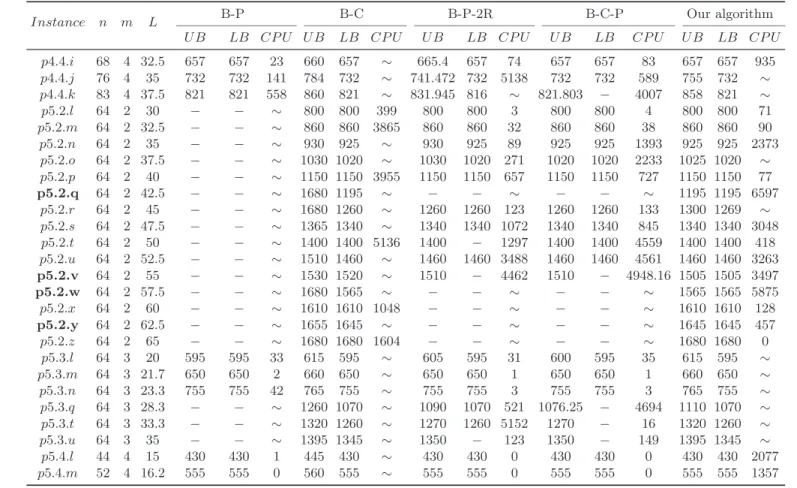
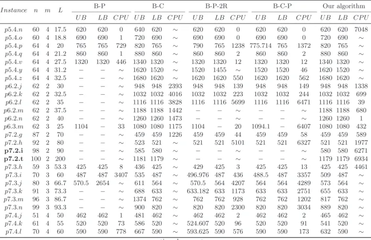
Table 3 reports the results of the instances which are solved by at least by one of the five methods (but not by all of them). In this table, columns Instance, n, m, and L respectively show the name of the instance, the number of accessible customers, the number of vehicles and the travel cost limit. Columns U B, LB, and CP U report respectively the upper bound, lower bound and computational time in seconds for each method and for each instance when available. For B-P (see Boussier et al. 2007), the reported CP U is the time spent on solving both the master problem and the subproblems until the optimality is proven. For B-C (see Dang et al. 2013a), the CP U time includes the computational times for both, the presolving and solving phases. For B-P-2R and B-C-P (see Keshtkarana et al. 2016), the CP U time is reported for the whole solving process. In our method, we consider the CP U time as the time spent in the global algorithm with the required computational time to generate the efficient cuts. For some instances, dashes “−” are used in U B and LB columns when the corresponding values were not found and tildes “∼” are used in CP U column to show that the optimalities were not proven within 7200s of the time limit.
Table 3: Comparison between our results and the literature on the standard benchmark.
Instance n m L B-P B-C B-P-2R B-C-P Our algorithm
U B LB CP U U B LB CP U U B LB CP U U B LB CP U U B LB CP U p1.2.p 30 2 37.5 250 2926 ∼ 250 250 27 250 250 15 250 250 16 250 250 7 p1.2.q 30 2 40 − − ∼ 265 265 139 265 265 78 265 265 80 265 265 5 p1.2.r 30 2 42.5 − − ∼ 280 280 33 280 280 555 280 280 566 280 280 4 p3.2.l 31 2 35 605 − 4737 590 590 53 605 590 59 591 − 2783 590 590 28 p3.2.m 31 2 37.5 − − ∼ 620 620 58 630.769 620 192 623.953 − 7121 620 620 33 p3.2.n 31 2 40 − − ∼ 660 660 48 662.453 660 1751 660 660 4345 660 660 28 p3.2.o 31 2 42.5 − − ∼ 690 690 46 699.444 690 811 699.444 − 73 690 690 19 p3.2.p 31 2 45 − − ∼ 720 720 74 730 720 3881 730 − 282 720 720 24 p3.2.q 31 2 47.5 − − ∼ 760 760 20 763.2 760 1497 763.2 − 1779 760 760 12 p3.2.r 31 2 50 − − ∼ 790 790 15 790 790 1253 790 790 1660 790 790 8 p3.2.s 31 2 52.5 − − ∼ 800 800 7 800 800 60 800 800 234 800 800 0 p3.3.s 31 3 35 738.913 416 ∼ 720 720 384 738.913 720 5136 729.36 − 5004 720 720 90 p3.3.t 31 3 36.7 763.688 4181 ∼ 760 760 257 763.688 760 157 760.693 − 2933 760 760 42 p4.2.f 98 2 50 − − ∼ − − ∼ − − ∼ − − ∼ 687 687 6550 p4.2.h 98 2 60 − − ∼ 835 835 2784 − − ∼ − − ∼ 835 835 3125 p4.2.i 98 2 65 − − ∼ 918 918 5551 − − ∼ − − ∼ 918 918 1064 p4.2.j 98 2 70 − − ∼ 969 965 ∼ − − ∼ − − ∼ 965 965 2777 p4.2.k 98 2 75 − − ∼ 1027 1022 ∼ − − ∼ − − ∼ 1022 1022 2751 p4.2.l 98 2 80 − − ∼ 1080 1074 ∼ − − ∼ − − ∼ 1074 1074 7172 p4.2.m 98 2 85 − − ∼ 1137 1132 ∼ − − ∼ − − ∼ 1132 1132 4610 p4.2.r 98 2 110 − − ∼ 1293 1292 ∼ − − ∼ − − ∼ 1292 1292 5016 p4.2.t 98 2 120 − − ∼ 1306 1306 5978 − − ∼ − − ∼ 1306 1306 0 p4.3.g 81 3 36.7 653 653 52 665 653 ∼ 656.375 653 110 653 653 306 653 653 6587 p4.3.h 90 3 40 729 729 801 761 729 ∼ 735.375 599 ∼ 730.704 − 3858 736 729 ∼ p4.3.i 94 3 43.3 809 809 4920 830 809 813.625 766 809 809 2989 815 809 1 9
Table 3 – continued from previous page
Instance n m L B-P B-C B-P-2R B-C-P Our algorithm
U B LB CP U U B LB CP U U B LB CP U U B LB CP U U B LB CP U p4.4.i 68 4 32.5 657 657 23 660 657 ∼ 665.4 657 74 657 657 83 657 657 935 p4.4.j 76 4 35 732 732 141 784 732 ∼ 741.472 732 5138 732 732 589 755 732 ∼ p4.4.k 83 4 37.5 821 821 558 860 821 ∼ 831.945 816 ∼ 821.803 − 4007 858 821 ∼ p5.2.l 64 2 30 − − ∼ 800 800 399 800 800 3 800 800 4 800 800 71 p5.2.m 64 2 32.5 − − ∼ 860 860 3865 860 860 32 860 860 38 860 860 90 p5.2.n 64 2 35 − − ∼ 930 925 ∼ 930 925 89 925 925 1393 925 925 2373 p5.2.o 64 2 37.5 − − ∼ 1030 1020 ∼ 1030 1020 271 1020 1020 2233 1025 1020 ∼ p5.2.p 64 2 40 − − ∼ 1150 1150 3955 1150 1150 657 1150 1150 727 1150 1150 77 p5.2.q 64 2 42.5 − − ∼ 1680 1195 ∼ − − ∼ − − ∼ 1195 1195 6597 p5.2.r 64 2 45 − − ∼ 1680 1260 ∼ 1260 1260 123 1260 1260 133 1300 1269 ∼ p5.2.s 64 2 47.5 − − ∼ 1365 1340 ∼ 1340 1340 1072 1340 1340 845 1340 1340 3048 p5.2.t 64 2 50 − − ∼ 1400 1400 5136 1400 − 1297 1400 1400 4559 1400 1400 418 p5.2.u 64 2 52.5 − − ∼ 1510 1460 ∼ 1460 1460 3488 1460 1460 4561 1460 1460 3263 p5.2.v 64 2 55 − − ∼ 1530 1520 ∼ 1510 − 4462 1510 − 4948.16 1505 1505 3497 p5.2.w 64 2 57.5 − − ∼ 1680 1565 ∼ − − ∼ − − ∼ 1565 1565 5875 p5.2.x 64 2 60 − − ∼ 1610 1610 1048 − − ∼ − − ∼ 1610 1610 128 p5.2.y 64 2 62.5 − − ∼ 1655 1645 ∼ − − ∼ − − ∼ 1645 1645 457 p5.2.z 64 2 65 − − ∼ 1680 1680 1604 − − ∼ − − ∼ 1680 1680 0 p5.3.l 64 3 20 595 595 33 615 595 ∼ 605 595 31 600 595 35 615 595 ∼ p5.3.m 64 3 21.7 650 650 2 660 650 ∼ 650 650 1 650 650 1 660 650 ∼ p5.3.n 64 3 23.3 755 755 42 765 755 ∼ 755 755 3 755 755 3 765 755 ∼ p5.3.q 64 3 28.3 − − ∼ 1260 1070 ∼ 1090 1070 521 1076.25 − 4694 1110 1070 ∼ p5.3.t 64 3 33.3 − − ∼ 1320 1260 ∼ 1270 1260 5152 1270 − 16 1320 1260 ∼ p5.3.u 64 3 35 − − ∼ 1395 1345 ∼ 1350 − 123 1350 − 149 1395 1345 ∼ p5.4.l 44 4 15 430 430 1 445 430 430 430 0 430 430 0 430 430 2077 2 0
Table 3 – continued from previous page
Instance n m L B-P B-C B-P-2R B-C-P Our algorithm
U B LB CP U U B LB CP U U B LB CP U U B LB CP U U B LB CP U p5.4.n 60 4 17.5 620 620 0 640 620 ∼ 620 620 0 620 620 0 620 620 7048 p5.4.o 60 4 18.8 690 690 1 720 690 ∼ 690 690 0 690 690 0 720 690 ∼ p5.4.p 64 4 20 765 765 729 820 765 ∼ 790 765 1238 775.714 765 1372 820 765 ∼ p5.4.q 64 4 21.2 860 860 1 880 860 ∼ 860 860 2 860 860 2 880 860 ∼ p5.4.v 64 4 27.5 1320 1320 446 1340 1320 ∼ 1320 1320 12 1320 1320 12 1340 1320 ∼ p5.4.y 64 4 31.2 − − ∼ 1620 1520 ∼ 1520 1455 ∼ 1520 1520 46 1620 1520 ∼ p5.4.z 64 4 32.5 − − ∼ 1680 1620 ∼ 1620 1620 550 1620 1620 562 1680 1620 ∼ p6.2.j 62 2 30 − − ∼ 948 948 2393 948 948 139 948 948 149 948 948 1338 p6.2.k 62 2 32.5 − − ∼ 1032 1032 4016 1032 1032 223 1032 1032 244 1032 1032 699 p6.2.l 62 2 35 − − ∼ 1116 1116 3828 1116 1116 5699 1116 1116 6471 1116 1116 39 p6.2.m 62 2 37.5 − − ∼ 1188 1188 1442 − − ∼ − − ∼ 1188 1188 680 p6.2.n 62 2 40 − − ∼ 1260 1260 1473 − − ∼ − − ∼ 1260 1260 1 p6.3.m 62 3 25 1104 − 33 1080 1080 1175 1104 − 20 1094.1 − 6407 1080 1080 432 p7.2.g 87 2 70 − − ∼ 459 459 1226 459 459 44 459 459 58 459 459 589 p7.2.h 92 2 80 − − ∼ 523 521 ∼ 521 521 5101 521 521 6327 521 521 1977 p7.2.i 98 2 90 − − ∼ 585 580 ∼ − − ∼ − − ∼ 580 580 6271 p7.2.t 100 2 200 − − ∼ 1181 1179 ∼ − − ∼ − − ∼ 1179 1179 6934 p7.3.h 59 3 53.3 425 425 8 436 425 ∼ 429 425 3 425 425 13 425 425 4461 p7.3.i 70 3 60 487 487 3407 535 487 ∼ 496.976 487 436 488.5 487 3357 509 487 ∼ p7.3.j 80 3 66.7 570.5 2654 ∼ 611 564 ∼ 570.5 564 4207 564 564 4289 573 564 ∼ p7.3.k 91 3 73.3 − − ∼ 688 633 ∼ 633.182 633 1173 633 633 2751 655 633 ∼ p7.3.m 96 3 86.7 − − ∼ 1374 762 ∼ 762 762 928 762 762 1202 817 762 ∼ p7.3.n 99 3 93.3 − − ∼ 900 820 ∼ 820 820 2300 820 820 3034 889 820 ∼ p7.4.j 51 4 50 462 462 1 481 462 ∼ 462 462 2 462 462 2 465 462 ∼ p7.4.k 61 4 55 520 520 73 586 520 ∼ 524.607 520 96 520 520 91 541 520 ∼ p7.4.l 70 4 60 590 590 778 667 590 593.625 590 576 590 590 173 632 590 2 1
Table 3 – continued from previous page
Instance n m L B-P B-C B-P-2R B-C-P Our algorithm
U B LB CP U U B LB CP U U B LB CP U U B LB CP U U B LB CP U
p7.4.n 87 4 70 − − ∼ 809 730 ∼ 730 730 85 730 730 95 803 730 ∼
p7.4.o 91 4 75 − − ∼ 909 781 ∼ 786.762 781 4434 784.676 − 6492 903 781 ∼
2
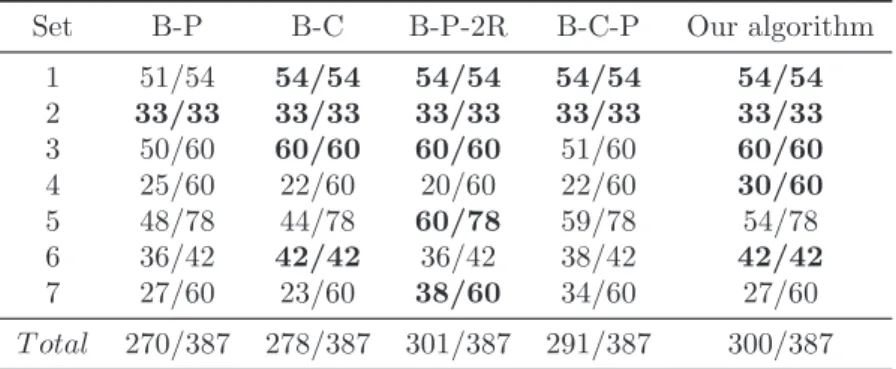
Next, we compare the performance of all the exact methods on a per-data-set basis. Table 4 summarizes the numbers of instances being solved by each method. We did not report the CP U time in this table because of some missing informations from the other methods.
Table 4: Comparison between the numbers of instances being solved by the exact methods in the literature.
Set B-P B-C B-P-2R B-C-P Our algorithm
1 51/54 54/54 54/54 54/54 54/54 2 33/33 33/33 33/33 33/33 33/33 3 50/60 60/60 60/60 51/60 60/60 4 25/60 22/60 20/60 22/60 30/60 5 48/78 44/78 60/78 59/78 54/78 6 36/42 42/42 36/42 38/42 42/42 7 27/60 23/60 38/60 34/60 27/60 T otal 270/387 278/387 301/387 291/387 300/387
A first remark from these results is that instances with large values of L and m are generally more difficult to solve than those with smaller values. This can be clearly observed with our method on the data sets 4, 5 and 7. On the other hand, none of the exact methods had a difficulty to solve the instances of the sets 1, 2, and 3, because these instances have a small numbers of accessible customers. The random distribution of customers around the depots could also make the optimal solutions easier to locate. Only a minor exception was noticed for B-P and B-C-P on some instances of the set 3.
The random distribution of customers is also the case for the sets 4 and 7, however their numbers of accessible customers are larger than those of the first three sets, e.g. they can reach 100. These large numbers cause a difficulty for all the exact methods to solve the corresponding instances. Particularly, the number of solved instances did not exceed 58 out of the 120 instances by any of the five methods.
Finally, the instances of the sets 5 and 6 contain a special geometric struc-ture. These instances have no more than 64 accessible customers, which are arranged on a grid in a way that those with large profits are far away from the depots. It appears that these instances are difficult to solve. This is especially the case with B-P and B-C algorithms. The B-P-2R and the B-C-P algorithms of Keshtkarana et al. (2016) only had problems with the set 6, while they obtained the best results for the set 5. However, our cutting-plane algorithm obtained quite good results for these two sets. It was able to solve all the instances of the set 6 and most of the instances in the set 5. We had only few difficulties with the set 5, and more precisely on some instances with 4 available vehicles. A closer look into the execution of the algorithm on those few instances revealed
to us that the CPA only made progress in improving the incumbent solution or finding equivalent ones, while it was not much reducing the upper bound.
To summarize, our algorithm was able to prove the optimality of all the instances of the sets 1, 2, 3, and 6 and a large number of instances from the other three sets. Although the instances of the set 4 are the hardest ones to solve, our CPA was able to prove the optimality of 30 out of the 60 instances, while none of the existing algorithms was able to reach that number for this set. In total, the proposed approach is capable of solving 300 out of the 387 instances.
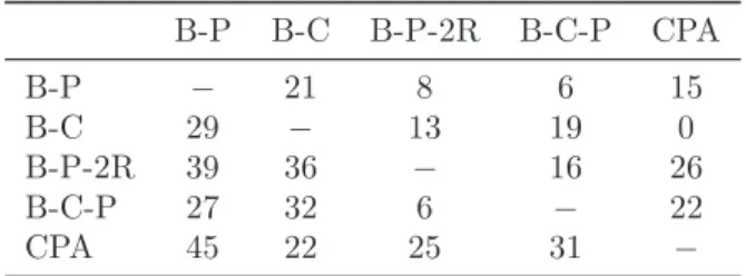
Table 5: Comparison between each two exact methods apart.
B-P B-C B-P-2R B-C-P CPA B-P − 21 8 6 15 B-C 29 − 13 19 0 B-P-2R 39 36 − 16 26 B-C-P 27 32 6 − 22 CPA 45 22 25 31 −
For further comparison between the exact methods in the literature, we present in table 5 a comparison between each two methods apart, by giving the number of instances being solved by one of the two methods and not by the other one. Each cell of this table reports the number of instances being solved by the method present in its row but not by the method in the column. From the results shown in this table, we can see that the number of instances being distinctively solved by our method is 45 compared to the B-P algorithm, 22 compared to the B-C algorithm, and respectively 25 and 31 compared to the B-P-2R and the B-C-P algorithms.
Moreover, we can notice from Table 3 that our CPA was able to improve the upper bounds of respectively 32 and 27 instances more than the two algorithms of Keshtkarana et al. (2016). Overall, our approach is clearly efficient and competitive with the existing methods in the literature. We were able to prove the optimality of 12 instances that have been unsolved in the literature. These instances are marked in bold in Table 3.
Conclusion and future work
The Team Orienteering Problem is one of the well known variants of the Vehicle Routing Problem with Profits. In this article, we presented a new ex-act algorithm to solve this problem based on a cutting-plane approach. Several types of cuts are proposed in order to strengthen the classical linear formulation. The corresponding cuts are generated and added to the model during the solv-ing process. They include symmetry breaksolv-ing, generalized subtour eliminations,
boundaries on profits/numbers of customers, forcing mandatory customers, re-moving irrelevant components and clique and independent-set cuts based on graph of incompatibilities between variables. The experiments conducted on the standard benchmark of TOP confirm the effectiveness of our approach. Our algorithm is able to solve a large number and a large variety of instances, some of those instances have been unsolved in the literature.
Interestingly, the branch-and-price algorithm of Boussier et al. (2007) and our Cutting Plane algorithm has complementary performance to each other. This gives us a hint that further development of a Branch-and-Cut-and-Price type of algorithm which incorporates our presented ideas is a promising direction towards improving the solving method for TOP. We also plan to adapt the presented approach to meet new challenges. Those could include variants of TOP on arcs, such as the Team Orienteering Arc Routing Problem (TOARP) which was addressed in (Archetti et al. 2013). On the other hand, by taking into consideration the time scheduling of the visits, the CPA can be extended to solve other variants of TOP and VRP, such as the Team Orienteering Problem with Time Windows and/or Synchronization Constraints (e.g., Labadie et al. 2012, Souffriau et al. 2013, Guibadj and Moukrim 2013, Afifi et al. 2016). Acknowledgement
This work is carried out in the framework of the Labex MS2T, which was funded by the French Government, through the program Investments for the future managed by the National Agency for Research (Reference ANR-11-IDEX-0004-02). It is also partially supported by the Regional Council of Picardie under TOURNEES SELECTIVES project and TCDU project (Collaborative Transportation in Urban Distribution, ANR-14-CE22-0017).
References
S. Afifi, D.-C. Dang, and A. Moukrim. Heuristic solutions for the vehicle routing problem with time windows and synchronized visits. Optimization Letters, 10 (3):511–525, 2016.
C. Archetti, A. Hertz, and M. Speranza. Metaheuristics for the team orienteering problem. Journal of Heuristics, 13(1):49–76, 2007.
C. Archetti, M. G. Speranza, A. Corber´an, J. M. Sanchis, and I. Planza. The team orienteering arc routing problem. Transportation Science, 48(3):442–457, 2013. C. Archetti, M. G. Speranza, and D. Vigo. Vehicle Routing Problems with Profits, chapter 10, pages 273–297. SIAM, 2014. doi: 10.1137/1.9781611973594.ch10. H. Bouly, A. Moukrim, D. Chanteur, and L. Simon. Un algorithme de
destruc-tion/construction it´eratif pour la r´esolution d’un probl`eme de tourn´ees de v´ehicules sp´ecifique. In MOSIM’08, pages 1593 – 1602, 2008.
S. Boussier, D. Feillet, and M. Gendreau. An exact algorithm for team orienteering problems. 4OR, 5(3):211–230, 2007.
S. E. Butt and T. M. Cavalier. A heuristic for the multiple tour maximum collection problem. Computers & Operations Research, 21(1):101–111, 1994.
S. E. Butt and D. M. Ryan. An optimal solution procedure for the multiple tour maximum collection problem using column generation. Computers & Operations Research, 26(4):427–441, 1999.
I.-M. Chao, B. Golden, and E. Wasil. The team orienteering problem. European Journal of Operational Research, 88:464–474, 1996.
D.-C. Dang and A. Moukrim. Subgraph extraction and metaheuristics for the maxi-mum clique problem. Journal of Heuristics, 18(5):767–794, 2012.
D.-C. Dang, R. El-Hajj, and A. Moukrim. A branch-and-cut algorithm for solving the team orienteering problem. In CPAIOR, pages 332–339, 2013a.
D.-C. Dang, R. N. Guibadj, and A. Moukrim. An effective PSO-inspired algorithm for the team orienteering problem. European Journal of Operational Research, 229(2):332–344, 2013b.
D. Feillet, P. Dejax, and M. Gendreau. Traveling salesman problems with profits. Transportation Science, 39(2):188–205, 2005.
M. Fischetti, J. J. Salazar Gonz´alez, and P. Toth. Solving the orienteering prob-lem through branch-and-cut. INFORMS Journal on Computing, 10(2):133–148, 1998.
M. Garey and D. S. Johnson. Computers and Intractability: A Guide to the Theory of NP-Completeness. W. H. Freeman and Co., 1979.
D. Gavalas, C. Konstantopoulos, and K. M. G. Pantziou. A survey on algorithmic approaches for solving tourist trip design problems. Journal of Heuristics, 20 (3):291–328, 2014.
M. Gendreau, D. Manerba, and R. Mansini. The multi-vehicle traveling purchaser problem with pairwise incompatibility constraints and unitary demands: A branch-and-price approach. European Journal of Operational Research, 248(1): 50 – 71, 2016.
R. N. Guibadj and A. Moukrim. A memetic algorithm with an efficient split procedure for the team orienteering problem with time windows. In Artificial Evolution, pages 6–17, 2013.
M. Keshtkarana, K. Ziaratia, A. Bettinellib, and D. Vigob. Enhanced exact solution methods for the team orienteering problem. International Journal of Production Research, 54(2):591 – 601, 2016.
B.-I. Kim, H. Li, and A. L. Johnson. An augmented large neighborhood search method for solving the team orienteering problem. Expert Systems with Applications, 40 (8):3065–3072, 2013.
N. Labadie, R. Mansini, J. Melechovsk´y, and R. W. Calvo. The team orienteering problem with time windows: An lp-based granular variable neighborhood search. European Journal of Operational Research, 220(1):15–27, 2012.
G. Laporte and S. Martello. The selective travelling salesman problem. Discrete Applied Mathematics, 26(2-3):193–207, 1990.
D. Manerba and R. Mansini. A branch-and-cut algorithm for the multi-vehicle travel-ing purchaser problem with pairwise incompatibility constraints. Networks, 65 (2):139 – 154, 2015.
U. Pferschy and R. Stanˇek. Using pure integer solutions to solve the traveling sales-man problem. In Middle-European Conference on Applied Theoretical Computer Science, pages 565–568, Ljubljana, Solvenia, 2013.
M. Poggi de Arag˜ao, H. Viana, and E. Uchoa. The team orienteering problem: For-mulations and branch-cut and price. In ATMOS, pages 142–155, 2010.
W. Souffriau, P. Vansteenwegen, J. Vertommen, G. Vanden Berghe, and D. Van Oud-heusen. A personalized tourist trip design algorithm for mobile tourist guides. Applied Artificial Intelligence, 22(10):964–985, 2008.
W. Souffriau, P. Vansteenwegen, G. Vanden Berghe, and D. Van Oudheusden. A path relinking approach for the team orienteering problem. Computers & Operations Research, 37(11):1853–1859, 2010.
W. Souffriau, P. Vansteenwegen, G. V. Berghe, and D. V. Oudheusden. The multicon-straint team orienteering problem with multiple time window. Transportation Science, 47(1):53–63, 2013.
H. Tang and E. Miller-Hooks. A tabu search heuristic for the team orienteering prob-lem. Computer & Operations Research, 32(6):1379–1407, 2005.
R. E. Tarjan. Depth-first search and linear graph algorithms. SIAM Journal on Computing, 1(2):146–160, 1972.
P. Vansteenwegen, W. Souffriau, G. Vanden Berghe, and D. Van Oudheusden. Meta-heuristics for tourist trip planning. In MetaMeta-heuristics in the Service Industry, volume 624 of Lecture Notes in Economics and Mathematical Systems, pages 15–31. Springer Berlin Heidelberg, 2009.
P. Vansteenwegen, W. Souffriau, and D. V. Oudheusden. The team orienteering prob-lem: A survey. European Journal of Operational Reasearch, 209:1–10, 2011.