HAL Id: hal-03214583
https://hal.archives-ouvertes.fr/hal-03214583
Submitted on 3 May 2021
HAL is a multi-disciplinary open access
archive for the deposit and dissemination of
sci-entific research documents, whether they are
pub-lished or not. The documents may come from
teaching and research institutions in France or
abroad, or from public or private research centers.
L’archive ouverte pluridisciplinaire HAL, est
destinée au dépôt et à la diffusion de documents
scientifiques de niveau recherche, publiés ou non,
émanant des établissements d’enseignement et de
recherche français ou étrangers, des laboratoires
publics ou privés.
The terrestrial carbon budget of South and Southeast
Asia
Matthew Cervarich, Shijie Shu, Atul Jain, Almut Arneth, Josep Canadell,
Pierre Friedlingstein, Richard Houghton, Etsushi Kato, Charles Koven, Prabir
Patra, et al.
To cite this version:
Matthew Cervarich, Shijie Shu, Atul Jain, Almut Arneth, Josep Canadell, et al.. The terrestrial
carbon budget of South and Southeast Asia. Environmental Research Letters, IOP Publishing, 2016,
11 (10), pp.105006. �10.1088/1748-9326/11/10/105006�. �hal-03214583�
The terrestrial carbon budget of South and
Southeast Asia
To cite this article: Matthew Cervarich et al 2016 Environ. Res. Lett. 11 105006
View the article online for updates and enhancements.
ISIMIP2a biome models
Jinfeng Chang, Philippe Ciais, Xuhui Wang et al.
Regional carbon fluxes from land use and land cover change in Asia, 1980–2009
Leonardo Calle, Josep G Canadell, Prabir Patra et al.
-Simulated carbon emissions from land-use change are substantially enhanced by accounting for agricultural management
T A M Pugh, A Arneth, S Olin et al.
-Recent citations
Pramit Kumar Deb Burman
-Seasonal variability of tropospheric CO2 over India based on model simulation, satellite retrieval and in-situ observation
M Krishnapriya et al
-Empirical estimates of regional carbon budgets imply reduced global soil heterotrophic respiration
Philippe Ciais et al
Environ. Res. Lett. 11(2016) 105006 doi:10.1088/1748-9326/11/10/105006
LETTER
The terrestrial carbon budget of South and Southeast Asia
Matthew Cervarich1, Shijie Shu1, Atul K Jain1,15, Almut Arneth2, Josep Canadell3, Pierre Friedlingstein4, Richard A Houghton5, Etsushi Kato6, Charles Koven7, Prabir Patra8, Ben Poulter9, Stephen Sitch10, Beni Stocker11, Nicolas Viovy12, Andy Wiltshire13and Ning Zeng14
1 Department of Atmospheric Sciences, University of Illinois, Urbana, IL 61801, USA
2 Karlsruhe Institute of Technology, Institute of Meteorology and Climate Research/Atmospheric Environmental Research,
Garmisch-Partenkirchen, Germany
3 Global Carbon Project, CSIRO Oceans and Atmosphere Flagship, GPO Box 3023, Canberra, ACT, 2601, Australia 4 College of Engineering, Mathematics and Physical Sciences, University of Exeter, Exeter EX4 4QF, UK
5 Woods Hole Research Center, 149 Woods Hole Road, Falmouth, MA 02540-1644, USA 6 Institute of Applied Energy, 105-0003 Tokyo, Japan
7 Earth Sciences Division, Lawrence Berkeley National Laboratory, Berkeley, CA 94720, USA 8 Department of Environmental Geochemical Cycle Research, JAMSTEC, Yokohama 2360001, Japan 9 Institute on Ecosystems and the Department of Ecology, Montana State University, Bozeman, MT 59717, USA 10 College of Life and Environmental Sciences, University of Exeter, Exeter EX4 4RJ, UK
11 Department of Life Sciences, Imperial College, Ascot SL5 7PY, UK
12 Laboratoire des sciences du climat et de l’environnement, CEA Saclay, F-91191 Gif-sur-Yvette Cedex, France 13 Met Office Hadley Centre, Fitzroy Road, Exeter EX1 3PB, UK
14 Department of Atmospheric and Oceanic Science and Earth System Science Interdisciplinary Center, University of Maryland, College
Park, MD 20742, USA
15 Author to whom any correspondence should be adressed.
E-mail:[email protected]
Keywords: terrestrial carbon, land surface model, carbon budget Supplementary material for this article is availableonline
Abstract
Accomplishing the objective of the current climate policies will require establishing carbon budget
and
flux estimates in each region and county of the globe by comparing and reconciling multiple
estimates including the observations and the results of top-down atmospheric carbon dioxide
(CO
2)
inversions and bottom-up dynamic global vegetation models. With this in view, this study synthesizes
the carbon source/sink due to net ecosystem productivity (NEP), land cover land use change (E
LUC),
fires and fossil burning (E
FIRE) for the South Asia (SA), Southeast Asia (SEA) and South and Southeast
Asia
(SSEA=SA+SEA) and each country in these regions using the multiple top-down and
bottom-up modeling results. The terrestrial net biome productivity
(NBP = NEP–E
LUC–E
FIRE)
calculated based on bottom-up models in combination with E
FIREbased on GFED4s data show net
carbon sinks of 217±147, 10±55, and 227±279 TgC yr
−1for SA, SEA, and SSEA. The top-down
models estimated NBP net carbon sinks were 20
±170, 4±90 and 24±180 TgC yr
−1. In
comparison, regional emissions from the combustion of fossil fuels were 495, 275, and 770 TgC yr
−1,
which are many times higher than the NBP sink estimates, suggesting that the contribution of the
fossil fuel emissions to the carbon budget of SSEA results in a significant net carbon source during the
2000s. When considering both NBP and fossil fuel emissions for the individual countries within the
regions, Bhutan and Laos were net carbon sinks and rest of the countries were net carbon source
during the 2000s. The relative contributions of each of the
fluxes (NBP, NEP, E
LUC, and E
FIRE, fossil
fuel emissions) to a nation’s net carbon flux varied greatly from country to country, suggesting a
heterogeneous dominant carbon
fluxes on the country-level throughout SSEA.
OPEN ACCESS
RECEIVED 7 April 2016 REVISED 6 September 2016 ACCEPTED FOR PUBLICATION 4 October 2016 PUBLISHED 19 October 2016
Original content from this work may be used under the terms of theCreative Commons Attribution 3.0
licence.
Any further distribution of this work must maintain attribution to the author(s) and the title of the work, journal citation and DOI.
1. Introduction
South and Southeast Asia(SSEA) is characterized by a faster than global average population growth and is increasing its food and energy production for the growing population by expanding agricultural land and burning more fossil fuels. A carbon budget, the net gain or loss of carbon, for this region will enable the constraining of other neighboring regionalfluxes and act as an overall constraint on the global carbon budget. A full carbon budget, as the one presented here is also important to support the development of climate mitigation policies, and project future climate change.
Geographically, SSEA occupies one of the largest areas of tropical forests. These forests account for about 20% of the potential global terrestrial net pri-mary productivity(NPP) and play an important role in regulating the Earth’s carbon cycle and climate (Tian et al2003). Studies suggest tropical land carbon fluxes exhibit, on average, a larger variability than temperate carbonfluxes (Tian et al1998, Foley et al2002, Peylin et al2005, Zeng et al2005, Ahlström et al2015), due to the influence of climatic events, such of El Niño and La Niña events on ecosystem processes, and the sub-sequent ecosystem disturbance such as large scale for-estfires (Patra et al2005). Specifically, studies suggest that enhanced sources occur during El Niño episodes and abnormal sinks during La Niña(Gérard et al1999, Jones et al2001). The large variability in land source and sinkfluxes makes it difficult to determine long-term trends in the net terrestrial carbonflux. There-fore, a better understanding of how the SSEA ecosys-tems respond to natural variability will reduce uncertainties in understanding the long-term trends and the magnitude and sign of the carbon-climate feedbacks.
The region has a history of land use land cover change(LULCC) activity such as intensive cultivation and overgrazing of pasturelands(Canadell2002) and transitioning forestland to agricultural land. Globally, SEA had the highest deforestation rate (FAO 2010) between 1990 and 2010 with the forests of SEA con-tracting in size by just less than 33 million hectares (FAO2010). A great deal of concern has been raised regarding to what extent such rapid changes in LULCC and management practices have affected the amount of carbon in vegetation, soil organic matter, and litter pools, thereby impacting the net land-atmosphere carbonflux, which is essential to ecosys-tem sustainability in SSEA.
Forestfires also contribute to the carbon budget by rapidly releasing carbon from vegetation. van der Werf et al(2010) estimated global biomass burning emitted 2.0 PgC yr−1with substantial interannual variability from 1997 to 2009. Fires caused by both natural and human sources impact biomass emission, sometimes in tandem. For example, in SEA it is economically advantageous to clear land viafire (Dennis et al2005).
Transitioning of land from tropical forest or peatland to agricultural or other commercial uses is driving SEA to have the highest deforestation rate worldwide (Langner and Siegert 2009). Langner and Siegert (2009) showed fire events are three times more fre-quent during El Niño years than non-El Niño.
Fossil fuel burning is another important source of carbon emissions. Globally, fossil fuels have emitted 9.0 PgC yr−1during 2000s and are the greatest source of carbon(Le Quéré et al2015). SSEA is also likely to have a large source of carbon emissions from the com-bustion of fossil fuels due to the rapidly expanding population and gross domestic product growth, both of which are closely related to fossil fuel emissions (Raupach et al2007).
Carbon budgets for the globe(Le Quéré et al2015), South Asia(Patra et al2013, Thompson et al2016), and SEA(Thompson et al2016) have been established. Additionally, Pan et al(2011) and Adachi et al (2011) evaluated the carbon budget of tropical forests in SEA and Tao et al(2013) estimated the carbon exchange due to changes in cropland coverage and management in SSEA. This study builds upon and extends the pre-vious budget studies by further investigating the ter-restrial carbon budget and its components for SSEA region and each country of SSEA region. By quantify-ing the country-specific terrestrial carbon budget and related carbonfluxes, this study will help to determine how much carbon is being stored or released in its for-ests and other ecosystems toward its budgeted reduc-tion in carbon dioxide. Country-level estimates are particularly relevant e.g., in the context of the 2015
Paris Climate agreement (UNFCCC 2015), which
requires quantifiable biosphere sources and sinks of carbon dioxide(CO2) and other greenhouse gases at country level in order to enable successful imple-mentation of climate policy. Further division of the sectorial carbon budget for large countries like India is desired for preparing efficient emission mitigation policy.
The specific objectives of this study are: (1) to esti-mate the terrestrial carbon budget components; net
ecosystem productivity (NEP), LULCC emission
(ELUC), and fire emissions due to non-land use change activities (EFIRE); of South Asia (SA) and Southeast Asia(SEA), the two sub-regions of SSEA, and that of each contributing country of SA(Bangladesh, Bhutan, India, Nepal, PakistanSri Lanka,) and SEA (Brunei, Cambodia, Indonesia, Laos, Malaysia, Myanmar, Phi-lippines, Singapore, Thailand, and Vietnam) regions for the period 2000–2013; (2) estimate NEP and its interannual variability for the period 1980–2013; (3) compare the terrestrial carbon budget, in terms of net biome production(NBP=NEP−ELUC−EFIRE) of SA and SEA and the countries within these two regions to the fossil fuel emissions. We use multiple data pro-ducts; including fossil fuel inventory data and remote sensing data products for EFIRE; the results of dynamic
models), atmospheric inversion models (or top-down models) and a book-keeping model to estimate the carbonfluxes and terrestrial carbon budget.
2. Data and methods
The study region is SSEA. We report here carbon fluxes for SA, SEA and entire SSEA and for those countries whose areas occupy twelve or more 0.5°×0.5° pixels, which is the standard resolution for the bottom-up models being used in this study. Singapore and Brunei are the only two countries whose areas do not satisfy our criteria; therefore we do not report carbon emissions for these two countries, but account for their carbonfluxes in regional total estimates. In the following we describe the methods and the data we used to estimate the terrestrial carbon budget(carbon sink and source terms), and the fossil fuel emissions for comparison purpose.
2.1. Net ecosystem production(NEP) and LULCC emissions estimated based on TRENDY models(or bottom-up models)
We use an ensemble of nine dynamic global vegetation
models(DGVMs: CLM4.5 Oleson et al2013, ISAM
Jain et al 2013, JULES Clark et al 2011, LPJ Sitch et al 2003, LPJ_GUESS Ahlström et al 2012, LPX Stocker et al 2014, ORCHIDEE Krinner et al2005,
VEGAS Zeng et al 2005 and VISIT Ito and
Ina-tomi 2012) results for carbon fluxes over for SSEA region. Model simulations follow the protocol as described by the carbon cycle model intercomparison project (TRENDY) (Sitch et al 2015), where each model was run from its pre-industrial equilibrium (assumed at the beginning of the 1860) to 2013. Here
we use the TRENDY model results for NEP(=NPP
(net primary productivity)—Rh (heterotrophic respiration)) based on two different simulation
sce-narios, S2 (S2 NEP) and S3 (S3 NEP). For S2
simulations, the models were forced with changing
CO2 (Dlugokencky and Tans 2014), CRU-NCEP
reanalysis climate forcing(Harris et al2014) and time-invariant pre-industrial(year 1860) HYDE land use (Klein Goldewijk et al2011) data sets over the period 1860–2013. The S3 simulations assume the same input for CO2and climate as for S2 case, but the land use varies with time based on HYDE land use data set (figure1). All models account for nitrogen deposition. Model parameterizations are summarized in table S1. For each simulation NPP and Rh are spatially inte-grated at the regional and country level for further analysis. Land use change emissions(ELUC) are esti-mated by subtracting S2 NEP from S3 NEP(S3 NEP – S2 NEP).
2.2. Fire emissions due to non-LULCC activities The ELUCterm already accounts forfire emission due to LULCC activities, such as deforestation. In order to
account forfire emissions due to non-LULCC activ-ities (EFIRE), such as lightning induced fires, we obtained carbon emissions fromfires from the Global Fire Emissions Database version 4.1, which includes smallfire burned area (GFED4s) as described in van der Werf et al(2010) but with updated burned area (Giglio et al2013). The burned area information is used as input data in a modified version of the satellite-driven Carnegie–Ames–Stanford Approach (CASA) biogeochemical model to estimate carbon emissions associated withfires, both LULCC- and non-LULCC related(see van der Werf et al2010). To calculate EFIRE, we subtract GFED4s-estimatedfire emissions due to land use change from thefire emissions due to all fire activities(land use change and non-land use related fire activities). In this way, EFIRE also accounts for emissions from peat land, which has also not been accounted for in TRENDY model results. We analyze EFIREemission data from 1997 to 2013 in this study. 2.3. Net biome production(NBP) calculated based on bottom-up modeling approach
We estimate NBP after accounting for disturbances due to LULCC and forestfire (excluding fire emissions due to deforestation) such that NBP=S2 NEP – ELUC – EFIRE. The ELUC and EFIREterms are described in sections2.1and2.2.
The variables are averaged for the 1980s, 1990s, and 2000–2013 (hereafter, referred to as the 2000s) to evaluate the change in the NEP and NBP over the past three decades. To study the impact of climate varia-bility on NEP anomalies we detrended the NEP and climate data (temperature and precipitation) by removing the linear trend. Negative NBP values
Figure 1. South and Southeast Asia(SSEA) with HYDE land cover data(Klein Goldewijk et al2011) in 1860 and 2013.
3
represent net C release to the atmosphere and positive values represent net C sequestered by the terrestrial biosphere.
2.4. Estimates of NBP based on atmospheric CO2 inverse models(or top-down models)
In order to compare TRENDY models estimated NBP for the 2000–2013 period, which uses bottom-up modeling approach, we used NBP estimates based on the following 5 atmospheric inversion or top-down
models: ACTM (Patra et al 2011), CCAM (Rayner
et al2008), GELCA (Ganshin et al2011), JMA_CDTM (Sasaki et al2003), and CarbonTracker-Europe (Peters et al2007). Atmospheric inversion models used here inferred NBP by applying Bayesian statistics to observed atmospheric CO2concentrations, the carbon flux due to fossil fuels and simulated atmospheric transport. Fossil fuelfluxes were based on data from CDIAC and PBL. The inversion models are forced with atmospheric data from JCDAS, ECMWF, NCEP2, NCEP, or JRA-25. The inverse models are run at a relatively coarse resolution(>1.8°×1.8° spatial resolution only have 11 divisions of global land) and therefore cannot be applied at the country level. 2.5. Estimates of LULCC emissions based on the bookkeeping model
Additionally, country specific LULCC emissions esti-mated based on TRENDY models are compared with a
bookkeeping method (Houghton 2003 and 2010),
which uses the following two data types to calculate annual sources and sinks of carbon from LULCC:first, rates of land use(e.g., wood harvest) and land-cover change(e.g., conversion of forest to cropland) and, second, carbon densities(MgC ha−1) in four pools of carbon: living biomass, above- and below-ground; dead biomass, including coarse woody debris; har-vested wood products; and soil organic carbon. The effects of environmental change(e.g., the concentra-tion of CO2in the atmosphere, changes in climate, and
N deposition) were not included in the defined
changes. Rates of forest growth and rates of decay varied with type of ecosystem, type of land use, and region, but they did not vary through time in response to changing environmental conditions. Changes in the areas of croplands and pastures used in bookkeeping model calculation were obtained from FAOSTAT (2015) from 1961 to 2013. After 1990, rates of deforestation and reforestation were obtained from
the FRA 2015 (FAO 2015). Earlier changes were
compiled from data and assumptions similar to those used in previous analyses(Houghton1999,2003,2010). The bookkeeping model results for SA, SEA and SSEA presented in this study are part of a new global estimate (Houghton and Nassikas2016). Although bookkeep-ing model results are available from period 1850 to 2015, we are using the results for the period
1980–2013 for comparing two modeling approaches (DGVMs and bookkeeping).
2.6. Emissions from fossil fuel consumption and cement production
We also compare country specific NBP estimates with the emissions from fossil fuel burning and cement production. Carbon emissions from fossil fuel con-sumption were retrieved from Le Quéré et al(2015), which were compiled from many sources, including the Carbon Dioxide Information Analysis Center (CDIAC) (Boden et al2015), BP statistical review of world energy the International Energy Agency(IEA), the United Nations (UN) (2014), the United States
Department of Energy (DOE), Energy Information
Administration (EIA), and more recently also the Planbureau voor de Leefomgeving(PBL) Netherlands Environmental Assessment Agency. Here the fossil fuel emissions at national and regional levels include emissions from gasflaring and cement production (US Geological Survey2013). Data is available at a country level from 1959 to 2013. In this study we analyze data from 1980 to 2013.
3. Results
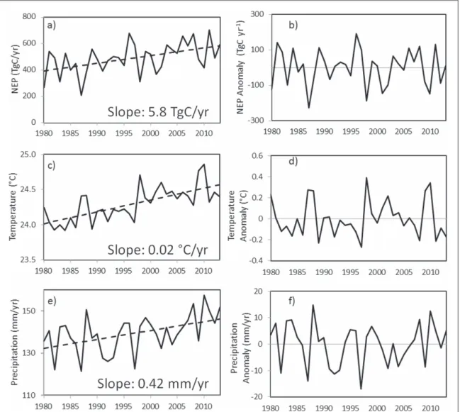
3.1. NEPThe TRENDY model results based on the S2 experi-ment, which does not consider land use change over time, suggests that NEP for SSEA increased from a sink of 414 TgC yr−1 in the 1980s to 489 TgC yr−1 and 542 TgC yr−1in the 1990s, and the 2000s, respectively, and had a 1980–2013 absolute C sink growth rate of 5.8 TgC yr−1(figures2and3(a), table S2). The increase in NEP over the period 1980–2013 has mainly been
Figure 2. Cumulative components of the terrestrial carbon budget(NEP, ELUC, EFIRE) NBP, and fossil fuels for the period
1997–2013. Positive values are a land sink of carbon and negative values are emissions to the atmosphere. Net ecosys-tem productivity(NEP; dark blue) and land use change emissions(ELUC; red) are the average of TRENDY models
estimates. Fire emission estimates due to non-land use change activities(EFIRE; green) are from the Global Fire Emissions
Database version 4(van der Werf et al2010). Net biome
productivity(NBP; solid line) is the difference between emissions from the land sink, NEP, and the land sources, ELUC, and EFIRE. Fossil fuel emission(dashed line) is sourced
from the Carbon Dioxide Information Analyses Center (CDIAC) database.
attributed to the carbon dioxide fertilization effect due to the incremental increase in atmospheric carbon dioxide concentrations (Sun et al 2014). For the 1980–2013 period, SSEA coefficient of variation (CV), the standard deviation divided by the mean, is relatively large (25%) compared to the growth rate (115 TgC yr−1) (table S2), suggesting there is substan-tial interannual variability.
All countries had positive absolute growth rates (increasing sink; decreasing source) except Bangla-desh, Bhutan, and Nepal. Bangladesh had the least absolute growth rate(−0.04 TgC yr−1) and the Indo-nesia had the greatest normalized growth rate (3 TgC yr−1) (table S2). Sri Lanka had a highest varia-tion relative to the mean as shown by a CV greater than
100% (112%), while Bangladesh had the lowest
(CV=24%) (table S2). The growth rates, which are increasing due to CO2fertilization, describe the trend in NEP, but the relatively high CVs suggest there is considerable year-to-year variability in every country.
To investigate model response to internal climate variability wefirst removed the linear trend from NEP model estimates time series (figure 3(b)), which is
influenced by non-internal climate factors, such as CO2 fertilization. We also de-trend the temperature and precipitation to remove the confounding climate change effects (figures 3(d) and (f)). The first order trend for temperature and precipitation was 0.02°C yr−1and 0.42 mm yr−1(figures3(c) and (e)). Detren-ded SSEA NEP had statistically significant correlation with detrended temperature (r=−0.71, P<0.5) (table S3) and a statistically significant correlation with detrended precipitation (r=−0.15, P>0.5) (table S3) suggesting the year to year variability in NEP was driven mainly by changes in temperature. The strong negative correlation of temperature to NEP suggests NEP in the region decreases carbon uptake or increa-ses carbon emissions in warmer years due to the increase in heterotrophic respiration in warmer envir-onments (Moncrieff and Fang 1999). Although the relationship of CO2emission and sink change with cli-mate variability is well accepted, the relative effects of
rainfall and temperature are debated (Wang
et al2014). The DGVM simulated interannual varia-tions are often much weaker than those estimated by the inverse models(e.g., Patra et al2005), suggesting
Figure 3. Interannual variation in net ecosystem productivity(NEP) (a), temperature (c), precipitation (e). Dashed lines represent least squared linearfit with slope shown in text. Detrended interannual variation in NEP (b), temperature (d), and precipitation (f).
5
that either the DGVM NEP estimates are relatively less sensitive to environmental conditions or the varia-bility of upper tropospheric CO2, which is used to drive the top-down models, is not representative variability of the boundary layer CO2which is inter-acting with the vegetation.
3.2. LULCC emissions
The TRENDY models estimated ELUCfor SSEA were a net source in the 1980s, 1990s, and 2000s with mean annual emissions of 199 TgC yr−1, 304 TgC yr−1, and 244 TgC yr−1, respectively. Every country, except Indonesia and Sri Lanka, had lower carbon emissions in the 2000s than in the 1990s(figure S1). In all three decade, Indonesia had the highest ELUCwith increas-ing trend(figure S1) and the emissions contributed to 32%, 30%, and 39% of the total SSEA emissions for the 1980s, 1990s, and 2000s, respectively. Malaysia had the second largest ELUC in the 1980s (24 TgC yr−1, 12%) and 2000s (14 TgC yr−1, 6%) (table1). In the
1990s, India had the second highest ELUC
(32 PgC yr−1, 10%). However, India experienced the greatest decrease in ELUC(26 TgC yr−1, 80%), whereas Indonesia experienced greatest increase in ELUC (3 TgC yr−1, 4%) between the 1990s and 2000s. Indonesian and Malaysian deforestation is primarily due to logging and the expansion of oil palm planta-tions (Wicke et al 2011, FAO 2010). From 1980 to 2013, 11 Mha or 6% of Indonesia’s total land area had been converted from forest to cropland(Klein Gold-ewijk et al2011). In contrast, in India reforestation/ afforestation policies practiced by India’s Ministry of the Environment and Forests in the 2000s have
decelerated the rate of deforestation (Reddy
et al2015). On the regional scale, deforestation (due to conversion of forest to cropland and pasturelands) was
the major driving factor of LULCC emission over the last three decades. The deforestation rates for SSEA region in the 1980s, 1990s, and 2000s were 1.25, 0.93, and 0.82 Mha−1. Part of the deforestation effect is compensated by the forest regrowth in the regions which were the greatest in the 1980s(0.36 Mha yr−1) (figure 4) mitigating part of the carbon emissions associated deforestation. Likewise, the 2000s had a forest regrowth of 0.16 Mha yr−1 with a majority (81%) of regrowth due to the abandonment of cropland.
The ELUC from the bookkeeping model for the 2000s are within the uncertainty range of the bottom-up models for SSEA region and for 11 of 14 countries (figure S1). Additionally, the bookkeeping model is consistent with bottom-up models with respect to the decadal trend for SSEA—an increase from the 1980s to the 1990s followed by a decrease from the 1990s to the 2000s. Differences may be due to different LULCC inputs and different modeling approaches to estimate emissions due to land use changes.
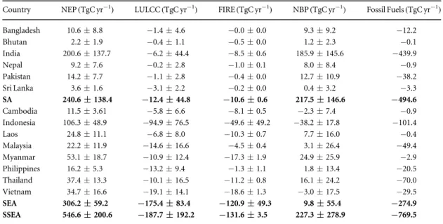
Table 1. Terrestrial carbonfluxes for the countries in South Asia (SA), Southeast Asia (SEA) and South and Southeast Asia
(SSEA= SA+SEA) (listed in alphabetic order) for the 2000–2013 period based on the average of the nine TRENDY models. NBP for SSEA for 2000–2013 Positive values are sink of carbon and negative values are source of carbon. Uncertainty is estimated with the 1-σ standard deviation from the terrestial ecosystem models. Fossil fuel emissions are from the Carbon Dioxide Information Analysis Center(CDIAC) database and averaged over the 2000–2013 period.
Country NEP(TgC yr−1) LULCC(TgC yr−1) FIRE(TgC yr−1) NBP(TgC yr−1) Fossil Fuels(TgC yr−1) Bangladesh 10.6±8.8 −1.4±4.6 −0.0±0.0 9.3±9.2 −12.2 Bhutan 2.2±1.9 −0.4±1.1 −0.5±0.0 1.2±2.3 −0.1 India 200.6±137.7 −6.2±44.4 −8.5±0.6 185.9±145.6 −439.9 Nepal 9.2±7.6 −0.2±2.8 −1.0±0.1 8.0±8.4 −0.9 Pakistan 14.2±7.7 −1.1±2.8 −0.4±0.0 12.7±10.9 −38.2 Sri Lanka 3.6±1.6 −3.1±2.2 −0.2±0.0 0.4±3.2 −3.3 SA 240.6±138.4 −12.4±44.8 −10.6±0.6 217.5±146.6 −494.6 Cambodia 11.5±3.61 −5.8±6.6 −8.1±0.5 −2.3±7.4 −0.9 Indonesia 106.3±48.9 −94.9±76.5 −49.6±49.2 −38.2±17.8 −101.4 Laos 24.8±11.1 −6.8±8.0 −10.3±0.7 7.7±16.0 −0.4 Malaysia 22.2±11.9 −14.6±16.6 −4.5±0.4 3.1±26.4 −49.4 Myanmar 53.1±18.7 −10.9±12.4 −17.3±1.9 24.9±25.9 −2.9 Philippines 16.2±5.3 −13.2±9.4 −1.3±1.1 1.8±13.4 −20.5 Thailand 37.4±13.3 −10.1±16.5 −11.2±0.8 16.1±24.2 −70.0 Vietnam 34.7±16.6 −19.1±14.1 −18.6±1.3 −3.0±17.5 −29.5 SEA 306.2±59.2 −175.4±83.4 −120.9±49.3 9.8±55.4 −274.9 SSEA 546.6±200.6 −187.7±192.2 −131.6±3.5 227.3±278.9 −769.5
Figure 4. Decadal average rate of conversions of land in South and Southeast Asia(SSEA).
3.3. Fire emissions
The estimated average SSEA EFIREfor 1997–2013 were
132±4TgC yr−1. Forest fires from Indonesia
accounted for 50±49 TgC yr−1. Indonesia employs peatlandfires as a land clearing technique before the planting of crops. Cambodia, Laos, Thailand, Myan-mar, and Vietnam collectively contribute to 31% of the region total with rates of 8±1 TgC yr−1, 10±1 TgC yr−1, 11±1 TgC yr−1, 17±1 TgC yr−1, and 18±1 TgC yr−1, respectively. These countries are the region’s maxima for lightning activity (Chris-tian et al2003) and, in conjunction with periods of low precipitation, may be one of the causes of forestfires. Additionally, man-made fires have extensively been used to clear land for agricultural and other economic purposes(Fox2000) and may have a higher tendency to spread during dry conditions. On the regional scale, rates of are decelerating at 12 TgC yr−2 (7.3% yr−1) with substantial country to country variation(figure S2). Indonesia’s emissions are estimated to be decreas-ing 14 TgC yr−2 (11.2% yr−1), whereas India’s are increasing by 1.4 TgC yr−2(0.12% yr−1). Bangladesh, Cambodia, Myanmar, Pakistan, and Sri Lanka all have rates of change of less than 1 TgC yr−1. Additionally, there is substantial year to year variability. The CV was 86% for SSEA. The large interannual variability
suggests that fire emissions are impacted by the
variables that have high interannual variations, such as precipitation. During El Nino years, a descending branch of the Walker circulation is established over the western pacific and suppresses convection in Southeast Asia(Julian and Chervin1978), resulting in a low precipitation that leads to drying of the biomass and increases the potential to ignite a fire due to lightening. Other countries also experiencefire emis-sion variability due to changes in precipitation, but the countries that experience the greatest variability have greater forest area(figure1), and therefore emit carbon duringfire events and have larger amplitudes in fire emissions.
3.4. NBP emissions
Figures5and S3 and table1show the bottom-up models estimated mean NBP for the period 2000-2013 and its components, including S2 NEP, ELUCand EFIREfor SA, SEA and SSEA regions and individual countries within SA and SEA, respectively. The bottom-up models
estimated NBP for SA, SEA and SSEA (SA+SEA)
were 217±147 TgC yr−1, 10±55 TgC yr−1, and 227±279 TgC yr−1 (1-σ standard deviation of the
9 DGVM models (table 1), compared to the
top-down estimated NBP of 20±170 TgC yr−1,
4±190 TgC yr−1 and 24±180 TgC yr−1 (1-σ stan-dard deviation of thefive inverse models). Clearly, the bottom-up models and top-down models both suggest the terrestrial biosphere for SA and SEA regions acted as a net sink for the period 2000–2013, but the sink estimated with the bottom-up models is about many
times the estimate from the atmospheric inversion models for both regions. However, the atmospheric inversion models estimate was within one standard deviation of the bottom-up models. Multi-model syntheses suggest large uncertainties in the estimated
CO2 fluxes by both the top-down and bottom-up
approaches. Contributing to the found discrepancy is the incomplete accounting of all relevant carbonfluxes inherent in these modeling approaches. For example, the budget estimated by top-down models for the Asian regions is only weakly constrained by atmospheric observations and may be reflected as weak or no increase in uptake over SSEA, as this region is largely missing atmospheric CO2measurement data(Patra et al2016). Another possible reason for the lower estimates of carbon uptake may be the underestimate of the increase in fossil fuel emissions in this region, which is assumed a posteriori and is subtracted from the total optimized CO2 flux (Thompson et al 2016). At the same time bottom-up models may have overestimated the CO2 sink amount due to overestimation of the CO2 fertiliza-tion effect, as most models do not include nitrogen and phosphorous-limitation on gross primary production, and/or the LULCC database may have underestimated rates of deforestation. Uncertainties from initial/ boundary conditions such as climate variability (mon-soons, droughts), model parameters and land use cover data can increase the inter-model variability. A recent study analyzing TRENDY project model outputs on global scale supports the large variability of the estimated land-atmosphere carbon exchange in tropical regions (figure3, Zhao et al2016).
The estimated EFIRE for SA, SEA and SEA are 11±1, 121±49 and 132±4 TgC yr−1, which are approximately the same as the estimated ELUC emis-sions for SA, but about 50 TgC yr−1lower than ELUC emissions for SEA and SSEA regions(table1), suggest-ing that ELUCemissions influence the terrestrial
car-bon budget of SEA and SSEA more than EFIRE
emissions.
Figure 5. Mean carbonfluxes for the period 2000–2013. Error bars represent thefirst standard deviation of the model results. Fire emissions due to non-LUC relatedfire activities, EFIRE, are from Global Fire Emissions Database version 4 s
(van der Werf et al2010) and fossil fuel emissions are from the
Carbon Dioxide Information Analysis Center(CDIAC) database. NEP, ELUC, and NBP are estimated from the
TRENDY models. Positive values are a land sink of carbon and negative values are emissions to the atmosphere.
7
For the 2000s period, the estimates of the carbon sink due to S2 NEP SA, SEA and SSEA are
240±45 (CV=18%), 306±83 (27%) and
547±201 TgC yr−1 (CV=37%). The estimates of ELUC for three regions are 12±45 (CV=375%),
175±83 (CV=47%) 188±192 TgC yr−1 (CV=
88%) (table1). The relatively high CV values in ELUC, particularly for SA, suggest uncertainty in estimates of NBP based on bottom-up models is, in part, caused by representation of LULCC and varying parameteriza-tions of plant function types across the numerical models.
With regard to the individual country’s terrestrial carbonfluxes, the terrestrial ecosystems of acted as a sink for atmospheric CO2with India had the greatest sink (NBP=185±146 TgC yr−1) with relatively higher estimates of NEP (201 ± 138 TgC yr−1) and lower estimates of ELUC (−6±44 TgC yr−1) and EFIRE(−9 TgC yr−1) (figure S3). On the other hand, terrestrial ecosystems of three countries in SEA acted as source. Indonesia, Cambodia and Vietnam had esti-mated NBPs that were a source of carbon(table1and figure S3), primarily due to large emissions due tofires.
Uncertainty in NBP arises from the 9 TRENDY models representing LULCC activities and NEP differ-ently. Major differences among the models are the inclusion/exclusion of carbon-nitrogen interactions, fire simulations, cropland harvest, shifting cultivation, and wood harvest and forest degradation(table S1). It is difficult to tease out relative contribution of each of the processes to the total uncertainty because con-trolled sensitivity simulations with each model are not available.
3.5. Comparison of NBPflux with fossil fuel emissions
Carbon emissions due to fossil fuel burning increased in every country within SA and SEA(figure S4). Overall, the total regional emissions(SA, SEA and SSEA) increased from the 1980s(179, 72 and 221 TgC yr−1) to the 1990s (278, 153 and 431 TgC yr−1), and from the 1990s to the 2000s(2000–2013) (493, 275 and 768 TgC yr−1). Fossil fuel emissions are largely connected to economic activity. India had the fastest absolute growth rates and Bhutan had the slowest absolute growth rates at 16 TgC yr−2, and 0.005 TgC yr−2, respectively. India, which contributed greater than half of the regions fossil fuel emissions, has expanded its gross domestic product 10-fold from 1980 to 2013(World Bank2015). SSEA fossil fuel emissions increased every year except for in 1998 when the regions GDP decreased by 32% during the East Asian Financial crisis(World Bank2015).
While the SA and SEA terrestrial biosphere during the 2000s acted as the net carbon sink for atmospheric CO2, the magnitudes of the NBP sinks for both regions are less than the magnitude of the source due to fossil fuels(table1).
India was a net source of carbon, when fossil fuel emissions (441 TgC yr−1) are also considered. In Cambodia, Laos, Myanmar, Thailand, and Vietnam (collectively called Mainland Southeast Asia (MSEA)), non-deforestationfire emissions were of similar mag-nitude or of greater magmag-nitude than fossil fuel emis-sions. This suggests the net land to atmosphere carbon emissions in MSEA is equally or more-so driven by emissions due tofires than fossil fuels. Bhutan, Laos, Myanmar, and Nepal were net sink of carbon when considering NBP and fossil fuels. NBP estimates for Myanmar are 25±26 TgC yr−1and fossil fuel emis-sions estimates are 3 TgC yr−1(table1,figure S3). The SSEA region has emissions due fossil fuel burning which are more than 4 times higher than the region’s NBP. In contrast, the varying magnitudes of carbon sources in the countries of SSEA are different from each other and different from SSEA. This suggests the carbon budget of each country is determined by fac-tors unique to the given country, possibly including land cover type, economic activity, climate, forestfire frequency, and management.
Our analysis suggests that the distribution of car-bon emissions is not homogenous for the countries that make up SA and SEA(table1). This suggests car-bon emission reduction strategies should consider the sources at the country level.
4. Discussion and summary
Our assessment of the terrestrial carbon budget and fossil fuel emissions for SSEA and its countries provides insight into the trends andfluxes of NBP and its components. Additionally, our use of fossil fuel emissions data allows us to make quantitative compar-isons between the NBP and the emission from fossil fuel burning. NBP of SSEA region was a net sink of carbon in the 2000s.
The NBP determined from the average of the nine TRENDY models’ estimates, was 227 TgC yr−1 and based on average of atmospheric inverse models is 24 TgC yr−1. In comparison, fossil fuel emissions were 700 TgC yr−1. Fossil fuel emissions grew at 27 TgC yr−2, whereas the growth of NBP sink was 9 TgC yr−2, indicating that fossil fuel emissions grew about three times faster than the growth of the NBP sink. The NBP sink is increasing steadily due to higher atmospheric CO2and its effect on plant growth(CO2fertilization effect), while atmospheric CO2 source is increasing due to ELUC, EFIREand fossil fuel emissions.
NEP, the largest component of the terrestrial car-bon budget, had an average sink of 545 TgC yr−1and grew at 12 TgC yr−2 in the 2000s. Unlike fossil fuel emissions, NEP has a large interannual variation nega-tively correlated with temperature suggesting that increased heterotrophic respiration in warm years increases carbon emissions or decreases carbon sink.
On yearly timescales, the land sink was sensitive to changes infire emissions and variations in the local temperature. Warm and dry anomalies, typically asso-ciated with El Niño events, triggered less NEP and hence weaker carbon sink. Countries in MSEA had the greatest correlation with temperature(table S2). The interannual variability of NEP is consistent with the warming of MSEA during El Niño events and asso-ciated decrease in NEP via an increase in Rh, which is particularly sensitive to temperature increases in MSEA(Zhou et al2009).
The interannual variability of NEP is greater in DGVM than in top-down models. Top-down models are driven by tropospheric CO2sampled from aircraft in the upper atmosphere. Stephens et al(2007) showed the seasonal variability of upper tropospheric CO2is less than the seasonal variability of boundary layer CO2. Further investigation is needed into interannual variability of the vertical distribution of CO2to better constrain the top-down models.
ELUC increased from the 1980s to 1990s then reversed the trend from the 1990s to the 2000s. The reversing of the trend is attributed to human and pol-icy factors such as the afforestation efforts in India. ELUCwas 244 TgC yr−1and decreased at 1.6 TgC yr−2 in the 2000s, with relatively low interannual variability suggesting the ELUCis seldom influenced by environ-mental factors. Furthermore, ELUCdecreased in nearly every country, with the exception of Laos and Indone-sia, from the 1990s to the 2000s(figure S1). Land use change practices in Indonesia have been well-docu-mented and attributed to the expansion of palm oil plantations at the expense of tropical forests (FAO2010, Wicke et al2011), and in Laos due to the expansion of agriculture, deforestation for timber, and expansion of cities(Fox and Vogler2005).
Fire emissions due to non-LULCCfire activities,
EFIRE in SSEA are primarily from Indonesia and
MSEA. In MSEA, there is a local maxima of lightening that triggers fires in vegetated areas, including for-estfires.
Considering both NBP and fossil fuels, both for SA and SEA were net sources of atmospheric CO2 (276 and 265 TgC yr−1) in the 2000s. Fossil fuel emis-sions increased at an exponential rate throughout the 2000s, simultaneously the NBP sink also increased, but at a slower rate. If the trends continue the NBP sink will further increase, but many factors may com-plicate future projections. For example, increased temperatures may further weaken the carbon sink, in terms of NEP, in the region due to the lager enhance-ment of ecosystem respiration comparing to the increment of carbon assimilation, which is expected to be water-limited under the drier future climate. LULCC has been a source over the 2000s, but this source term is shrinking in magnitude since the 1990s and therefore is helping to increase the NBP sink through the legacy effect of slower rate of defor-estation. The EFIRE emissions are approximately
constant over the last three decades(figure S2), but the emission rates may grow in the future, as the environmental conditions grow drier and hotter due to climate change.
This study presents the terrestrial carbon budget estimates, in terms of NBP, at regional and country levels. Whilefine scale carbon budget information can be used to inform decision-makers regarding car-bon management or policy-related activities, the uncertainty in estimated regional and country spe-cific NBP based on top-down and bottom-up model-ing approaches are large, represented here as the 1σ standard deviation of the model derived estimates (figures5and S3, and tables1and S2). The magni-tude of the terrestrial carbon source terms, including deforestation and other disturbances, for countries within SSEA are probably less reliable than that of the CO2emissions from fossil-fuel burning. Additional uncertainty in the carbon budget estimates arises from sinks associated with post disturbance recovery and interannual variations due to climate anomalies. Clearly, the current approaches to model carbon dynamics need improvements to account for sub-grid scale level processes and feedbacks. Future car-bon budget analyses will require data for environ-mental variables, such as LULCC activities, at higher resolutions accounting for detailed decisions on land management at a sub-national scale, given that most countries have different land classes, different modities and multiple options for managing com-modities(West et al2013). This can be accomplished by using satellite-based land products to improve spatial representation, and supported by highly accu-rate ground-based estimates. Higher resolution data in combination with extending the DGVMs to account for carbon and other nutrient dynamics at higher resolutions will be useful for informing policy decisions, because of their ability to connect carbon and other nutrient stocks andflows to ground-based physical processes.
Acknowledgments
This research was partly supported by the NASA Land
Cover and Land Use Change Program
(NNX14AD94G) and the US National Science Foun-dation(No. NSF-AGS-12-43071).
References
Adachi M, Ito A, Ishida A, Kadir W R, Ladpala P and Yamagata Y 2011 Carbon budget of tropical forests in Southeast Asia and the effects of deforestation: an approach using a process-based model andfield measurements Biogeosciences8 2635–47
Ahlström A et al 2015 The dominant role of semi-arid ecosystems in the trend and variability of the land CO2sink Science348
895–9
Ahlström A, Schurgers G, Arneth A and Smith B 2012 Robustness and uncertainty in terrestrial ecosystem carbon response to
9
CMIP5 climate change projections Environ. Res. Lett.7 044008
Boden T A, Marland G and Andres R J 2015 Global, Regional, and National Fossil-Fuel CO2Emissions(Oak Ridge, Tenn., USA:
Carbon Dioxide Information Analysis Center, Oak Ridge National Laboratory, US Department of Energy) (doi:10.3334/CDIAC/00001_V2015)
Canadell J G 2002 Land use effects on terrestrial carbon sources and sinks Sci. China C 45(suppl.) 1–9
Christian H J et al 2003 Global frequency and distribution of lightning as observed from space by the optical transient detector J. Geophys. Res.: Atmos.108 ACL-4
Clark D B et al 2011 The joint UK land environment simulator (JULES), model description: II. Carbon fluxes and vegetation dynamics Geosci. Model Develop.4 701–22
Dennis R A et al 2005 Fire, people and pixels: linking social science and remote sensing to understand underlying causes and impacts offires in Indonesia Hum. Ecology33 465–504
Dlugokencky E and Tans P 2014 Trends in atmospheric carbon dioxide, National Oceanic & Atmospheric Administration, Earth System Research Laboratory(NOAA/ESRL)(http:// esrl.noaa.gov/gmd/ccgg/trends)
FAO, U 2010 Global Forest Resource Assessment(Rome: UN Food and Agriculture Organisation)
FAO 2015 Global Forest Resource Assessment 9 pp
FAOSTAT 2015 Food and Agriculture Organization Statistics Division(http://faostat3.fao.org/home/E) (Accessed:
March 2016)
Foley J A, Botta A, Coe M T and Costa M H 2002 El Niño–Southern oscillation and the climate, ecosystems and rivers of Amazonia Glob. Biogeochem. Cycles1679–1
Fox J 2000 How blaming‘slash and burn’ farmers is deforesting mainland southeast Asia Analysis from East West Center, Report No. 47, 1601 East-West Rd, Honolulu
Fox J and Vogler J B 2005 Land-use and land-cover change in montane mainland southeast Asia Environ. Manage.36 394–403
Ganshin A et al 2011 A global coupled eulerian-lagrangian model and 1× 1 km CO Geosci. Model Develop. Discuss.4 2047–80
Gérard J C, Nemry B, Francois L M and Warnant P 1999 The interannual change of atmospheric CO2: contribution of
subtropical ecosystems? Geophys. Res. Lett.26 243–6
Giglio L, Randerson J T and Werf G R 2013 Analysis of daily, monthly, and annual burned area using the fourth‐ generation globalfire emissions database (GFED4) J. Geophys. Res.: Biogeosci.118 317–28
Harris I, Jones P D, Osborn T J and Lister D H 2014 Updated high-resolution grids of monthly climatic observations—the CRU TS3.10 Dataset Int. J. Climatol.34 623–42
Houghton R A 2003 Revised estimates of the annual netflux of carbon to the atmosphere from changes in land use and land management 1850–2000 Tellus B55 378–90
Houghton R A 2010 How well do we know theflux of CO2from
land‐use change? Tellus B62 337–51
Houghton R A, Hackler J L and Lawrence K T 1999 The US carbon budget: contributions from land-use change Science285 574–8
Houghton R A and Nassikas A A 2016 Global and regionalfluxes of carbon from land use and land-cover change 1850–2015, submitted
Ito A and Inatomi M 2012 Use of a process-based model for assessing the methane budgets of global terrestrial ecosystems and evaluation of uncertainty Biogeosciences9 759–73
Jain A K, Meiyappan P, Song Y and House J I 2013 CO2emissions
from land‐use change affected more by nitrogen cycle, than by the choice of land‐cover data Glob. Change Biol.19 2893–906
Jones A, Roberts D L, Woodage M J and Johnson C E 2001 Indirect sulphate aerosol forcing in a climate model with an interactive sulphur cycle J. Geophys. Res.: Atmos.106 20293–310
Julian P R and Chervin R M 1978 A study of the Southern oscillation and walker circulation phenomenon Mon. Weather Rev.106 1433–51
Klein Goldewijk K, Beusen A, Van Drecht G and De Vos M 2011 The HYDE 3.1 spatially explicit database of human‐induced global land‐use change over the past 12 000 years Glob. Ecology Biogeography20 73–86
Krinner G, Viovy N, de Noblet‐Ducoudré N, Ogée J, Polcher J, Friedlingstein P, Ciais P, Sitch S and Prentice I C 2005 A dynamic global vegetation model for studies of the coupled atmosphere‐biosphere system Glob. Biogeochem. Cycles19 GB1015
Langner A and Siegert F 2009 Spatiotemporalfire occurrence in Borneo over a period of 10 years Glob. Change Biol.15 48–62
Le Quéré C et al 2015 Global carbon budget 2014 Earth Syst. Sci. Data7 47–85
Moncrieff J B and Fang C 1999 A model for soil CO2production and
transport:II. Application to a Florida Pinus elliotte plantation Agric. Forest Meteorol.95 237–56
Oleson K 2013 Technical description of version 4.5 of the Community Land Model(CLM) NCAR Technical Note NCAR/TN-503+STR 420 pp (doi:10.5065/D6RR1W7M) Pan Y et al 2011 A large and persistent carbon sink in the world’s
forests Science333 988–93
Patra P K et al 2013 The carbon budget of South Asia Biogeosciences
10 513–27
Patra P K, Canadell J G, Thompson R L, Kondo M and Poulter B 2016 Sources and Sinks of Carbon Dioxide in Populous Asia, APN Project Reference: ARCP2013-01CMY-Patra/ Canadell/ (http://apn-gcr.org/resources)
Patra P K, Maksyutov S and Nakazawa T 2005 Analysis of atmospheric CO2growth rates at Mauna Loa using CO2
fluxes derived from an inverse model Tellus B57 357–65
Patra P K, Niwa Y, Schuck T J, Brenninkmeijer C A M, Machida T, Matsueda H and Sawa Y 2011 Carbon balance of South Asia constrained by passenger aircraft CO2measurements Atmos.
Chem. Phys.11 4163–75
Peters W et al 2007 An atmospheric perspective on North American carbon dioxide exchange: carbon tracker Proc. Natl Acad. Sci.
104 18925–30
Peylin P, Bousquet P, Le Quéré C, Sitch S, Friedlingstein P, McKinley G, Gruber N, Rayner P and Ciais P 2005 Multiple constraints on regional CO2flux variations over land and
oceans Glob. Biogeochem. Cycles19 GB1011
Raupach M R, Marland G, Ciais P, Le Quéré C, Canadell J G, Klepper G and Field C B 2007 Global and regional drivers of accelerating CO2emissions Proc. Natl Acad. Sci.104
10288–93
Rayner P J, Law R M, Allison C E, Francey R J, Trudinger C M and Pickett‐Heaps C 2008 Interannual variability of the global carbon cycle(1992–2005) inferred by inversion of atmospheric CO2andδ13CO2measurements Glob.
Biogeochem. Cycles22 GB3008
Reddy C S, Rajashekar G, Krishna P H, Jha C S and Dadhwal V K 2015 Multi-source and multi-date mapping of deforestation in Central India(1935–2010) and its implication on standing phytomass carbon pool Ecological Indicators57 219–27
Sasaki T, Maki T, Oohashi S and Akagi K 2003 Optimal sampling network and availability of data acquired at inland sites Global Atmosphere Watch Report Series No. 148 World
Meteorological Organization Global Atmosphere Watch pp 77–9
Sitch S et al 2015 Recent trends and drivers of regional sources and sinks of carbon dioxide Biogeosciences12 653–79
Sitch S et al 2003 Evaluation of ecosystem dynamics, plant geography and terrestrial carbon cycling in the LPJ dynamic global vegetation model Glob. Change Biol.9 161–85
Stephens B B et al 2007 Weak northern and strong tropical land carbon uptake from vertical profiles of atmospheric CO2
Science316 1732–5
Stocker B D, Feissli F, Strassmann K M, Spahni R and Joos F 2014 Past and future carbonfluxes from land use change, shifting cultivation and wood harvest Tellus B66 23188
Sun Y, Gu L, Dickinson R E, Norby R J, Pallardy S G and Hoffman F M 2014 Impact of mesophyll diffusion on estimated global land CO2fertilization Proc. Natl Acad. Sci.
111 15774–9
Tao B, Tian H, Chen G, Ren W, Lu C, Alley K D, Xu X, Liu M, Pan S and Virji H 2013 Terrestrial carbon balance in tropical Asia: contribution from cropland expansion and land management Glob. Planet. Change100 85–98
Thompson R L et al 2016 Top-down assessment of the Asian carbon budget since the mid 1990s Nat. Commun.7 10724
Tian H, Melillo J M, Kicklighter D W, McGuire A D, Helfrich J V, Moore B and VoÈroÈsmarty C J 1998 Effect of interannual climate variability on carbon storage in Amazonian ecosystems Nature396 664–7
Tian H, Melillo J M, Kicklighter D W, Pan S, Liu J, McGuire A D and Moore B 2003 Regional carbon dynamics in monsoon Asia and its implications for the global carbon cycle Glob. Planet. Change37 201–17
UNFCCC 2015 Adaptation of the Paris agreement, FCCC/CP/ 2015/L.9/Rev.1, 12 December 2015 (https://unfccc.int/ resource/docs/2015/cop21/eng/l09r01.pdf)
United Nations 2014 2011 Energy Statistics Yearbook(New York: United Nations Department for Economic and Social Information and Policy Analysis, Statistics Division) US Geological Survey 2013 Mineral Commodity Summaries 2013
(Reston, VA: US Geological Survey) 198 pp
van der Werf G R, Randerson J T, Giglio L, Collatz G J, Mu M, Kasibhatla P S, Morton D C, DeFries R S, Jin Y V and van Leeuwen T T 2010 Globalfire emissions and the contribution of deforestation, savanna, forest, agricultural, and peatfires (1997–2009) Atmos. Chem. Phys.10 11707–35
Wang X et al 2014 A two-fold increase of carbon cycle sensitivity to tropical temperature variations Nature506 212–5
West T O, Brown M E, Duren R M, Ogle S M and Moss R H 2013 Definition, capabilities and components of a terrestrial carbon monitoring system Carbon Manage.4 413–22
Wicke B, Sikkema R, Dornburg V and Faaij A 2011 Exploring land use changes and the role of palm oil production in Indonesia and Malaysia Land Use Policy28 193–206
World Bank Group 2015 World Development Indicators 2015(World Bank Publications)
Zeng N, Mariotti A and Wetzel P 2005 Terrestrial mechanisms of interannual CO2variability Glob. Biogeochem. Cycles19
GB1016
Zhao F et al 2016 Role of CO2, climate and land use in regulating the
seasonal amplitude increase of carbonfluxes in terrestrial ecosystems: a multimodel analysis Biogeosci. Discuss.2016 1–22
Zhou T, Shi P, Hui D and Luo Y 2009 Global pattern of temperature sensitivity of soil heterotrophic respiration(Q10) and its implications for carbon‐climate feedback J. Geophys. Res.: Biogeosci.114 G02016
11