HAL Id: inria-00485847
https://hal.inria.fr/inria-00485847
Submitted on 21 May 2010
HAL is a multi-disciplinary open access
archive for the deposit and dissemination of
sci-entific research documents, whether they are
pub-lished or not. The documents may come from
teaching and research institutions in France or
abroad, or from public or private research centers.
L’archive ouverte pluridisciplinaire HAL, est
destinée au dépôt et à la diffusion de documents
scientifiques de niveau recherche, publiés ou non,
émanant des établissements d’enseignement et de
recherche français ou étrangers, des laboratoires
publics ou privés.
Analysis of Failure Correlation Impact on Peer-to-Peer
Storage Systems
Olivier Dalle, Frédéric Giroire, Julian Monteiro, Stéphane Pérennes
To cite this version:
Olivier Dalle, Frédéric Giroire, Julian Monteiro, Stéphane Pérennes. Analysis of Failure
Correla-tion Impact on Peer-to-Peer Storage Systems. 9th IEEE InternaCorrela-tional Conference on Peer-to-Peer
Computing (P2P), Sep 2009, Seattle, United States. pp.184–193, �10.1109/P2P.2009.5284518�.
�inria-00485847�
Analysis of Failure Correlation Impact on
Peer-to-Peer Storage Systems
Olivier Dalle and Fr´ed´eric Giroire and Julian Monteiro and St´ephane P´erennes MASCOTTE joint project INRIA / I3S (CNRS, Univ. of Nice-Sophia), France
Email: {firstname.lastname}@sophia.inria.fr Abstract—Peer-to-peer storage systems aim to provide a
reli-able long-term storage at low cost. In such systems, peers fail continuously, hence, the necessity of self-repairing mechanisms to achieve high durability. In this paper, we propose and study analytical models that assess the bandwidth consumption and the probability to lose data of storage systems that use erasure coded redundancy. We show by simulations that the classical stochastic approach found in the literature, that models each block independently, gives a correct approximation of the system average behavior, but fails to capture its variations over time. These variations are caused by the simultaneous loss of multiple data blocks that results from a peer failing (or leaving the system). We then propose a new stochastic model based on a fluid approximation that better captures the system behavior. In addition to its expectation, it gives a correct estimation of its standard deviation. This new model is validated by simulations.
I. INTRODUCTION
In this paper, we study peer-to-peer storage systems that have high durability requirements (i.e., backup systems or long-term storage systems), like Intermemory [9], CFS [6], Farsite [4], OceanStore [11], PAST [22], Glacier [10], Total-Recall [3] or Carbonite [5]. Such distributed storage systems are prone to disk failures (or peers that permanently leave the network). Hence, redundancy data need to be introduced to ensure high durability over a long period of time. This could be done by the trivial replication of data [6], [22] or by Erasure Codes [16], [25] (e.g., Reed Solomon or Tornado) as used by some RAID schemes [18]. In the later, the system splits the user data (files, raw data, etc.) into data blocks, and then generates a set of redundant erasure coded fragments that are spread among participant peers. We focus on the analysis of systems that use Erasure Codes, as they are usually more efficient in terms of storage overhead than the replication [25]. To ensure durability, the system must have a self-repairing mechanism that maintains a minimum number of redundant fragments available in the network, even after multiple failures. Designing such a system raises fundamental questions: How much resource (bandwidth and storage space) is necessary to maintain this redundancy and to ensure a given level of reliability? What is the probability that a particular system configuration results in a data loss over a given time period?
To address those questions, we first consider a Markov Chain Model (MCM), similar to those found in the litera-ture [20], [1], [7], that represents the behavior of a single data block. This chain allows to compute the average behavior of the system accurately. Simulations confirm our analytical
results, but also indicate that the variations around the average behavior (i.e., the standard deviation) are much higher than those estimated by the MCM.
These variations are explained by the fact that when a disk failure occurs (or a peer permanently leaves the system) many data fragments are lost at the same time. This correlation induces large peaks in the bandwidth consumption. In addition, when the bandwidth is limited, those peaks tend to slow down the repairing process, resulting in data loss. Indeed, when the repairing time is longer, a damaged block is more likely to lose its remaining redundancy fragments to a point where it cannot be repaired. The consequence is that a bandwidth provisioning decision not taking into account these variations would lead to an erroneous design which in turn would introduce a risk of losing a significant amount of data.
In order to take into account this phenomenon, we propose a new stochastic Fluid Model, that does not represent a single block anymore, but the whole system. We provide a mathematical analysis of this model by giving a method to compute all the moments of its associated stationary dis-tribution. Simulations show that the Fluid Model predicts the system very well (1% margin). Moreover, this model is scalable since its complexity is proportional to the erasure code length and does not depend on the number of peers.
To the best of our knowledge, this paper is the first study to propose an analytical model that takes into account the correlations between data block failures. Along with failure correlation, we also point out the impact of disk age hetero-geneity on the system, and propose a new shuffling policy and a biased reconstruction policy to reduce this impact.
The remainder of this paper is organized as follows: after presenting the related work, we describe the system character-istics in the next section. In Section III we define the Markov Chain Model that estimates the average system behavior. We then compare this analytical model with an extensive set of simulations in Section IV, along with a discussion about its deficiencies. We then propose a Fluid Model that better captures the system variations, followed with its analysis, validation and some avenues for future research in Section V. Finally, our concluding remarks are in Section VI.
Related work.
The literature about P2P storage systems is abundant and several systems have been proposed. However, few analytical
models have been studied to estimate accurately the behav-ior of those systems (data durability, resource usage, e.g., bandwidth) and understand the trade-offs between the system parameters.
DHT based systems have been studied formally without the storage layer [14], but they have different requirements (e.g. network connectivity instead of data durability). The behavior of a storage system using full replication is studied in [20], where a Markov Chain Model is used to derive the lifetime of the system, and other practical metrics like storage and bandwidth overhead. Similarly, Datta and Aberer in [7] study analytical models for different maintenance strategies.
In [25], [15], the authors show that, in most cases, erasure codes use an order of magnitude less bandwidth and storage than replication to provide similar system durability. In [1], the authors also use a Markovian analysis to evaluate the performance of systems using Erasure codes for two different schemes of data recovery (centralized vs. distributed) and estimate the data lifetime and availability. In [8], Dimakis et al. show that other kinds of codes, as network coding, can be used to lower the system resource usage. In all these models, block failures are considered independent.
II. SYSTEMDESCRIPTION
The detailed characteristics of the studied P2P storage system are presented in this section. We consider a system designed for data archival, in this case the user data is immutable and stays for ever in the system. The peers could be desktop computers, enterprise servers or brick storage devices that stay turned on almost permanently. Furthermore, since in this paper we are not interested in studying the effects of increasing the system storage load, we make the simplifying assumption that the amount of data stored in the system is constant over the time.
Handling Churn. The system tolerates transient failures [24], where a peer can leave the system for short periods of time, as for example during restarts or power outages: If a peer stays disconnected for a time smaller than a given timeout (few hours), the system does not do anything [21]. Otherwise, the peer is considered to have failed permanently.
Permanent Peer Failures. Peers are subject to failures, mainly disk crashes. When a peer failure occurs, all the fragments stored on its disk are lost and the peer disk is replaced by a new empty disk. Following other works in the literature [20], [1], [13], these events occurs independently of one another, according to a memoryless process. We note α = 1/MT T F the probability for a given peer to experience a failure during a time step, with MTTF the Mean Time To Failure of a disk. It is important to note that if, for a single disk, this is a rare event, a system with thousands of disks continuously experiences such failures [19]. As a consequence, it is essential to the system to monitor the blocks’ state and maintain the redundancy by reconstructing lost fragments.
TABLE I
SUMMARY OF MAIN NOTATIONS.
N # of peers
s # of fragments in the initial block
r # of redundancy fragments
n = s + r # of fragments in a system block
r(b) # of remaining redundancy fragments of block b r0 reconstruction threshold value
l size of a fragment in bytes B total number of blocks in the system
τ time step of the model
α probability for a disk to failure during a time step δ(i) probability for a block at level i to lose one fragment
γ probability for a block to be reconstructed after a time step (γ = 1/θ)
Introduction of Erasure Coded redundancy. The user data is divided into user data blocks. Each user data block is, in turn, sub-divided into s equally sized fragments to which are added r fragments of redundancy, using Erasure Codes (see [16]). Each system block has then n = s+r fragments that are spread and stored on n different peers chosen at random among all peers in the system. Any subset of s fragments chosen among the initial s + r is sufficient to recover (reconstruct) the block. System monitoring. The system needs to continuously mon-itor the block’s redundancy level to decide if the repairing process needs to start. We consider systems that implement a threshold-based policy (often called Lazy Repair [3], [7]). When the number of available redundancy fragments of a block b drops to a threshold value r0, its reconstruction starts. Note that, higher threshold values mean lower probability to lose data, but higher bandwidth consumption. The case r0 = r − 1 is a special case called the eager policy, where a block is reconstructed as soon as a fragment is lost. This monitoring process can be done either in a centralized way or in a distributed way, using a Distributed Hash Table (DHT) [21].
Block Reconstruction. To rebuild a block b, a peer is chosen uniformly at random to carry out the reconstruction. It is done in three consecutive phases: in the first, retrieval, it has to download s of the remaining fragments; then, recoding, it rebuilds the block; and finally, sending, it spreads the r− r(b) missing fragments in the network. The amount of data transmitted per block is then (s + r − r(b))l in total, with r(b)the number of remaining redundancy fragments of block b and l the size of a fragment. A summary of the notations used throughout this paper is given in Table I.
Since the amount of traffic induced by the reconstruction transfers is much higher than the monitoring traffic, this later can be considered negligible here. Thus, the bandwidth consumption studied here is due solely to the reconstruction process.
III. MARKOVCHAINMODEL
In this section, we present the Markov Chain Model that we evaluate in the rest of the paper. This chain represents the behavior of P2P storage systems and models a single data
r0 0 r δ(r0) δ(r0+ 1) 1 δ(0) γ· (1 − δ(0)) γ· (1 − δ(r0)) δ(r) δ(r− 1) r− 1 r0+ 1 Dead
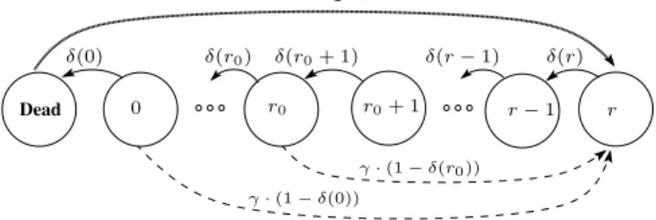
Fig. 1. Markov chain modeling the behavior of one block. Solid and dashed lines respectively represent failure and reconstruction events. Loops are omitted. Dead blocks are reinjected in the system with probability 1. block, following the approaches found in the literature [1], [7]. We derive the average values of the system behavior (probability of data loss and average bandwidth consumption) from its stationary distribution.
Markov Chain States and Transitions. The behavior of a single block is modeled by a finite discrete time Markov Chain with time step τ. The chain1(as depicted in Figure 1) has r+2 states, that represent the r + 1 levels of redundancy of a block b, and a Dead state. Three different kinds of states can be distinguished:
• Non critical: when r0+ 1 ≤ r(b) ≤ r; • Critical: when 0 ≤ r(b) ≤ r0;
• Dead: when the block has less than s fragments. A block can be affected by two different kinds of events: peer failures and reconstructions. The probability for a block at level i to lose one fragment during a time step is denoted by δ(i) and is given by
δ(i) := (s + i)α(1− α)s+i−1
(recall that α is the the probability for a peer to experience a failure during the time step). A block with no more redundancy fragments may die with probability δ(0). Note that the transi-tion time of the system, τ, can be small enough to ensure that only one disk failure happens per time step. The simultaneous loss of several fragments is emulated by successive fragment losses.
When a block becomes critical (r(b) ≤ r0), the recon-struction starts. The reconrecon-struction is modeled as follows2: the average duration of a reconstruction being noted θ, at each time step, a critical block has a probability γ := 1/θ to be rebuilt. In that case it goes to the top (r). Note that we also assume that the blocks that lose a fragment during a time step cannot be reconstructed during the same time step. If a block loses more than r(b) + 1 redundancy fragments before being reconstructed, it goes to the Dead state. In our 1For the sake of clarity, we do not describe here the most accurate and complex chain, but rather a simplified version (where unlikely transitions are ignored). They give very good approximations and provide the intuition of the system behavior. We actually use a more sophisticated chain in our computations.
2A Poisson reconstruction time is used, for mathematical tractability, and because we think it approximates well the random nature of network delays. Note that most other types of reconstruction could be captured by MCMs. For example, a reconstruction lasting a deterministic time can be modeled by labeling the states of a critical block by the progress of the reconstruction.
model, due to the stability assumption (the number of blocks is constant), a dead block is replaced immediately. This purely formal assumption does not affect the system behavior because dead blocks are rare events, but it makes the analysis more tractable.
Stationary distribution. The finite Markov chain presented above is irreducible and aperiodic. Hence, the probability to be in a state converges towards a unique stationary distribution denoted by P , where P (i) is the stationary probability to be in state i. The stationary distribution can be computed exactly in time polynomial in n by finding the eigenvector with eigenvalue 1. The complexity is independent of the number of blocks B or of the number of peers N.
Expression of the Bounds for a Simplified Chain. To give an intuition of the system behavior in function of the parameters, we present here explicit closed formulas for a simplified chain. In this chain, the probability for a block to lose a fragment is the same for all states i, given by δ = δ(r). Note that this simplified chain is “pessimistic”, in the sense that the probability to lose a fragment in any state is higher than for the former chain, and gives upper bounds for the studied metrics. For space reasons, the calculus are not shown here.
The average number of blocks lost during a time step is given by:
#dead ≈ (1 + ρρ )r0+1· δ r− r0+ ρ
B, with ρ := δ
γ(1−δ) the ratio between failure and reconstruction rates. Note that the number of dead decreases exponentially with the threshold value r0. Notice also that higher ratios of ρmean more dead.
Similarly we get the average number of blocks under reconstruction during a time step (it is the sum of blocks at level 0 ≤ i ≤ r0):
#reconstructions ≈ r ρ − r0+ ρ
B.
We see that the number of reconstructions is almost propor-tional to the inverse of r − r0. As a matter of fact, dividing r0 by 2 roughly leads to reconstruct the block after twice as many fragment losses. Note that it gives an estimation of the bandwidth needed by the system.
IV. STUDY OFCORRELATIONEFFECTS
In this section, we compare the system behavior estimated from the MCM with the results of simulations. We point out the deficiencies of the MCM to model the simultaneous loss of fragments when a disk fails. We show in Section IV-D the significant impact of this correlation on the variations of bandwidth usage, even for a large system. In Section IV-E, we examine a provisioning scenario and show that, when not taken into account, this variation could lead to a very high loss rate.
A. Simulation Model (SM)
We developed a custom cycle-based simulator to evaluate several characteristics of a real system. The simulator does not aim at capturing the low level details of the network (such as packet level communication, traffic congestion or latency), but it focuses on the global evolution of block’s states in the presence of peer failures and reconstructions.
The simulator monitors precisely the evolution of the blocks in the system, that is, their state at each time. For each disk, it stores a list of all the blocks having a fragment on it. When a disk failure occurs, the simulator updates the state of the blocks having lost a fragment. Precisely, during each cycle the simulator performs three phases:
1) generate disk failures;
2) handle the reconstruction of critical blocks:
a) for each block, test if its reconstruction is over; b) if so, choose peers randomly to spread the rebuilt
missing fragments;
3) ensure the stability of the system:
• reintroduce fragments of the dead blocks; • replace crashed disks with new empty ones. Initialization phase. At the beginning, all blocks have s + r fragments in the network (full redundancy). The fragments are uniformly distributed at random among nodes. Thus, each node starts with an average of B(s + r)/N fragments, with B the total number of blocks.
Note that during the first phase of the simulation, the system is in a transient phase. The cycles corresponding to this phase are not considered in the results given in following section. We focus on the properties of the stationary phase of the system. Monitored metrics. The main metrics monitored by the simulator are the number of reconstructions in progress (hence the bandwidth usage), the number of dead blocks, and the redundancy level of blocks (hence the number of available fragments).
At the end of each cycle, a trace is generated containing all this information. The bandwidth consumption, BW , is cal-culated using the number of on-going reconstructions during each cycle. As shown in Section II, to reconstruct a block b, the system needs to transmit (s + r − r(b))l amount of data. Thus, to estimate the total bandwidth consumption, we sum over all blocks in reconstruction, Brec, and we divide by the time step τ and by the average reconstruction cycles for one block, θ. It is assumed that the use of bandwidth is evenly distributed over the reconstruction time. We get then
BW = l· �
b∈Brec(s + r − r(b))
τ· θ .
Simulation suite and default parameters. A large number of simulations with different sets of parameters were performed. Unless otherwise explicitly indicated, the default parameter values are the following: a medium size system with N = 5000 peers (different scenarios with N spanning from 25 to
TABLE II
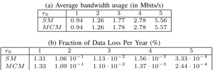
COMPARISON OF THE RESULTS OBTAINED USING THESMANDMCM,
FOR DIFFERENT VALUES OF RECONSTRUCTION THRESHOLDr0.
(a) Average bandwidth usage (in Mbits/s)
r0 1 2 3 4 5
SM 0.94 1.26 1.77 2.78 5.56
M CM 0.94 1.26 1.78 2.78 5.57
(b) Fraction of Data Loss Per Year (%)
r0 1 2 3 4 5
SM 1.31 1.06·10−1 1.13· 10−2 1.56· 10−3 3.33· 10−4
M CM 1.33 1.09·10−1 1.10· 10−2 1.37· 10−3 2.44· 10−4
1 million of peers are also evaluated); the size of a user data block is 3.6MB, thus, with s = 9 and r = 6 the size of a fragment is l = 400KB, and the system data block is 6MB (with this redundancy we have a space overhead of 66%); the reconstruction threshold value is set to r0 = 3. The system-wide number of blocks is then B = 5 · 105 (i.e., 2.86TB), which leads to an average of 600MB per disk3. Disk capacity is chosen to be 5 fold the average amount of data per disk, i.e., 3GB. The average time to reconstruct a block is θ = 12 hours. It includes the timeout delay to detect that a peer has disappeared (temporary churn) and the delay to perform the reconstruction, i.e., the time to collect the remaining fragments, to recalculate the erasure code and redistribute the missing fragments. The average lifetime of a disk or Mean Time To Failures (MTTF) is assumed to be 1 year (see e.g. [19], [23] for a discussion). In general, the simulation time Tsim was chosen to be 10 years, with a time step of one hour, which leads to 87600 cycles.
B. Average System Behavior
We compare here, for different sets of parameters, the average behavior of the system given by the Simulation Model (SM) and the one predicted from the analysis of the MCM. Table II presents a representative subset of our experiments where the value of the reconstruction threshold r0varies from 1 to 5.
We observe that the MCM gives a very precise estimation of the average bandwidth consumption (Table II-(a)) and of the fraction of data loss per year (Table II-(b)), except for values of r0 close to r. The reason is that for these values the probability to lose a block becomes very small and these values are an average over rare events.
Remark on data loss. In practice the system parameters are set in a way that the probability of a data loss is very low (e.g., in the order of 10−20). However, it is difficult to simulate such rare events in a reasonable time. To solve this issue, we deliberately chose less realistic values to evaluate the probability to lose data. In particular, the MTTF of disks was set as low as 90 days and θ raised to 24 hours.
3To be able to execute the simulations in a reasonable amount of time, we choose a system with disk size 100 times smaller than the one expected in practice As a matter of fact, to simulate 5000 peers with small disks of size 5GB, the simulator needs to deal with 30 millions of fragments. Hence, the importance to propose scalable analytical models that can accurately estimate the behavior of very large systems.
Bandwidth (Mbit/s) Frequency 0 5 10 15 0 400 800 Sim. Model Mean = 5.55 Mbits/s StdDev = 2.23 Mbits/s Bandwidth (Mbit/s) Frequency 0 5 10 15 0 10000
Markov Chain Model
Mean = 5.50 Mbits/s
StdDev = 0.10 Mbits/s
Fig. 2. Histogram of the bandwidth use by reconstructions. Top: Simulation Model. Bottom: Markov Chain Model. (Beware, y-scales are not the same.) C. The problem of correlation
Figure 2 shows an histogram with the distribution of the bandwidth consumption over time. In the top plot we have the results obtained using the Simulation Model (SM), and in the bottom, a system equivalent to the MCM, with independent fragment failures. As previously stated, the average value of both systems are very close (5.55 versus 5.50 Mbits/s). How-ever, the variations around this average are totally different. The standard deviation is 2.23 Mbits/s in the SM, to compare with only 0.1 Mbits/s in the MCM. This difference is explained by the fact that a disk failure impacts simultaneously all the blocks that have fragments stored on it. Therefore, when a failure happens, many blocks lose one fragment at the same time. Moreover, an important proportion of these blocks needs to start the reconstruction, which induces high peaks in the bandwidth consumption.
Note that the standard deviation of the independent model can be deduced directly from the MCM. Each block has a probability p = �r0
i=0P (i) of being in reconstruction, with P the stationary distribution of the MCM. Hence, the total number of blocks in reconstruction is the sum of independent variables and follows a binomial distribution of parameters B and p. This distribution is very concentrated around its mean Bpand the standard deviation is given by�Bp(1− p).
We conclude that modeling the behavior of a single block using the MCM and extrapolating the results to the whole system do not lead to an accurate representation of the system. D. Correlation and the System Size
The impact of data loss correlation shown above actually depends on the amount of fragments stored on the disk. A somewhat extreme case is when the number of peers is equal to the number of fragments of a block at full redundancy, that is N = s + r. In such a system all the blocks lose one fragment whenever a disk crashes and all the blocks follow the same trajectory. Almost at the opposite, when the disk contains few fragments (the extreme being each disk contains at most
25 50 100 250 500 1000 2500 5000 10000 25000 50000 100000 250000 500000 1000000 Sim. Model MCM Number of Peers
Bandwidth Std. Deviation (Mbits/s)
0 2 4 6 8 10 12 14
Avg. Bandwidth Mean = 1.38 Mbits/s
13 10 7.7 4.8 3.5 2.5 1.6 1.1 0.8 0.51 0.36 0.26 0.18 0.13 0.11 0.069 0.07 0.069 0.07 0.07 0.069 0.07 0.069 0.069 0.07 0.07 0.07 0.068 0.069 0.071
Fig. 3. Standard deviation of bandwidth usage versus system size. one fragment), trajectories do get independent and the system does not deviate from its mean. These two extreme examples illustrate the fact, that the impact of correlation depends on the ratio between the number of fragments per disk and the number of peers (a peer failure simultaneously impacts about (s + r)B/N fragments). In an extremely large system, the dynamic gets closer to the independent case. The following simulations confirm this intuition.
To illustrate it, we simulate systems with a fixed amount of data (same number of blocks), but with varying number of peers (between 25 and 1 million) and varying number of fragments per disk. The number of blocks is 2.5 · 105. It corresponds to 3.75 · 106 fragments. Figure 3 shows the standard deviation given by SM and MCM. The standard deviation of MCM is very far from the SM. This is obvious for small systems: 0.069 vs 7.7 for 100 peers. But this is true even for large systems: the deviation is still 5 times higher for a system with 50, 000 peers. The deviation of the dependent system decreases monotonically with the system size toward the limit obtained for the independent system. In this example, when the number of peers reaches 1 million, both standard deviations are of the same order. As expected, the standard deviation of the MCM is almost constant, as it depends only on the number of blocks which is constant here.
E. Bandwidth Provisioning and Loss of Data
We show that the data loss correlation has a strong impact on the variations of the bandwidth usage. But do these variations really affect the system reliability? What happens if the amount of bandwidth available, or allowed by the user application, is limited? To answer these questions, we simulate different scenarios with bandwidth limitation. This limit varies from µ to µ + 10σ, with µ and σ respectively the expectation and the standard deviation given by the MCM. In these experiments, when the bandwidth is not sufficient to carry out all the reconstruction demands, a queue is used to
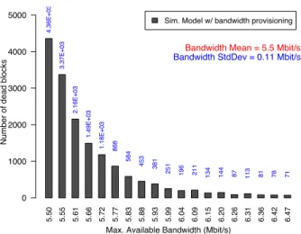
5.50 5.55 5.61 5.66 5.72 5.77 5.83 5.88 5.93 5.99 6.04 6.09 6.15 6.20 6.26 6.31 6.36 6.42 6.47
Sim. Model w/ bandwidth provisioning
Max. Available Bandwidth (Mbit/s)
Number of dead blocks
0 1000 2000 3000 4000 5000 4.36E+03 3.37E+03 2.16E+03 1.49E+03 1.18E+03 868 584 453 381 251 196 211 134 144 87 113 81 78 71
Bandwidth Mean = 5.5 Mbit/s
Bandwidth StdDev = 0.11 Mbit/s
Fig. 4. Data loss for different provisioning scenarios using the SM. store the blocks to be rebuilt. The reconstructions then start in FIFO order when bandwidth is available.
Figure 4 shows the cumulative number of dead blocks for different limits of bandwidth. We see that limiting the bandwidth has very strong impact. Between µ (5.5 Mbits/s) and µ+5σ (6.04 Mbits/s), the number of dead blocks dropped from 4.3 · 103in the former to 196 in the later. If we have no limit on the bandwidth, we also computed that the cumulative number of dead drops to 11, which is respectively 400 and 18 times less than the former cases.
Note that for all these experiments, the available bandwidth is greater than the average bandwidth given by the MCM. Hence, it is only the fact of delaying some block recon-structions that increases the probability to lose fragments. As a consequence, provisioning the system based on a model assuming block independence, as the MCM, could lead to disastrous effects. As a matter of fact, in the MCM, the bandwidth usage is very concentrated around its mean. For example, the probability to exceed µ+5σ is less than 5.810−7. A provisioning of this amount of bandwidth seems a very safe one. But as we see in Figure 4, such a dimensioning would lead to data loss. Therefore, it is very important to have a model that takes data loss correlation into account.
V. A NEWSTOCHASTICMODEL
The discussion above shows that the system cannot be seen as a set of independent blocks; so we need to model the system globally. For this purpose, we propose in this section a new approximated model based on a fluid approximation. We provide a theoretical analysis in Section V-B, giving its average behavior, the variation from its mean and a way to compute any of its moments. In Section V-C, we show by means of simulations that it models very closely the variations of a realistic system.
A. The New Model
We need to model the whole system. Block states could be fully described by a vector encoding the location of its
fragments. This would lead to a gigantic Markov Chain (with around N(s+r)B states) which is too big to compute its sta-tionary distribution. Therefore, we propose a new Markovian Approximated Model whose purpose is too approximate this gigantic chain.
The Approximated Model. The Approximated Model is derived from the following observation: fragments are spread randomly during the initialization phase and whenever a reconstruction occurs. Hence, we make the following approx-imation:
(A) At any time the fragments of a block are randomly placed into the system4.
In such a case, the state of a block is fully described by its level of redundancy and blocks at the same level are equivalent. Hence a Markov Chain that counts how many blocks are at each level can be used. The system is described by a vector B(t) = (B0(t), · · · , Br(t)) where Bi(t) is the number of blocks at level i at time t. This discrete chain can be formally described, but it is still too large for practical use (it has (r + 1)B states). However since many blocks are in the same state, we use a fluid approximation for that chain (see [12], [2] for references on fluid models).
Fluid approximation for large systems. The process to distribute the fragments among the disks follows a multinomial distribution during time (Assumption (A)). When the number of blocks B is large compared to N, as in practical systems, the multinomial distribution is very concentrated around its mean: the standard error of the number of fragments per disk is of order O(√1
B/N). The fluid approximation consists in neglecting these variations around the mean and considering that, at each time step, the proportion of blocks affected by the reconstructions and peer faults is exactly the average proportion.
We present here this stochastic Fluid Model, with discrete time step τ. The system is described by the state vector X(t) = (X0(t), · · · , Xr(t)), where Xi(t) counts the fraction of blocks that are in state i at discrete time t (i.e., X(t) = B(t)/B). The evolution of the state vector is then modelled as follows. First, we define two matrices: R, which represents the effects of the reconstruction process on the state vector,
R = 1 γ · · · γ ... 1 1− γ ... 1− γ
4Assumption (A) is indeed an approximation since the fragments of a block whose last reconstruction occurred at time T0can only be located on the disks that where in the system at time T0 and never got faulty since. The correct statement is that the fragments of a block with age T −T0are randomly spread on disks with age at least T − T0. Nevertheless we assume that (A) holds.
and F�, the effects of a disk fault, F�(t) = 1− µr(t) µ0(t) µr(t) ... ... ... ... ... µ1(t) 1− µ0(t) where µi(t) is the fraction of blocks in state i affected by a failure. We then express a transition of the system as
X(t + 1) = M (t)·X(t), with M(t) a random product defined as follows
M (t) = �
RF� with prob. f (disk fault); R with prob. 1 − f (recons. only), where f is the probability to experience a disk failure during a time step. At each time step, if no disk failure occurs, we only account for the effects of reconstructions; otherwise the disk failure effect is added. Henceforth, we note F = RF� for simplicity.
The model makes the following assumptions:
- At most one disk can fail during a time step (note that it is sufficient to choose τ small enough to ensure that multiple failures almost never happen).
- During a time step, a failure happens with probability f = αN.
- Whenever there is a failure, a block at level i has probability µi(t) to lose a fragment. This is indeed hypothesis (A). A first approach is then to consider that each disk contains a proportion 1/N of fragments (i.e., about B(s+r)/N), then the probability to lose a fragment at level i (assuming a fault) is µi(t) = s+i
N . It corresponds to a first Simple Fluid Model (SFM).
Our first simulation experiments showed that this approxima-tion already gives good results, but we can still refine it further as follows.
Disk age and number of fragments in a disk. When a disk fails, it is replaced by a new empty disk. Since disks fill up during the system life, a newly replaced disk is empty, while an old disk contains many fragments. Disk age and disk size distributions can be approximated closely for systems with large number of blocks. When a block is reconstructed, each of the rebuilt fragment is sent on a random peer. Hence, at each time step, the distribution of the rebuilt fragments among the peers follows a multinomial distribution, with parameters the number of rebuilt fragments and 1/N. As the multinomial distribution is very concentrated around its mean, the filling up process can be approximated by a affine process of its age, in which, at each time step, each disk gets in average the number of reconstructed fragments divided by the number of peers. The age of death follows a geometric law of parameter α, as at each time step a disk has a probability α to experience a fault. That is,
Pr[death age = k] = (1 − α)k−1α.
Hence, disks with very heterogeneous number of fragments are present in the system. This strong heterogeneity of the number of fragments per disk may have a significant influence on the variations of the system. As a matter of fact, when the system experiences a disk failure, we may lose a lot of fragments if the disk was almost full, but a lot less for a young disk. Therefore, we propose a refinement of the Simple Fluid Model to take these variations into account.
Fluid Model (FM). We can take the disk size distribution into account and modify µi(t) accordingly. This can be done by setting
µi(t) =(s + i)z(t)
N ,
where z(t) is the disk filling ratio and is taken according to the distribution of the numbers of fragments in a disk:
P r[z(t) = kC(α,kmax)
α ] = (1 − α)
k−1α, for 1≤ k < kmax,
P r[z(t) = kmaxC(α,kmax)
α ] = 1 − (1 − α)kmax,
where kmax and C(α, kmax) are defined below. z(t) follows a normalized truncated geometric distribution. The distribu-tion is truncated to model full disks and kmax is indirectly given by the maximum number of fragments per disk DS: DS = αkmaxB(s + r)/N, where αB(s + r) is roughly the average number of fragments reconstructed per time step. Hence, kmax represents the number of time steps to fill up a disk. The distribution is normalized to have an average filling ratio of 1: C(α, kmax)/α is the expectation of a truncated geometric distribution of parameter α for 1 ≤ k ≤ kmax. We have C(α, kmax) = 1 − (1 − α)kmax− kmax(1 − α)kmax−1+ αkmax(1 − α)kmax−1. Note that 1 is a good approximation of C for large kmax.
Note that the model is scalable since its size is s+r and the random transition matrix at time t can be computed in time O((s + r)2). Finally, let us summarize the new notations that will be used throughout this section:
f probability to have a disk failure during a time step (f = αN)
µi probability for a block in state i to be affected by a failure
B. Analysis
We present a theoretical analysis that allows to compute all the moments of the stationary distribution of the Fluid Model. The analysis boils down to the analysis of a random matrix (or matrix distribution), M(t). Note that we do not give a closed formal solution to this difficult problem because there exists no general theory to get the distribution of a random product of two matrices. It is not surprising since, for example, only determining if the infinite product of two matrices is null is an undecidable problem [17].
Expression of the expectation of the Simple Fluid Model. A transition of the system transforms the state vector X = (X1,· · · , Xn) according to
X(t + 1) = M (t)X(t). Hence,
E[X(t + 1)] = E[M(t)]E[X(t)]. The expectation of the transition matrix is given by
E[M(t)] = E[fF (t) + (1 − f)R] = fE[F (t)] + (1 − f)R, with E[F (t)] = E[RF�(t)] = RE[F�(t)], as F� is independent of R. We have E[F�(t)] = F�, with F� corresponding to the fault matrix for an average filling ratio of 1. Therefore, we obtain the same expectation for the Simple Fluid Model and the Fluid Model. To summarize, we get
E[M(t)] = fRF�+ (1 − f)R.
The linear operator E[M(t)] is a probability matrix and it can be computationally checked that 1 is the only eigenvalue with norm one. Hence we have E[X(t)] converges to E0, solution of the equation
E0= (fRF�+ (1 − f)R)E0.
Note that, since (fRF� + (1 − f)R) is roughly equivalent to the matrix transition of the MCM, we find that E[X(t)] converges to the stationary vector of the single block model. This is expected since expectations are linear.
Expression of the standard deviation of the Simple Fluid Model. We want to compute the standard deviation of the state vector X, meaning the standard deviation of each of its coordinates. We recall that each coordinate corresponds to the number of blocks in a given state.
Let start by computing E[X2].
X(t + 1)2= (M(t)X(t))2. That is Xi2= n � j1=1 mij1Xj1 � j2 mij2Xj2 . We get Xi2= � j1,j2 mij1mij2Xj1Xj2.
Note that, as X2 depends of all the cross-products of Xi and Xj, we have to compute all their expectations.
Expression of the expectations of the cross-products. We have XiXj = � n � k1=1 mik1Xk1 � � n � k2=1 mjk2Xk2 � . Hence XiXj= � k1,k2 mik1mjk2Xk1Xk2.
It gives for the expectations: E[XiXj] = E[�
k1,k2
mik1mjk2Xk1Xk2].
By linearity and independence (of mij and Xi), we obtain
E[XiXj] = �
k1,k2
E[mik1mjk2]E[Xk1Xk2].
The method is to write a linear system of equations linking the cross-product expectations at time t + 1 with the expectations at time t. Let ind be the function [1, n] × [1, n] → [1, n2], ind(i, j) = (i − 1)n + j. Let us define the matrix N by
Ni�j� = E[mi,k1mj,k2],
with i� = ind(i, j) and j�= ind(k1, k2). Note that this matrix is of dimensions n2× n2.
We now need to compute E[mi,k1mj,k2]. As the matrix of
transition M(t) is stochastic, we have to sum over all possible disk fillings z(t) to obtain the expectation. If, we note F(k) the matrix F (t) for a filling ratio equal to k, the definition of M (t)gives E[mik1mjk2] = � kmax k=1 Pr � z(t) = kC(α,kmax) α � � f Fik(k)1Fjk(k)2� +(1 − f)Rik1Rjk2.
Ni�j� is then directly derived. Now, if we note Z the vector
of the cross-products (Zind(i,j)= XiXj), we have E[Z(t + 1)] = N(t)E[Z(t)]
Again, as the linear operator E[Z(t)] is a probability matrix and because it can be checked that it has no eigenvalue with norm one other than 1, we have E[Z(t)] converges to E0, solution of the equation
E0= N(t)E0.
When Z is computed (by a resolution of a linear system with n2 variables and equations), we can extract the coefficients E[X2
i] and compute the standard deviations with σ(Xi) =�E[X2
i] − E[Xi]2.
Conclusions for the number of reconstructions and the bandwidth. The fraction of blocks in reconstruction ξ is equal to the sum of the fraction of blocks in the states from 0 to r0. We note ξ =�r0
i=0Xi. We have E[ξ] = r0 � i=0 E[Xi] and V[ξ] = r0 � i=0 r0 � j=0 cov[XiXj]. The covariances can be extracted from the previous computa-tions (cov[Xi, Xj] = E[XiXj] − E[Xi]E[Xj]).
Each reconstruction lasts in average 1/γ, translated in the model by a probability γ to be reconstructed. Hence the expectation of the bandwidth BW used by the system during one time step is
Fig. 5. Timeseries of the bandwidth used by SM and FM for 5 years.
Recall that l is the size of a fragment and s+r −r0is roughly the number of fragments sent during a reconstruction. We also get directly the variance
V[BW ] = (γ(s + r − r0)lB)2V[ξ].
Remark: Other moments can be computed similarly, albeit with additional complexity, as we need to compute all cross-products (E[X1. . . Xk] for the k-th moment).
C. Validation of the model
We run an extensive set of simulations to validate the Fluid Model (FM) for different values of parameters. Figure 5 presents an example of a timeseries of the bandwidth usage. The top plot is the Simulation Model and the bottom one the Fluid Model. As expected, the averages of the two models are almost the same (few tenths of percent). But in addition, we observe that the variations are now very close as well (2.15 Mbits/s vs. 2.23 Mbits/s).
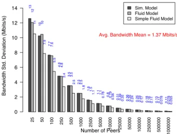
Figure 6 shows the standard deviation of the bandwidth use in both models for systems with different number of peers and fixed amount of system data. We see that the values are very close and differ by only few percents. The average bandwidth use is about the same in all these experiments and is close to 1.37 Mbits/s. Note that the variations of the FM and SFM are of the same order of magnitude, but still differ by around 20 to 40 percent in most cases, showing the impact of the heterogeneity of disk occupancy, and hence the need for the Fluid Model.
A summary of results is given in Table III. We see that the standard error of the two models differs from less than 5 percent for this set of parameters. We conclude that the system is modeled very closely by the FM.
Influence of the parameters. Note that the standard deviation does not seem to depend of the value of r0. To give an
25 50 100 250 500
1000 2500 5000 10000 25000 50000
100000 250000 500000 1000000
Sim. Model Fluid Model Simple Fluid Model
Number of Peers
Bandwidth Std. Deviation (Mbits/s)
0 2 4 6 8 10 12 14
Avg. Bandwidth Mean = 1.37 Mbits/s
13 10 7.7 4.8 3.5 2.5 1.6 1.1 0.8 0.51 0.36 0.26 0.18 0.13 0.11 12 10 7.6 4.8 3.5 2.5 1.5 1.1 0.79 0.49 0.35 0.24 0.16 0.11 0.078 11 7.9 5.5 3.4 2.5 1.8 1.1 0.78 0.56 0.35 0.24 0.17 0.11 0.078 0.055
Fig. 6. Bandwidth std. deviation vs number of peers for SM, FM (SFM is also given for comparison).
TABLE III
STANDARDERROR OFBANDWIDTH USAGE(STDDEV/MEAN)FOR
DIFFERENT VALUES OFr0, θ (IN HOURS)ANDMTTF (IN YEARS).
r0 1 2 3 4 5 SM 0.35 0.33 0.32 0.31 0.29 F M 0.31 0.31 0.31 0.30 0.29 θ 6 12 24 36 SM 0.61 0.42 0.29 0.24 F M 0.59 0.41 0.27 0.23 M T T F 1 2 3 4 5 6 8 10 SM 0.40 0.58 0.69 0.80 0.90 0.97 1.11 1.54 F M 0.38 0.55 0.67 0.78 0.87 0.96 1.09 1.66
intuition of the influence of the parameters on the system variations, we provide here a rough estimate of the standard error of the bandwidth usage. When there is a disk failure, in average, roughly RD ≈ N (r−rB(s+r)0) block reconstructions start. The average number of reconstructions can then be estimated by E[R] ≈ fRD. Let us now estimate its variance. When f is small, there are two cases: either no failure occurs with probability f and no reconstruction starts, or there is a failure and RD blocks are reconstructed. The reconstruction lasts θ time steps. Then the system reconstructs RD/θ blocks per time step during a time θ. Hence it gives V[R] ≈ (1 − fθ)E[X]2 + lθ(E[X]/fθ − E[X])2. That is V[X] ≈ (1 − fθ + fθ(1/fθ − 1)2)E[X]2 When fθ is small, we get
Std. Err.[R] ≈ √ 1 αN θ.
From this approximation, the system variations should be roughly independent of r0, but inversely proportional to√N, √
θ and proportional to√M T T F. These tendencies are seen in Table III and Figure 6.
D. Model Discussions - Future Directions
We showed that the Fluid Model closely models the be-havior of the real system. In fact, we see that the non
uniform repartition of the fragments between the different disks increases the standard deviation of the bandwidth use. To lower the impact of disk age and to have more uniform disk fillings, we propose two new policies:
• Shuffling algorithms. At each time step, a proportion of the fragments in the system are chosen at random and sent to a random disk. If all fragments are concerned, we obtain an ideal system with perfectly uniform repartition of the fragments among the disks. Note that in fact, it corresponds to the Approximated Model of Section V. The advantages of such policy are that it lowers the differences in number of fragments of the disks, but also decreases the correlation between old blocks that were more present on old disks. However, a drawback is the introduction of more network traffic in the system to redistribute the fragments.
• Biased reconstruction policy. Another way to obtain more uniform disk fillings is to change the reconstruction policy. During the last phase of the reconstruction, the rebuilt fragments are sent to random peers. We propose to choose these peers not uniformly, but to select with higher probability disks with less data. By doing so, the new disks fill up faster. One drawback of this policy, is that it reinforces the correlation between blocks rebuilt at the same time. But it has the advantage of not changing the bandwidth needs.
VI. CONCLUSION
In this paper, we study the bandwidth consumption and probability to lose data of a peer-to-peer storage system. We show through simulations and formal analysis that modeling such a system by independent blocks, each following its own Markov Chain is very far from reality: if the expectations are perfectly captured, deviations from the mean are extremely underestimated. This is due to data loss correlation: a failing disk affects tens of thousands of blocks. We also show by simulation that these variations (e.g., in bandwidth usage) can have a severe impact on the reliability (probability to lose data).
We then introduce an Approximated Fluid Model that captures most of the system dynamic. Simulations show that this model gives very tight results. We believe that the methods proposed in this paper can be applied in other contexts where correlation phenomena occur. We are working at adapting the presented methods to different (non Poissonian) failure models and different reconstruction models, e.g. deterministic reconstruction time. It could also be interesting to study data placement strategies other than random.
This work also raises a more theoretical question. The fluid models have a simple dynamic, since it is defined as a random product of two small dimension matrices. Determining the behavior of such a product is known to be intractable, but in our specific case we succeeded to get exact formulas and compute the moments of the distribution. It would be interesting to find general non trivial conditions (other than commutability) under which the dynamic can be computed.
ACKNOWLEDGMENT
This work was partially funded by the European project IST/FETAEOLUSand theANRprojects SPREADSand DIMA
-GREEN.
REFERENCES
[1] S. Alouf, A. Dandoush, and P. Nain. Performance analysis of peer-to-peer storage systems. Internation Teletraffic Congress (ITC), LNCS 4516, 4516:642–653, 2007.
[2] D. Anick, D. Mitra, and M. Sondhi. Stochastic theory of a data handling system with multiple sources. In ICC’80, volume 1, 1980.
[3] R. Bhagwan, K. Tati, Y. chung Cheng, S. Savage, and G. M. Voelker. Total recall: System support for automated availability management. In Proc. of NSDI, pages 337–350, 2004.
[4] W. J. Bolosky, J. R. Douceur, D. Ely, and M. Theimer. Feasibility of a serverless distributed file system deployed on an existing set of desktop pcs. SIGMETRICS Perform. Eval. Rev., 28(1):34–43, 2000.
[5] B.-G. Chun, F. Dabek, A. Haeberlen, E. Sit, H. Weatherspoon, M. F. Kaashoek, J. Kubiatowicz, and R. Morris. Efficient replica maintenance for distributed storage systems. In Proc. of NSDI, pages 45–48, 2006. [6] F. Dabek, M. F. Kaashoek, D. Karger, R. Morris, and I. Stoica.
Wide-area cooperative storage with CFS. In Proc. of ACM SOSP, 2001. [7] A. Datta and K. Aberer. Internet-scale storage systems under churn – a
study of the steady-state using markov models. In Intl. Conf. on Peer-to-Peer Computing (P2P), pages 133–144. IEEE Computer Society, 2006. [8] A. Dimakis, P. Godfrey, M. Wainwright, and K. Ramchandran. Network coding for distributed storage systems. In Proc. of IEEE INFOCOM, pages 2000–2008, May 2007.
[9] A. V. Goldberg and P. N. Yianilos. Towards an archival intermemory. In Proc. of ADL Conf., page 147, USA, 1998.
[10] A. Haeberlen, A. Mislove, and P. Druschel. Glacier: highly durable, decentralized storage despite massive correlated failures. In Proc. of NSDI, pages 143–158, 2005.
[11] J. Kubiatowicz, D. Bindel, Y. Chen, S. Czerwinski, P. Eaton, D. Geels, R. Gummadi, S. Rhea, H. Weatherspoon, C. Wells, et al. OceanStore: an architecture for global-scale persistent storage. ACM SIGARCH Computer Architecture News, 28(5):190–201, 2000.
[12] T. Kurtz. Approximation of Population Processes. Society for Industrial Mathematics, 1981.
[13] Q. Lian, W. Chen, and Z. Zhang. On the impact of replica placement to the reliability of distributed brick storage systems. In Proc. of ICDCS’05, volume 0, pages 187–196, 2005.
[14] D. Liben-Nowell, H. Balakrishnan, and D. Karger. Analysis of the evolution of peer-to-peer systems. In Proc. of PODC, 2002.
[15] W. Lin, D. Chiu, and Y. Lee. Erasure code replication revisited. In Proc. of P2P Computing, pages 90–97, 2004.
[16] M. Luby, M. Mitzenmacher, M. Shokrollahi, D. Spielman, and V. Ste-mann. Practical loss-resilient codes. In Proc. ACM Symp. on Theory of computing, pages 150–159, 1997.
[17] A. Markov. On the problem of representability of matrices. Z. Math. Logik Grundlagen Math, pages 157–168, 1958.
[18] D. A. Patterson, G. Gibson, and R. H. Katz. A case for redundant arrays of inexpensive disks (raid). In Proc. of ACM SIGMOD, 1988. [19] E. Pinheiro, W. Weber, and L. Barroso. Failure trends in a large disk
drive population. In Proc. of the FAST’07 Conference on File and Storage Technologies, 2007.
[20] S. Ramabhadran and J. Pasquale. Analysis of long-running replicated systems. In Proc. of INFOCOM, pages 1–9, 2006.
[21] R. Rodrigues and B. Liskov. High availability in dhts: Erasure coding vs. replication. In Peer-to-Peer Systems IV, pages 226–239. LNCS, 2005. [22] A. Rowstron and P. Druschel. Storage management and caching in past,
a large-scale, persistent peer-to-peer storage utility. In Proc. ACM SOSP, pages 188–201, 2001.
[23] B. Schroeder and G. Gibson. Disk failures in the real world: What does an mttf of 1,000,000 hours mean to you? In Proc. of the FAST’07 Conference on File and Storage Technologies, 2007.
[24] K. Tati, , K. Tati, and G. M. Voelker. On object maintenance in peer-to-peer systems. In In Proc. of the 5th International Workshop on Peer-to-Peer Systems (IPTPS), 2006.
[25] H. Weatherspoon and J. Kubiatowicz. Erasure coding vs. replication: A quantitative comparison. In Proc. of IPTPS, volume 2, pages 328–338, 2002.