HAL Id: hal-00841862
https://hal-upec-upem.archives-ouvertes.fr/hal-00841862
Submitted on 7 Jul 2013
HAL is a multi-disciplinary open access
archive for the deposit and dissemination of
sci-entific research documents, whether they are
pub-lished or not. The documents may come from
teaching and research institutions in France or
abroad, or from public or private research centers.
L’archive ouverte pluridisciplinaire HAL, est
destinée au dépôt et à la diffusion de documents
scientifiques de niveau recherche, publiés ou non,
émanant des établissements d’enseignement et de
recherche français ou étrangers, des laboratoires
publics ou privés.
Random Generation of Deterministic Acyclic Automata
Using Markov Chains
Vincent Carnino, Sven de Felice
To cite this version:
Vincent Carnino, Sven de Felice. Random Generation of Deterministic Acyclic Automata Using
Markov Chains.
Implementation and Application of Automata - 16th International Conference,
(CIAA’11), 2011, Blois, France. pp.65-75, �10.1007/978-3-642-22256-6_7�. �hal-00841862�
Random Generation of Deterministic Acyclic
Automata Using Markov Chains
Vincent Carnino and Sven De Felice⋆
LIGM, UMR 8049, Universit´e Paris-Est et CNRS, 77454 Marne-la-Vall´ee, France. [email protected],[email protected]
Abstract. In this article we propose an algorithm, based on Markov chain techniques, to generate random automata that are deterministic, accessible and acyclic. The distribution of the output approaches the uniform distribution on n-state such automata. We then show how to adapt this algorithm in order to generate minimal acyclic automata with nstates almost uniformly.
1
Introduction
In language theory, acyclic automata are exactly the automata that recognize fi-nite languages. For this reason, they play an important role in some specific fields of applications, such as the treatment of natural language. From an algorithmic point of view, they often enjoy more efficient solutions than general automata; a famous example is the linear minimization algorithm proposed by Revuz for deterministic acyclic automata [15]. They also appear as first steps in some al-gorithms, two examples of which are related to Glushkov construction [3–5] and some extension of Aho-Corasick automaton [14].
In the design and analysis of algorithms it is of great use to have access to exhaustive and random generators for the inputs of the algorithm one wants to study: the exhaustive generator is used to analyze the behavior of the algorithm for small inputs, but cannot be used for large inputs since there are too many of them; typically the number of size-n inputs often grows at least exponentially in n. Those generators can be used either to test the correctness and the efficiency of an implementation, or to help the researcher while establishing theoretical results about the average case analysis of the algorithm.
An exhaustive generator for minimal deterministic acyclic automata has been given by Almeida, Moreira and Reis [1], and in this paper we propose an algo-rithm to generate at random deterministic, accessible and acyclic automata, with a distribution that is almost uniform, using Markov chain techniques. With just a few changes, this algorithm can be turned into a generator for minimal acyclic automata. The idea is to start with a n-state acyclic automaton, then to per-form a certain amount T of mutations of this automaton, a mutation being a
⋆
The second author was supported by ANR MAGNUM - project ANR-2010-BLAN-0204.
small local transformation that preserves the required properties (deterministic, accessible and acyclic with the same number of states). Since each mutation is performed in time O(n), the complexity of our algorithm is O(nT ). The bigger T is, the more the output distribution approaches the uniform distribution. For a given distance to uniformity, it is a general difficult problem to give a good estimation of a corresponding value of T ; this is directly related to the mixing time of the Markov chain, which is generally a difficult problem [10]. Nonethe-less, the diameter of the Markov chain and the simulations we performed seems to indicate that a choice of T in Θ(n) already gives a correct random generator, at least for most applications, of complexity O(n2).
Note that the other generic methods to generate combinatorial structures uniformly at random seem to fail here. For instance, recursive methods [8] or Boltzmann samplers [7], which have been used for deterministic automata [6, 2, 9], rely on a good recursive description of the input, which is not known for acyclic automata. To our knowledge, the only combinatorial result on acyclic automata is due to Liskovets [11], who gave a close formula for the number of acyclic automata, but which cannot be directly translate into a good recursive description.
Related work:as mentioned above, our algorithm is a complement of the exhaustive generator of Almeida, Moreira and Reis [1] for testing conjectures and algorithms based on deterministic acyclic automata. The idea of using Markov chain for that kind of objects starts with works on acyclic graphs, which has been done for graph visualization purposes [12, 13]. Though using the same gen-eral idea, deterministic acyclic automata do not resemble acyclic graphs that much, mainly because they only have a linear number of edges (transitions). In particular, the diameter of the Markov chain, which is a lower bound for the mixing time, is quadratic for acyclic graphs but linear in our case. Moreover, automata considered in this article must be accessible, which is not a natural condition for graphs (there is no notion of distinguished initial vertex); Melan¸con and Philippe considered simply connected acyclic graphs in [13], but this is not the same as accessibility. For instance, they use a nice optimization based on reversing an edge, which preserves connectedness but not accessibility; hence it cannot be reused here.
The paper is organized as follows. In Section 2, we recall basic notations about automata; and in Section 3 classical Markov chain concepts are detailed. The algorithm is described in Section 4, and its correctness is given in Section 5. We present a generator for minimal acyclic automata in Section 6. Finally, in Section 7 we perform some experimentations.
2
Notations
Throughout this paper, a deterministic finite automaton is a tuple
A = (Q, A, δ, i0, F ), where Q is a finite set of states, A is a finite set of letters called the alphabet, δ : Q × A → Q is the (partial) transition function, i0 ∈ Q is the initial state and F ⊆ Q is the set of final states. In the sequel we always
suppose that |A| > 1. For any state q ∈ Q, the transition function δ(q, ·) is inductively extended to the set A∗ of all finite words over A: δ(q, ε) = q, where ε is the empty word, and for all w ∈ A∗ such that w = w1w2. . . wn, then δ(q, w) := δ(δ(. . . δ(δ(q, w1), w2) . . .), wn).
In this paper, we represent a transition δ(p, a) = q, with (p, q) ∈ Q2 and a ∈ A, by p−→ q. The notation A ⊕ pa −→ q represents the automaton A with thea additional transition p −→ q. Similarly, the notation A ⊖ pa −→ q represents thea automaton A where the transition p−→ q has been removed, if it exists.a
A state q ∈ Q is accessible (resp. co-accessible) when there exists w ∈ A∗ such that δ(i0, w) = q (resp. δ(q, w) ∈ F ). An automaton is accessible (resp. co-accessible) when all its states are accessible (resp. co-accessible).
A state q ∈ Q is transient if for all w ∈ A+, δ(q, w) 6= q. A state that is not transient is called recurrent. An automaton is acyclic when every state is transient. Another definition of acyclic automata is that the underlying directed graph is an acyclic graph. Remark that it is impossible for a complete automaton to be acyclic.
In the sequel, without loss of generality, the set of states Q of an n-state deterministic automaton will always be {1, . . . , n} and 1 will always be the ini-tial state. The size of an automaton is its number of states, and we furthermore assume from now on that n ≥ 2. Moreover, since we always consider determinis-tic, accessible and acyclic automata in this article, we shall just denote them by “acyclic automata” for short. The set of all n-state acyclic automata is denoted by An.
Also, except in Section 6, we are not considering the set of final states in our random generator. We assume that final states are chosen independently once the underlying graph of the automaton is generated.
3
Markov Chains and Random Generation
In this section we describe our algorithm to generate an acyclic automaton A of size n over the alphabet A, with the uniform probability on An. The input of algorithm is two positive integers: n, the number of states, and T , the number of iterations.
The algorithm relies on a Markov chain process: it randomly moves in the set An and returns the last automaton reached after T steps. The Markov chain of the algorithm can be seen as a directed graph whose vertices are elements of An. An edge from an automaton A to another automaton B is labelled by a real r ∈ [0, 1], which represents the probability to move from automaton A to automaton B in one step. For two automata A, B ∈ An we denote by PA,B the label of the edge from A to B, if it exists, otherwise we set PA,B= 0. Since it is a probability, we have:
∀A ∈ An, X B∈An
PA,B= 1.
A distribution on Anis a mapping p from Anto [0, 1] such thatPA∈Anp(A) =
globally unchanged after each random move, that is,
∀B ∈ An, π(B) = X A∈An
π(A) × PA,B.
A Markov Chain is called irreducible when its graph is strongly connected. For i ∈ N, let PA,B(i) be the probability to move from A to B in i steps of the algorithm. We define the period of a vertex A as the gcd of the lengths of all circuits on A: gcd({i ∈ N | PA,A(i) > 0}). If there is a loop of length 1 on A, the period of A is 1 by definition. A vertex is aperiodic if its period is 1. A Markov chain is aperiodic when all its states are aperiodic. A Markov chain is ergodic when it is both irreducible and aperiodic.
A famous property of ergodic Markov chains with a finite number of vertices is that they have a unique stationary distribution and that starting at any vertex the distribution obtained after T steps tends to this stationary distribution as T tends to infinity [10]. This gives a general framework to build a random generator on a non-empty finite set E: design an ergodic Markov chain whose set of vertex is E and such that the stationary distribution is the uniform distribution. Start from any vertex, then move randomly for a long enough time to obtain a random element of E almost uniformly.
This is exactly what we do in this article. A part of the Markov chain that is behind our algorithm is depicted in Figure 1. Each step consists either in doing nothing or in changing a transition. The complete description of the algorithm is done in Section 4. Our main result, which is proved in Section 5 is the following:
Theorem 1. The Markov chain of the algorithm is ergodic and its stationary distribution is the uniform distribution.
Since 1 is always the initial state and since there are (n − 1)! different way to label the other states there are exactly (n − 1)! automatata isomorphic to any element of An. Consequently, our uniform random generator on An yields a generator on isomorphic classes of automata which is also uniform. Note that the number of iterations T must be large enough in order to approach closely the uniform distribution. The choice of T is a difficult problem [10] and it is not entirely cover in this paper. The diameter of the Markov chain’s graph is a lower bound for T , and we will show in Section 5 that this diameter is linear in our case. In Section 7, we will see that the uniform distribution seems to be well approximated using a linear number of iterations, at least well enough for most simulation purposes.
1 2 3 1 2 3 1 2 3 1 2 3 a b b a b a, b a b a, b b 2−→ 3a 2 b − →3 1−→b 2 3−→ 2a 1−→ 2a
Fig. 1.Part of the Markov chain: at each iteration an element p −→ q of Q × A × Qa is chosen randomly. If it corresponds to a transition of the automaton, as 2−→ 3, thenb it is removed. If there is no transition labelled by a and starting at p it is added; this is the case for 2−→ 3. When there already is a transition labelled by a and startinga at p, it is redirected to q; this is the case for 1−→ 2. The mutation is not done if theb automaton is not acyclic anymore (3−→ 2) or if it is not accessible anymore (1a −→ 2).a
4
Algorithm
AcyclicAutomatonGeneration(n, T )
A ← any deterministic, accessible and acyclic automaton with n states 1
i ← 0 2
whilei < T do 3
p ← U nif orm(Q), a ← U nif orm(A), q ← U nif orm(Q \ {p}) 4 if δ(p, a) is undefined then 5 if IsAcyclic(A ⊕ p−→ q) then A = A ⊕ pa −→ qa 6 else if δ(p, a) = q then 7 if IsAccessible(A ⊖ p−→ q) then A = A ⊖ pa −→ qa 8 else 9 r ← δ(p, a) 10 if IsAccessible(A ⊖ p−→ r) thena 11 A = A ⊖ p−→ ra 12 if IsAcyclic(A ⊕ p−→ q) thena 13 A = A ⊕ p−→ qa 14 else 15 A = A ⊕ p−→ ra 16 i ← i + 1 17
Randomly choose the set of final states of A 18
returnA 19
The algorithm has two arguments: the number n of states and a value T which indicates the desired number of iterations (it is quite difficult to know when the uniform distribution is reached so it is convenient to specify it). After choosing any acyclic automaton A ∈ An to start with, the algorithm repeats the following steps T times: choose uniformly a labelled edge p−→ q with p 6= qa (p = q is not interesting since we are considering acyclic automata). Then there are three possible cases:
• There is no transition starting from p and labelled with a. In such a case, we try to add p−→ q to A and test if it is still acyclic. The transition is addeda only if it is.
• There already is a transition p−→ q in A. In that case, we test if A is stilla accessible if we remove it. If it is, the transition is removed, else A remains unchanged.
• There is a transition starting from p, labelled with a and reaching a state r, with r 6= q. In this last case, we first test whether A is still accessible if we redirect δ(p, a) to q. If it is, we do the redirection, otherwise A remains unchanged.
In this process, we need to check regularly the accessibility and the acyclicity of A.
The accessibility test is implemented the following way. We keep up-to-date, for each state q, a counter that indicates the total amount of transitions ending in q. Each time we add or remove such a transition, this counter is increased or decreased. Thus, to test the accessibility, we just have to check, after the transition has been removed, whether the counter on the state that ends the transition reaches 0 or not; this is a consequence of Lemma 1 (see Section 5). It clearly has a O(1) time complexity.
The acyclicity is tested by the classical algorithm, using a depth-first-search algorithm which runs in time O(n), since the number of transitions is linear in a deterministic automaton.
We therefore get the following result.
Proposition 1. Each iteration of the algorithm is performed in time O(n). The worst case time complexity of the algorithm is O(T n) and its space complexity is O(n).
The experimental results of Section 7 suggest that choosing T ∈ Θ(n) should be good enough; with this choice, the complexity of our algorithm would be quadratic.
5
Proofs
In this section, we prove the main facts that are used for our algorithm to correctly generate an acyclic automaton with almost uniform distribution, and with the announced complexity.
An operation which consists in removing, adding or changing a transition is called an elementary operation.
Lemma 1. Let A be an acyclic automaton of size n and B = A ⊖ p−→ q, wherea p−→ q is any transition of A. The automaton B is acyclic, and it is accessible ifa and only if there is at least one transition that ends in q in the automaton B. Proof. First note that q 6= 1, since 1 is the initial state of A, which is an acyclic and accessible automaton with at least two states.
Suppose that there is no transition that ends in q in B. Since q 6= 1, q is not accessible and neither is B.
Suppose now that B has a transition r−→ q, for some state r and some letterb b. The state r is accessible in A, and r 6= q. Since A and B only differ by a transition that ends in q, r is still accessible in B. Therefore, q is accessible in B because one can follow a path from 1 to r, then use the transition r−→ q. Sinceb all other states are accessible for the same reason as r is, B is accessible. ⊓⊔ Note that the result of Lemma 1 does not hold for automata that are not acyclic.
Lemma 2. The Markov chain of the algorithm is symmetric, that is, for all A, B ∈ An, PA,B= PB,A.
Proof. Recall that the probability to draw a given triplet (p, a, q) with p ∈ Q, q ∈ Q\{p}, and a ∈ A is 1
n(n−1)|A|. Let A, B be in An such that PA,B > 0. Then there exists an elementary operation that transforms A into B. Suppose B = A ⊕ p−→ q. The probability to draw the triplet (p, a, q) isa n(n−1)|A|1 . Now from B the only possible elementary operation to reach A is to remove the transition p−→ q. Thus, we need to draw the triplet (p, a, q) and the probabilitya of this event is 1
n(n−1)|A| too. If B = A ⊖ p a
−→ q then A = B ⊕ p−→ q thus wea are in the same case as above and PA,B = PB,A.
Suppose the elementary operation that transforms A to B is to redirect the transition p −→ q of A to obtain pa −→ s in B. To get this, we need to draw thea triplet (p, a, s) and the probability of this event is n(n−1)|A|1 = PA,B. The only possible elementary operation to reach A from B is to redirect the new transition p−→ s to pa −→ q which has the same probability, for the same reasons. Hencea PA,B= PB,A in this case too. ⊓⊔
Lemma 3. The Markov chain of the algorithm is ergodic. Proof. We need to prove that it is both irreducible and aperiodic.
To prove the irreducibility, we show that, in the Markov chain, there is a path from any acyclic automaton A ∈ An to an automaton Sn∈ An, where Sn is the acyclic automaton whose only transitions are i−→ i + 1, for i ∈ {1, . . . , n − 1}:a
1 a 2 a a n− 1 a n
Let A be any acyclic automaton and let a be a letter in A. Let E be the set of states that are accessible from the initial state by reading only a’s. E is not empty since it contains at least the initial state 1. Repeatedly remove every transition p−→ q where q ∈ E and p /α ∈ E. Then repeatedly remove every remaining transition p −→ q where p, q ∈ E and α 6= a. This actions are validα moves in the Markov chain by Lemma 1 since we always keep the transitions p−→ q with p, q ∈ E. Let ℓ be the only state in E with no outgoing transitiona labelled with a.
If |E| < n, choose a state s of A that is not in E and add a transition ℓ−→ s.a Because there is no path between s and a state of E, this operation cannot create a cycle. Repeatedly remove all transitions directed toward s except ℓ−→ s. Adda s to E, the set E is one state bigger. The size of E being finite, this operations can be repeated until E contains all states of A.
Hence, at some point |E| = n and A is isomorph to Sn, since every state but the initial one has exactly one incoming transition, which is labelled by a. The only difference with Snis that the states are not necessarily in the correct order. We now explain how they can be re-ordered.
Let b ∈ A, b 6= a for each transition p−→ q of A, we add to A the transitiona p−→ q by elementary operations, which do not create any cycle. Now we removeb all transitions labelled by a, A remains accessible because of the transitions
labelled by b. We are in the case |E| < n above, where the set E contains the state 1 only. To reach the automaton Sn, it is sufficient to choose the new states added to E in the order of their label. After removing all transitions labelled by b, we finally obtain the automaton Sn.
Hence for every A ∈ An, there exists a path from A to Sn in the Markov chain. By Lemma 2 there also exists a path from Sn to A: the Markov chain is therefore irreducible. For every automaton A ∈ An and any state p 6= 1 and any letter a ∈ A, if the edge chosen by the algorithm is (p, a, 1) then A remains the same: adding the transitions would make A cyclic. Hence every vertex has a loop of length 1 in the Markov chain, it is therefore aperiodic. ⊓⊔ Lemma 4. The diameter of the Markov chain is in Θ(n).
Proof. Using the construction proposed in the proof of Lemma 3, every A ∈ An is at distance at most (|A| + 5)n of Sn. The diameter of the Markov chain is thus at most 2(|A| + 5)n, which is O(n). The lower bound in Ω(n) is obtained by considering the distance from Sn to an acyclic automaton whose edges are all labelled by a letter b 6= a. ⊓⊔ Theorem 1 is a consequence of the lemmas above: By Lemma 3 the Markov chain of the algorithm is ergodic and by Lemma 2 it is symmetric. According to a classical result in Markov chain theory [10], its stationary distribution is the uniform distribution on An.
6
Minimal Acyclic Automata
In this section we briefly describe how to adapt our algorithm in order to generate minimal acyclic automata. Due to the lack of place, we do not give all the details here, but the adaptation is quite straightforward.
An acyclic automaton A of Anis a hammock acyclic automaton (or hammock automaton for short) if A has only one state with no outgoing transition. This state is called the target state of the hammock automaton. We denote by Hn⊂ An the set of size-n hammock automaton whose target state is n.
Our random generator can readily be adapted to generate elements of Hn: never choose p = n, in order to keep n without outgoing transition, and do not perform a deletion of p−→ q if it is the only outgoing transition of p.a
Adapting the proof of Lemma 3 to hammock automata, we can prove that the Markov chain is still ergodic and symmetric. Its stationary distribution is therefore the uniform distribution on Hn. The diameter is also in Θ(n) for this new chain.
Let Mn denote the set of minimal acyclic automata with n states. One can verify that such an automaton is necessarily an hammock automaton whose target state is final. This is of course not a sufficient condition. However, we can use this property to generate elements of Mn using a rejection algorithm: repeatedly draw a random hammock automaton (whose target state is final) until the automaton is minimal. This pseudo-algorithm may never halt, but if
the proportion of minimal automata is large enough, the average number of rejections is polynomial or even bounded above by a constant. The important point is that no bias is introduced by this method: if hammock automata are generated uniformly at random, the induced probability on the output is the uniform distribution on Mn.
We have no asymptotic result yet about the proportion of minimal automata amongst hammock automata. This may be a difficult problem, since it is still open for general deterministic automata. But experiments indicate that this proportion should be non-negligible: amongst 1000 random hammock automata of size 100, on a two-letter alphabet, we found 758 minimal automata. If we accept the conjecture that the proportion of minimal automata is at least c > 0, this yields a random generator for minimal acyclic automata with no increase of complexity, in average: the average number of rejections is bounded from above by a constant, and the test of minimality is linear, using Revuz algorithm [15].
7
Experiments
In this section, we present some experiments we did in order to evaluate the rate of convergence of our algorithm as T grows. For this purpose we use the Kolmogorov-Smirnov statistic test, which, roughly speaking, computes a value that measures the distance to the uniform distribution. This testing protocol is limited to small values of n: we need to store, for each isomorphism class of An the number of times it has been generated when performing a large number N of random generations. For the test to be meaningful, all isomorphism classes of An must have been generated, and there are many of them, even for small values of n [11, 1].
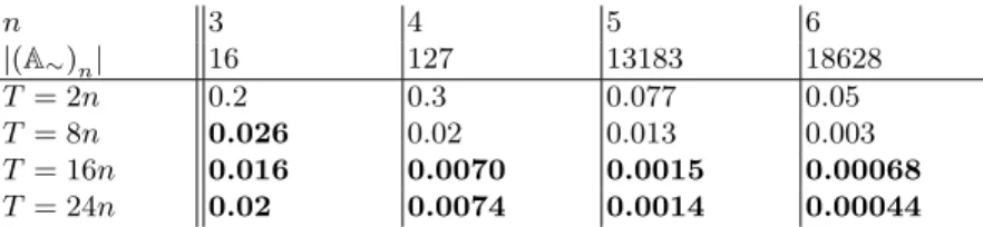
We generated a large number of acyclic automata with our generator and reported the value of the Kolmogorov-Smirnov statistic test. The results are given in Figure 2 below.
n 3 4 5 6 |(A∼)n| 16 127 13183 18628 T = 2n 0.2 0.3 0.077 0.05 T = 8n 0.026 0.02 0.013 0.003 T = 16n 0.016 0.0070 0.0015 0.00068 T = 24n 0.02 0.0074 0.0014 0.00044
Fig. 2.The values of the uniform Kolmogorov-Smirnov statistic test depending on n and of the number T of iterations in the algorithm. The tests are performed on a population of 100|(A∼)n| automata generated by the algorithm, where (A∼)n is the
set of isomorphism classes of An. We indicated in bold when the test of uniformity is
8
Conclusion
Our random generators are already usable in practice, and easy to implement. Two questions remain to justify fully their good behavior, which are ongoing works:
• The complete analysis of the main algorithm requires a good estimation of the mixing time of the underlying Markov chain.
• The efficiency of our algorithm that generates minimal acyclic automata re-lies on an estimation of the proportion of minimal automata amongst ham-mock automata.
Acknowledgement:we would like to thanks Cyril Nicaud for his precious help in most stages of this work.
References
1. Marco Almeida, Nelma Moreira, and Rog´erio Reis. Exact generation of minimal acyclic deterministic finite automata. Int. J. Found. Comput. Sci., 19(4):751–765, 2008.
2. Fr´ed´erique Bassino and Cyril Nicaud. Enumeration and random generation of accessible automata. Theor. Comput. Sci., 381(1-3):86–104, 2007.
3. Pascal Caron, Jean-Marc Champarnaud, and Ludovic Mignot. Small extended expressions for acyclic automata. In Sebastian Maneth, editor, CIAA, volume 5642 of Lecture Notes in Computer Science, pages 198–207. Springer, 2009. 4. Pascal Caron, Jean-Marc Champarnaud, and Ludovic Mignot. Acyclic automata
and small expressions using multi-tilde-bar operators. Theor. Comput. Sci., 411(38-39):3423–3435, 2010.
5. Pascal Caron and Djelloul Ziadi. Characterization of glushkov automata. Theor. Comput. Sci., 233(1-2):75–90, 2000.
6. Jean-Marc Champarnaud and Thomas Parantho¨en. Random generation of DFAs. Theor. Comput. Sci., 330(2):221–235, 2005.
7. Philippe Duchon, Philippe Flajolet, Guy Louchard, and Gilles Schaeffer. Boltz-mann samplers for the random generation of combinatorial structures. Combina-torics, Probability & Computing, 13(4-5):577–625, 2004.
8. Philippe Flajolet, Paul Zimmermann, and Bernard Van Cutsem. A calculus for the random generation of labelled combinatorial structures. Theor. Comput. Sci., 132(2):1–35, 1994.
9. Pierre-Cyrille H´eam, Cyril Nicaud, and Sylvain Schmitz. Parametric random gener-ation of deterministic tree automata. Theor. Comput. Sci., 411(38-39):3469–3480, 2010.
10. David A. Levin, Yuval Peres, and Elizabeth L. Wilmer. Markov Chains and Mixing Times. AMS, 2008.
11. Valery A. Liskovets. Exact enumeration of acyclic deterministic automata. Discrete Applied Mathematics, 154(3):537–551, 2006.
12. Guy Melan¸con, I. Dutour, and Mireille Bousquet-M´elou. Random generation of directed acyclic graphs. Electronic Notes in Discrete Mathematics, 10:202–207, 2001.
13. Guy Melan¸con and Fabrice Philippe. Generating connected acyclic digraphs uni-formly at random. Inf. Process. Lett., 90(4):209–213, 2004.
14. Mehryar Mohri. String-matching with automata. Nord. J. Comput., 4(2):217–231, 1997.
15. Dominique Revuz. Minimisation of acyclic deterministic automata in linear time. Theor. Comput. Sci., 92(1):181–189, 1992.