Closed-loop, variable-valve-timing control of a controlled-auto-ignition engine

CLOSED-LOOP, VARIABLE-VALVE-TIMING CONTROL

OF A CONTROLLED-AUTO-IGNITION ENGINE

College of the Holy Cross, 1992

SUBMITTED TO THE DEPARTMENT OF MECHANICAL ENGINEERING IN

PARTIAL FULFILLMENT OF THE REQUIREMENTS FOR THE DEGREE OF

DOCTOR OF SCIENCE

AT THE

MASSACHUSETTS INSTITUTE OF TECHNOLOGY

September 2004

© Massachusetts Institute of Technology

All Rights Reserved

Signature of Author:

Department of Mechanical Engineering September 2004

Certified by:

Wai K. Cheng Professor of Mechanical Engineering Thesis Supervisor

Accepted by:

Lallit Anand Chairman, Departmental Graduate Committee

MASSACHUSETTS INSTidffE. OF TECHNOLOGY

MAY

0

5

2005

CLOSED-LOOP, VARIABLE-VALVE-TIMING CONTROL OF A CONTROLLED-AUTO-IGNITION ENGINE

by

JEFFREY A. MATTHEWS

Submitted to the Department of Mechanical Engineering on September 2, 2004 in partial fulfillment of the requirements for the Degree of Doctor of Science

ABSTRACT

The objective of this study was to develop a closed-loop controller for use on a Controlled-Auto-Ignition (CAI) / Spark-Controlled-Auto-Ignition (SI) mixed mode engine equipped with a variable-valve-timing (VVT) mechanism. The controller in this study was designed only for use in the CAI regime. Operation in the SI regime and control of transitions between the CAI and SI modes were considered to be outside the scope of this study.

The first part of the study involved creating an open-loop feedforward controller. This controller transformed desired engine output into required input based on a mapping of the steady-state output-to-input transfer function at constant engine speed and intake manifold temperature. Since the mapping domain was limited, the open-loop controller did not compensate for changes in operating conditions. This controller was used to study the transient response of the engine. Using the transient data, a mathematical representation of the engine output; i.e. mean effective pressure (MEP) and fuel-air equivalence ratio (0), its in-cylinder state; i.e. mass of fuel, mass of air, percent mass exhaust gas residual and pressure, and input to the engine; i.e. mass of fuel, intake valve closing and exhaust valve closing, was developed. This representation showed that the CAI engine is effectively a quasi-static system in that the output of any given cycle depends almost entirely on the in-cylinder state at the start of that cycle, and that the latter depends almost entirely on prior cycle input. The quasi-static nature of the CAI engine effectively defined the architecture of the closed-loop controller; namely, a feedforward and feedback sub-controllers.

A numerical model of the CAI engine and a closed-loop control system were developed. A

comparison of output from the model and engine showed excellent correlation. The model was then used to determine the gains of the closed-loop controller. Validation of the closed-loop controller consisted of comparing output from the CAI engine subject to closed-loop control to both the desired output and output from the engine subject to open-loop control. Visual cycle-by-cycle and statistical comparisons showed that the performance of the CAI engine improved significantly when subject to closed-loop control. This was especially true when the environmental and operating parameters not included in the original feedforward mapping; i.e. engine speed and intake manifold temperature, were allowed to vary.

Thesis Supervisor: Wai Cheng

Acknowledgements

Well Beth, WE did it. Without your unconditional love, I would not be receiving this degree. Your steadfast support and encouragement helped me get through classes, pass the qualifying exams and successfully deal with a most uncooperative engine. More importantly, your flexibility and willingness to adjust priorities made it possible for me to be the father that I want to be and need to be. I love you.

Speaking of fatherhood, I want to thank my children, Grant, Joel and Sloane, for continually reminding me that there are more important things in life than work.

Professor Cheng, thank you! I have never met a more intelligent or more confident engineer than you. Intelligence is something you are either born with or you are not. Confidence is something you learn. I learned confidence from you. Having worked for you, I now approach every problem knowing that I can "just do it" and that it will be "no problem". This confidence is the most important thing I take from MIT.

Professor Heywood, thank you for opening my eyes to the fact that the internal combustion engine is a system that has, does and will continue to impact the economics and health of all humankind as well as the health of the earth itself. I hope that, with this insight, I can develop future engines that not only have a positive financial impact, but also have a positive impact on the well being of the earth and the people that inhabit it.

Professor Rowell, thank you for being an exceptional teacher. Prior to coming to MIT, I had never taken a controls class. I leave having taken three from you. It is not a coincidence that the focus of my research shifted to controls and that I have chosen to pursue a career in controls when I return to Cummins.

I literally owe this entire experience to Cummins. Without its financial support, I

would not have been able to pursue and earn this degree. On a personal level, I wish to thank Dr. John Wall. John, without your backing and approval, I would have never been given this life-altering opportunity. Words cannot express my gratitude to you.

Finally, I wish to thank my co-researcher and friend, Halim Santoso. Halim, as I have told you many times, my success in this project would not have been possible without your involvement. As you begin your job search, I want you to know that you are already performing at a level equal to or greater than most professional engineers and that if the opportunity should ever arise, I would be honored to work with you again.

Table of Contents Page Number

A B ST R A C T ... 3

A cknow ledgem ents ... 5

Table of C ontents... 7

L ist of Figures and T ables ... 11

1. INTRODUCTION 15 1.1. Background and Motivation ... 15

1.2. O bjectives ... 19

1.3. T hesis O utline ... 20

2. EXPERIMENTAL SET-UP OF THE CAI ENGINE...21

2.1. Test Cell and Dynamometer ... 21

2.2. Engine Hardware...23

2.2.1. Pow er C ylinder...23

2.2.2. Cylinder Head ... 24

2.2.3. Variable Valve Timing Mechanism...26

2.2.4. Intake and Exhaust Manifold Systems...29

2.2.5. Fuel Injection System...32

2.3. Controller Software and Electronics...33

2.3.1. Data Acquisition System...34

2.3.2. Engine Controller Logic...35

2.3.3. Additional Engine Controller Electronics...38

3. OPEN-LOOP CONTROL OF THE CAI ENGINE...39

3.1. Introduction ... 39

3.2. Mapping of Input Versus Output ... 40

3.2.1. Experimental Data ... 41

3.2.2. M apping ... 44

3.3. Open-Loop Control of the CAI Engine, Results ... 48

3.3.1. Time-Varying MEP...50

3.3.2. Time-Varying Engine Speed ... 53

3.3.3. Time-Varying IMT...57

3.3.4. Time-Varying MEP, Engine Speed and IMT...58

3.4 . C onclusions...60

4. SYSTEM IDENTIFICATION OF THE CAI ENGINE ... 61

4 .1. Introdu ction ... 6 1 4.2. Engine Cycle Defined...62

4.3. In-Cylinder State Defined...65

4.4. System Identification ... 74

4.4.1. System Identification From First Principles ... 76

4.4.2. System Identification from Empirical Fit...82

4.5. Experimental Validation of Quasi-Static Representation...88

4.6. C onclusions... 89

5. MODEL DEVELOPMENT AND CLOSED-LOOP CONTROL OF THE CAI ENGINE ... 91

5.1. Introduction ... . . 9 1 5.2. Model Development of the CAI Engine ... 91

5.2.1. Model Development, Open-Loop Control...91

5.2.2. Model Validation, Open-Loop Control ... 94

5.2.3. Model Development, Closed-Loop Control ... 95

5.2.4. Model Validation, Closed-Loop Control ... 104

5.3. Closed-Loop Control of the CAI Engine, Results ... 106

5.3.1. Time-Varying MEP ... 106

5.3.2. Time-Varying Engine Speed ... 108

5.3.3. Time-Varying IMT...111

5.3.4. Time-Varying MEP, Engine Speed and IMT...114

5.4 . C onclusions...116

6. CONCLUSIONS AND SUGGESTIONS FOR FUTURE WORK ... 119

6.1. C onclu sions...119

6.2. Suggestions for Future Work...121

R eferen ces ... 12 3 A ppendix A ... 125

List of Figures and Tables

Chapter 1

Figure 1.1 Typical SI and CAI Operating Regimes ... 17

Chapter 2 Figure 2.1 Engine Speed Under Time-Varying Load... 22

Figure 2.2 Typical Engine Speed Transient...22

Figure 2.3 Comparison of BMEP, MEP and Engine Speed ... 23

Figure 2.4 VW TDI Cylinder Head Valve and Port Effective Flow Areas ... 26

Figure 2.5 Cross-Sectional View of One-Half of a VVT System Pod ... 28

Figure 2.6 VVT System Current Magnitude and Timing Diagram...29

Figure 2.7 Typical In-Cylinder Pressure During the Exhaust Event ... 30

Figure 2.8 Typical Time Histories of IMT ... 31,50 Figure 2.9 Typical In-Cylinder Pressure During the Intake Event ... 32

Figure 2.10 Relationship Between Mass of Fuel Injected and Injector Pulse Width ... 33

Figure 2.11 Valve, Spark and Fuel Injection Events...36

Figure 2.12 Flowchart of the Engine Controller...37

Figure 2.13 Intermediate VVT System Circuitry ... 38

Table 2.1 Basic Dimensions of the Test Engine ... 24

Chapter 3 Figure 3.1 Schematic of Open-Loop Controller...40

Figure 3.2 CAI Cycles Defined...41,64 Figure 3.3 Typical Cycle-to-Cycle Values of MEP for Constant Input ... 43

Figure 3.4 Typical Cycle-to-Cycle Values of

#

Figure 3.5 Percent Errors in Mapping - Crank Angles ... 46

Figure 3.6 Percent Errors in Mapping - Actual Values...47

Figure 3.7 In-Cylinder Volume Versus Crank Angle Compared to IVC and EVC...47

Figure 3.8 Time History of Desired MEP...49

Figure 3.9 Typical Time History of Engine Speed ... 49

Figure 3.10 CAI Engine Performance, Time-Varying MEP, Open-Loop ... 51

Figure 3.11 Errors Statistics for CAI Engine, Time-Varying MEP, Open-Loop...52

Figure 3.12 Inputs to CAI Engine, Time-Varying MEP, Open-Loop ... 52

Figure 3.13 CAI Engine Performance, Time-Varying RPM, Open-Loop ... 53

Figure 3.14 Inputs to CAI Engine, Time-Varying RPM, Open-Loop ... 54

Figure 3.15 Comparison of In-Cylinder Pressures Corresponding to Different Values of

#...55

Figure 3.16 Dependence of Fuel-Air Equivalence Ratio on Errors in EVC...56

Figure 3.17 Dependence of Errors in EVC on Engine Speed ... 56

Figure 3.18 CAI Engine Performance, Time-Varying RPM, Open-Loop (2)...57, 109 Figure 3.19 CAI Engine Performance, Time-Varying IMT, Open-Loop...58,112 Figure 3.20 CAI Engine Performance, Time-Varying Quantities, Open-Loop...59,115 Figure 3.21 Error Statistics for CAI Engine, Time-Varying Quantities, Open-Loop...59

Table 3.1 Mean Values of MEP and 0 versus Ofue, IVC and EVC...42

Table 3.2 Standard Deviations of the Percent Errors in MEP and

#

Chapter 4 Figure 4.1 Block Diagram of the CAI Engine ... 62

Figure 4.2 Response of the Exhaust Gas Sensor to Changes in Fuel Quantity ... 68

Figure 4.3 Exhaust Gas Species Composition versus

#...

Figure 4.4 In[P] versus In[V] between EVC and IVO ... 72

Figure 4.5 Crank Angle History of Nres, Assuming An Isentropic Process ... 73

Figure 4.6 Input to the CAI Engine, Open-Loop Control, System Identification ... 75

Figure 4.7 Output of the CAI Engine, Open-Loop Control, System Identification ... 75

Figure 4.8 Engine Speed and IMT, System Identification...76

Figure 4.9 In-Cylinder Pressure at -30 degrees aTDCf, First Principles Representation...77

Figure 4.10 Mass Percentage of Exhaust Gas Residual, First Principles Representation ... 79

Figure 4.11 Exhaust Gas Fuel-Air Equivalence Ratio, First Principles Representation...80

Figure 4.12 Mass of Fresh Air, Quasi-Static Assumption...83

Figure 4.13 Mean Effective Pressure, Quasi-Static Assumption...83

Figure 4.14 Mass of Fresh Air, Completed System Identification ... 85

Figure 4.15 Mass Percentage of Exhaust Gas Residual, Completed System Identification...86

Figure 4.17 Mean Effective Pressure, Completed System Identification...87

Figure 4.18 Exhaust Gas Fuel-Air Equivalence Ratio, Completed System Identification...87

Figure 4.19 Quasi-Static Response of CAI Engine to Step-Changes in Desired MEP...89

Table 4.1 Error Means and Standard Deviations, Completed System Identification...88

Chapter 5 Figure 5.1 Block.Diagram of the CAI Engine with White Noise ... 92

Figure 5.2 Block Diagram of the Feedforward Controller and CAI Engine ... 93

Figure 5.3 CAI Engine Performance, Time-Varying MEP, Open-Loop Model ... 95

Figure 5.4 Block Diagram of CAI Engine and Closed-Loop Controller ... 96

Figure 5.5 Block Diagram of CAI Engine and Closed-Loop Controller, Exploded View...96

Figure 5.6 MEP versus

0

Figure 5.7 Block Diagram of Feedback Controller ... 99

Figure 5.8 Minimum Requirements of the Gain Matrix K ... 103

Figure 5.9 CAI Engine Performance, Time-Varying MEP, Closed-Loop Model...105

Figure 5.10 Errors for CAI Engine, Time-Varying MEP ... 107

Figure 5.11 Error Statistics for CAI Engine, Time-Varying MEP...107

Figure 5.12 CAI Engine Performance, Time-Varying RPM, Closed-Loop...109

Figure 5.13 Error Statistics for CAI Engine, Time-Varying RPM...110

Figure 5.14 Inputs to the CAI Engine, Time-Varying RPM, Closed-Loop ... 111

Figure 5.15 CAI Engine Performance, Time-Varying IMT, Closed-Loop...112

Figure 5.16 Error Statistics for CAI Engine, Time-Varying IMT...113

Figure 5.17 Inputs to CAI Engine, Time-Varying IMT, Closed-Loop ... 114

Figure 5.18 CAI Engine Performance, Time-Varying Quantities, Closed-Loop ... 115

Figure 5.19 Error Statistics for CAI Engine, Time-Varying Quantities ... 116

Table 5.1 System Instabilities Due to Violations of Gain Matrix Minimum Requirements...104

Chapter 1: Introduction

1.1

Background and Motivation

Modem automotive engines can be classified as either spark ignition (SI) or diesel engines. In SI engines, a spark initiates combustion. Since the air-to-fuel ratio of such engines is nominally fixed at stoichiometric, a throttle, restricting the flow of air into the engine cylinders, controls the load. Closing the throttle negatively impacts efficiency since it increases the work required to induct air into the engine cylinders. This is especially true at light engine loads. On the other hand, a modem SI engine, running with a stoichiometric fuel-air equivalence ratio ($), emits near zero pollutants; i.e. carbon monoxide (CO), unburned hydrocarbons (HC) and nitrogen oxides (NO and NO2,

collectively called NO,), since the exhaust can be treated by a three-way catalyst which is

highly effective.

Combustion in a diesel engine is initiated by fuel injection into compressed air at high temperature. The mass of fuel and the timing of its injection control the engine load. There is no throttle. The lack of a throttle, together with an overall lean air-fuel mixture and high geometric compression ratio, give rise to an efficiency that is substantially higher than that of the SI engine. However, the diesel engine emits considerably more CO, HC and NOx than an SI engine since a three-way catalyst cannot treat the exhaust

resulting from combustion of a lean fuel-air mixture efficiently. The diesel engine also emits soot; i.e. carbonaceous particles formed within the diffusion flame that is characteristic of diesel combustion.

A Controlled-Auto-Ignition (CAI)/SI mixed-mode engine is an attempt to

CAI combustion is a spontaneous and fast, chemical reaction driven by the elevated

charge temperature. This high temperature is produced by compression through a high geometric compression ratio and by the presence of substantial hot exhaust gas residuals that have been trapped using an advanced exhaust valve closing (EVC) strategy. This trapping of exhaust gas residuals represents the predominant method of load control since, in CAI mode; the engine is run with a wide-open throttle to minimize pumping loss. _{Increasing/decreasing the mass of exhaust gas residual in the cylinder} decreases/increases the mass of fuel and air that can be inducted thereby leading to lower/higher engine load.

In general, combustion in the CAI regime is not limited to stoichiometric fuel-air equivalence ratios. However, in a typical urban driving cycle, the CAI/SI engine will frequently operate in the SI mode. In this mode, emissions reduction via the three-way catalyst is necessary. In order to insure optimal performance of the catalyst immediately following transitions from CAI mode to SI mode, the oxygen (02) storage capacity of the catalytic converter must be maintained. This requirement is most easily accomplished by requiring that $ in the CAI regime be stoichiometric. Such strategy was followed in this study. Undoubtedly, there are other means to maintain the required 02 storage capacity. However, their investigation and implementation were outside the scope of this study.

By design, the CAL/SI engine is a dual mode engine that operates in SI mode

wherever CAI mode is neither feasible nor possible. Figure 1.1 depicts a typical CAI operating regime superimposed on a plot of NIMEP (Net Indicated Mean Effective Pressure, the in-cylinder work normalized by displaced volume) versus engine speed. Also included on this figure are data points corresponding to the upper and lower bounds

of the CAI regime for the engine used in this study. At high loads, the CAI regime is limited by knock brought on by insufficient dilution of the in-cylinder charge and high overall charge temperature. As speed increases, heat transfer to the cylinder walls, piston and cylinder head decreases thereby exasperating knock and further lowering the CAI boundary. At low loads, the charge is overly diluted by exhaust gas residuals leading to misfire. As speed increases, this low load limit improves; i.e. the engine can be operated at a lower load, because of the decrease in cycle heat transfer, until the excess dilution effect overpowers the heat transfer effect. At high speeds, insufficient reaction times lead to misfire. Finally, at low engine speeds, excessive heat transfer leads to misfire since there is insufficient thermal energy remaining to initiate the reaction.

10 I

-misfire limited

9 - (excessive heat transfer)

8 knock limited

7 _ (insufficient mixture dilution and higher knock limited

charge temperature exasperated by less _{(insufficient heat transfer)}

heat transfer at higher sveeds) I I I I I

5 4 3 2 1

~t1111

misfire limited

(excessive dilution of mixture, misfire limited

-compensated by less heat (excessive dilution of mixture overpowers transfer at higher speeds) effect of less heat transfer at higher speeds)

0 500 1000 1500 2000 2500 3000 3500 4000 4500 5000 5500 6000

Engine Speed (rpm)

* Data Points - Typical CAI Regime

Figure 1.1 Typical SI and CAI Operating Regimes

CAI combustion represents a practical implementation of the more general homogenous charge compression ignition (HCCI) combustion. A history of HCCI and

-subsequent development of the SI/CAI engine is briefly described as follows. HCCI was first developed for use in two-stroke engines by Onishi et. al.[1979]. Thring [1989] suggested that "a passenger car engine could be designed that would use HCCI at idle and light load to obtain [fuel] economy like [that of] a diesel, along with smooth operation, while switching to conventional gasoline engine operation at full power for good specific power output" and noted that high in-cylinder temperatures were required to auto-ignite the air and fuel. In his work, Thring used intake air heating with a relatively low compression ratio to achieve the required in-cylinder temperatures. Unfortunately, intake air heating is not a method of control suitable to most internal combustion engine applications since the large thermal inertia of the intake air stream, the intake manifold system, the cylinder head and the power cylinder components make transient engine operation and control difficult. Later investigators of four-stroke gasoline HCCI engines, notably Aoyama et al. [1996], used high compression ratios to achieve the required in-cylinder temperatures. This, too, was not a practical method of control since the engine would be limited to only HCCI combustion, as its high compression ratio would make it prone to knock when run in SI mode. Meanwhile, investigators of two-stroke HCCI combustion; notably Ishibashi and Asai [1996], had determined that residual exhaust gas could be used to initiate and control HCCI combustion. Kontarakis et al. [2000] were the first to use modified valve timing; specifically, early EVC and late IVC, to induce CAI combustion in a four-stroke gasoline engine via entrapment of hot exhaust gas. They concluded, "practical application of this

HCCI concept will require variable valve timing". Law et al. [2000] was the first to use

spontaneous combustion of a stoichiometric air-fuel. Numerous other investigators; i.e. Kaahaaina et al. [2001], Koopmans et al. [2001], Zhao et al. [2002] and Wolters et al.

[2003], have since demonstrated CAI combustion using variable-valve-timing (VVT)

mechanisms to trap hot exhaust gas. In most investigations, advanced EVC and retarded intake valve opening (IVO) have been used to trap hot exhaust gas. Subsequent mixing of the fuel and air with the hot exhaust gas creates localized "hot spots" throughout the mixture. Compression further increases the mixture temperature leading to auto-ignition.

To date, most investigations of CAI combustion in engines equipped with VVT mechanisms have been concerned with steady-state operation. Effective management of changes in speed and load within or transitions into and out of the CAI operating regime requires dynamic control of the in-cylinder conditions leading to auto-ignition of the fuel and air mixture. Only Agrell et al. [2003] have demonstrated an ability to manage CAI combustion using dynamic control. They employed a PID method of control and concluded that cycle-to-cycle characteristics must be considered.

1.2

Objectives

The first objective of this study is to develop a fundamental understanding of the relationships between input to the CAI engine, the state of the CAI engine and output of the CAI engine. This understanding is to encompass both steady-state and transient operation within the CAI regime. Specifically, a numerical representation of the CAI engine is desired for the purpose of designing a closed-loop controller. The second objective of the study is to develop, tune and, finally, implement and evaluate a closed-loop engine controller for use in the CAI operating regime. This closed-closed-loop controller

must be capable of simultaneously maintaining a constant fuel-air equivalence ratio and managing changes in desired load while also compensating for changes in environmental conditions; i.e. intake manifold temperature, and operating conditions; i.e. engine speed, that affect both the engine load and $.

1.3 Thesis Outline

Chapter 2: EXPERIMENTAL SET-UP OF THE CAI ENGINE describes the

experimental set-up of the CAI engine. It includes a discussion of the hardware used in this study, including the engine, the dynamometer, the VVT system, all sensors and the software used to construct the engine controller. Chapter 3: OPEN-LOOP CONTROL

OF THE CAI ENGINE details the development of an open-loop controller and its use

on the CAI engine. Data from the CAI engine subject to open-loop control was then used to perform a system identification of the CAI engine as described in Chapter 4:

SYSTEM IDENTIFICATION OF THE CAI ENGINE. Also detailed in Chapter 4 is

the selection and calculation of the state variables that form the basis for the system identification representation. In Chapter 5: CLOSED-LOOP CONTROL OF THE

CAI ENGINE, a numerical model of the CAI Engine and closed-loop controller system

is developed and its output is compared to experimental data. The process whereby the numerical model was used to determine the gains of the closed-loop controller is also described. Finally, the performance of the closed-loop controller is evaluated through comparisons of the output from the CAI engine while subject to both open-loop and

closed-loop control. Chapter 6: CONCLUSIONS AND FUTURE WORK

Chapter 2: Experimental Set-Up of the CAI Engine

All experiments conducted during the course of this study took place in test cell 033-A of

the Sloan Automotive Laboratory at the Massachusetts Institute of Technology (MIT). This test cell is equipped with a single-cylinder test engine mated to a water-cooled Dynamatic Dual-Mode (Absorption and Motoring) Dynamometer that is controlled by Digalog Dynamometer and Motoring Controllers. Although the dynamometer is intended only for steady-state operation, it was possible to adjust the target engine speed with the engine running so that the ability of the closed-loop controller to manage changes in engine speed could be evaluated. The rate at which the target engine speed could be varied was limited by instabilities in the dynamometer system. Figure 2.1 illustrates the ability of the dynamometer to maintain an engine speed, depicted as a cycle average, nearly equal to the target engine speed during load transients. Figure 2.2 depicts a representative "hand controlled" engine speed variation with a time scale of approximately 10 seconds, as limited by the dynamometer system instabilities.

Close inspection of Figure 2.1 shows that variations in engine speed were limited to

+/-10 rpm (or less than +/- 1%) due to changes in engine load. Although these variations were too

small to affect CAI engine performance, they did impact the capability of the dynamometer to accurately report torque and thus Brake Mean Effective Pressure (BMEP). Figure 2.3 depicts typical BMEP measurements versus the true engine output, reported as simply Mean Effective Pressure (MEP)', and engine speed. The primary correlation between BMEP and MEP is obvious as is a secondary correlation between BMEP and engine speed.

The definition of MEP will be made clear in Chapter 3: Open-Loop Control of the CAI Engine. For the purposes of this discussion, it is sufficient to say that MEP and NIMEP are equivalent.

5 4.5 4 3.5 3 2.5 2 ___-IIIj L--W -P-0 100 200 300 400 500 600 700 800 900 1000 Engine Cycle

BMEP - MEP Engine Speed

Figure 2.1 Engine Speed Under Time-Varying Load

100 200 300 400 500 600 700 800 900 1000

Engine Cycle

Figure 2.2 Typical Engine Speed Transient 10. 1650 1600 1550 1500 1450 1400 1350 0 -A 1520 1515 1510 -1505 1500 1495 1490

5 4.5 4 3.5 3 2.5 2 - _

-

I-

BMEP - MEP Engine Speed

Figure 2.3 Comparison of BMEP, MEP and Engine Speed

2.2 Engine Hardware 2.2.1 Power Cylinder

The engine originally installed in this test cell was a Ricardo Hydra single-cylinder diesel engine. To facilitate service and repair, the engine was a modular design consisting of three distinct components; i.e., the cylinder head, the engine block/power cylinder assembly and the bottom end. An early estimate of the cost and time required to get the engine running suggested that it would be best to keep the existing driveline configuration; i.e. the Ricardo Hydra bottom end, the drive-shaft and the dynamometer, but replace the engine block/power cylinder assembly and the cylinder head with components that could more easily accommodate the variable-valve-timing (VVT) mechanism, the port fuel-injection of gasoline, the spark plug and the cylinder pressure transducer that would be required for this study. The end result was a one-of-a-kind

1520 1515 1510

?

engine with many one-of-a-kind parts and interfaces. Unfortunately, the time and money required to continually repair, replace and redesign those one-of-a-kind parts and interfaces was far greater than the time or money saved by keeping the original driveline. Looking back, it is obvious that this study should have been conducted using a readily available, mass-produced, port fuel-injected, spark-ignition engine. Regardless, the dimensions of the test engine are tabulated in Table 2.1.

Table 2.1 Basic Dimensions of the Test Engine

Bore Stroke Connecting Rod Displacement Compression Ratio

(mm) (mm) (mm) (liter) (-)

80.26 88.90 158.00 0.450 12.28

The engine block was a one-of-a-kind design consisting of a cast iron cylinder liner pressed into an aluminum housing with a water jacket surrounding the liner. Silicone o-rings were used to seal the water jacket. In this study, the coolant temperature was limited to 96 degrees Celsius with most data acquired between 94 and 96 degrees Celsius. The piston used in this study was a Ross Racing aluminum flat-top piston cooled by a single jet of oil directed at the piston bottom. Given the modular nature of the design, it was easy to increase or decrease the geometric compression ratio of the test engine by simply moving the engine block/power cylinder assembly up or down relative to the bottom end. As Table 2.1 indicates, the geometric compression ratio used in this study was 12.28. Since this study was concerned only with control of the CAI/SI engine while operating in CAI mode, the issues associated with operating in SI mode with such a high compression ratio were ignored.

2.2.2 Cylinder Head

The cylinder head used in this study was from a 2001 Volkswagen TDI engine. This particular cylinder head was chosen for the following three reasons. First and foremost, the 2001

VW TDI engine was mass-produced meaning the cylinder head is readily available and

reasonably priced. Although the specifics of the failures will not be discussed, there were two catastrophic failures of the engine during the course of this study that necessitated the replacement of the cylinder head. The second reason for selecting the TDI cylinder head was that it has two valves per cylinder that are spaced approximately 38 mm apart and have a vertical orientation. The number, location and orientation of the valves made the cylinder head a perfect fit for the VVT system used in this study. That mechanism will be discussed in great detail below. The third reason for selecting this cylinder head was that the fuel injector and glow plug bores were easily modified to accept a spark plug and in-cylinder pressure transducer, respectively. The spark plug used in this study was a NGK R847- 11 spark plug. It was selected because of its small size and compatibility with the fuel injector bore. The cylinder pressure transducer used in this study was a Kistler 6125a pressure transducer, equipped with a flame arrester and a Kistler Type 5010 charge amplifier. The details of the flame arrester cannot be discussed because to do so might reveal proprietary information belonging to a sponsor of the Sloan Automotive Laboratory at MIT. Effective flow areas for the intake and exhaust valves and ports of the VW TDI cylinder head, as determined by measurements taken at Cummins Inc., are depicted in Figure 2.4. To minimize the spring forces required to open and close the valves and thus increase the durability of the VVT system, the intended maximum valve lift of both the intake and exhaust valves was limited to 5 mm. Note that given the design and operation of the VVT mechanism, it is possible that the valves momentarily overshoot their intended maximum valve lift during operation.

o. 500 450 400 350 300 250 200 150 100 50 0 0 1 Figure 2.4 2 3 4 5 6 Valve Displacement (mm) 7 8 9 10

-Intake Valve and Port -Exhaust Valve and Port

VW TDI Cylinder Head Valve and Port Effective Flow Areas

2.2.3 Variable Valve Timing Mechanism

The VVT system used in this study was an electromagnetic system. This system was originally developed for use on a Chrysler 2.4 liter, in-line, four-cylinder engine with four valves per cylinder. Daimler-Chrysler Corp. subsequently donated it to the MIT Sloan Automotive Laboratory for use in this study. As donated by Daimler-Chrysler Corporation, the VVT system consisted of a Sorensen DCR 110-90T power supply, thirty-two Advanced Motion Controls Brush Type PWM Servo Amplifiers (50A20T-AU1), two engine control units and eight valve assemblies, heretofore referred to as "pods". For the purposes of this study, the VVT system was greatly simplified and ultimately was comprised only of the power supply, 4 servo amplifiers, a single pod, 4 voltage summing junctions and software (Lab View) running on National Instruments (PXI) hardware.

-000

0000

/00

e,-000-Figure 2.5 _{depicts a cross-sectional view of one-half of a VVT system pod; i.e. each full}

pod consists of two adjusting screws, two valve-open springs, two spring retainers, two armatures and four electromagnets, mounted above the cylinder and acting on a single valve equipped with a traditional valve return spring, spring retainer and hydraulic lash adjuster. It is assumed that the reader is familiar with the operation of the latter components. With regard to the overall system, it should be obvious that when the upper electromagnet is energized, it exerts an attractive force on the armature, holding it in its uppermost position so that the only force acting on the valve is that exerted by the valve-close spring. At valve opening, the top magnet is de-energized while the bottom magnet is energized allowing the valve-open spring to accelerate the armature and valve downward. _{Initially, the bottom magnet has little impact on the} acceleration of the valve and armature since the magnitude of the electromagnetic force exerted on the armature is quite small over large distances. However, as the valve opens, the effect of the bottom magnet increases and actually comes to dominate as the valve approaches the fully open position. Note that since only the valve return spring is acting to decelerate the valve (the armature and valve are not attached) it is possible that the valve overshoots the intended maximum valve lift as mentioned above. With the armature held in place by the lower electromagnet, the valve remains fully open until the process is repeated though in reverse order.

4--- Adjusting Screw Valve Open Spring

Spring Retainer

Armatur

Electromagnets

Mounting Plate .

V

Hydraulic Lash Adjuster--- _{Spring Retainer}

Valve Return Spring _{ylinder Head Port}

Cylinder Head

Valve

Figure 2.5 Cross-Sectional View of One-Half of a VVT System Pod

The current applied to the electromagnet during valve opening or valve closing is an order of magnitude greater than that applied when the valve is fully open or fully closed. The larger current is heretofore referred to as the "boost" current while the smaller current is heretofore referred to as the "hold" current. The boost current must be high since the valve-open (or valve-close) spring may not exert enough force to sufficiently accelerate the spring and mass system while simultaneously overcoming the combined effects of friction, cylinder pressure and the force applied by the valve-close (or valve-open) spring, respectively. The hold current can be smaller than the boost current since little current is required to hold the armature in place if it is actually in contact with the electromagnet. Note that, if the magnitude of the hold current were, in fact, equal to the magnitude of the boost current, the magnet would almost certainly overheat. Typical magnitudes of the boost and hold currents used in this study and their relative timings are depicted in Figure 2.6. Note that the currents in the top/bottom magnets are referenced from the top/bottom of the figure and that the diamonds illustrate when the valves are either fully open or fully closed. The electronic hardware and software used to generate these currents will be discussed further in Section 2.3 Controller Software and Electronics.

5 4 3 2 1 0 -3

Valve Fully Closed

- - Valve Fully Open

60 -300 -240 -180 -120 -60 0 60 120

Crank Angle (degrees aTDC)

180 240 300 0 1 2 3 4 5 a I. (U) 0 360

-- IVO -- EVO - -IVC - -EVC

Figure 2.6 VVT System Current Magnitude and Timing Diagram

2.2.4 Intake and Exhaust Manifold Systems

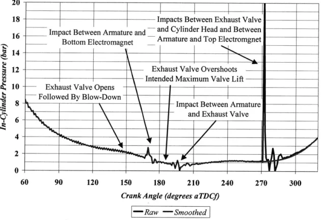
The exhaust manifold system consisted of a relatively short 38 mm diameter pipe connecting the exhaust port to the exhaust trench. An ETAS sensor which reported the fuel-air equivalence ratio of the exhaust gas was located just downstream of the exhaust port. A typical plot of in-cylinder pressure during the exhaust event is depicted in Figure 2.7. It is obvious that the in-cylinder pressure is affected by flow dynamics in the exhaust port and manifold as the pressure drops below 1 (bar) about bottom-dead-center (BDC) then briefly goes above 1 bar before finally settling to 1 bar at EVC. The spikes in pressure are generated by a mechanical impact between the exhaust valve and armature and by impacts between those components and the cylinder head and both electromagnets.

Throughout this study, the in-cylinder work, equal to jpdV, was used to determine

engine output. Note that the spikes in pressure, caused by the aforementioned mechanical impacts of the valve mechanism, can significantly affect the calculation of that quantity. This is especially true about EVC and IVC where the magnitudes of the spikes are greatest and where the change in volume can be quite large. In order to minimize any errors, the in-cylinder pressure was "smoothed" using a 3rd order polynomial about IVC and EVC as depicted in Figure 2.7.

20 18 16 ~14 12 10 8 6 4 2 0 60 90 120 150 180 210 240 270 300

Crank Angle (degrees aTDC) -Raw -Smoothed

Figure 2.7 Typical In-Cylinder Pressure During the Exhaust Event

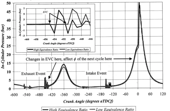
The intake manifold system consisted of a 2 kW air heater to control the intake manifold temperature (IMT) followed by approximately 750 mm of 30 mm diameter pipe leading to the intake port. _{IMT was controlled to either 120 +0/-2 "C or 120 +0/-20 "C with an on/off} controller. Figure 2.8 depicts typical time histories of IMT. There was no throttle plate in the intake manifold. Like the exhaust port and manifold, flow dynamics in the intake port and

Impacts Between Exhaust Valve Impact Between Armature and - and Cylinder Head and Between Bottom Electromagnet _Armature and Top Electromgnet

Exhaust Valve Overshoots _

Intended Maximum Valve Lift Exhaust Valve Opens

Followed By BlowDown

-Impact Between Armature and Exhaust Valve

manifold affect the in-cylinder pressure during the intake event as depicted in Figure 2.9. Again, the spikes in pressure are caused by mechanical impacts between the valve, armature, cylinder head and both electromagnets. An Omega PX176-025A5V pressure transducer was used to measure the manifold absolute pressure (MAP). The in-cylinder pressure was then pegged by minimizing the error between it and MAP in the region between 525 and 5402 degrees aTDCf.

I.. I.. 122 120 118 116 114 112 110 108 106 104 102 100 98 0 100 200 300 400 500 Engine Cycle 600 700 800 900 1000 120 +01-2 degrees C -120 +0/-20 degrees C

Figure 2.8 Typical Time Histories of IMT

2 Since the intake valve was allowed to close as early as 540 degrees, it was impossible to peg the in-cylinder

pressure to angles greater than that without introducing errors caused by the pressure spikes.

-O ---

-1.5 1.4 1.3 1.2 1.1 1 0.9 0.8 0.7 0.6 fig 390 420 450 480 510 540 570 600 630

Crank Angle (degrees aTD C)

-In-Cylinder Pressure -Intake Manifold Pressure

Figure 2.9 Typical In-Cylinder Pressure During the Intake Event

2.2.5 Fuel Injection System

A pulse actuated solenoid fuel injector was located just upstream of the intake port and

oriented so that the fuel spray was directed toward the port walls and the backside of the intake valve. To avoid erroneous temperature measurements due to evaporation of various quantities of fuel, the thermocouple used to monitor IMT was located just upstream of the injector. An electric fuel pump and pressure regulator maintained a constant difference in pressure equal to 2.7 bar between the fuel line and the intake manifold. Calibration measurements of the fuel injection system showed that the mass of fuel injected into the port per cycle was a linear function of the duration of the electronic pulse used to activate the solenoid injector. The relationship between mass of fuel injected per cycle and injector pulse width is depicted Figure 2.10. The expression relating mass of fuel to the injection duration is given by:

Intake Valve Opens _ Intake Valve Closes

-In-Cylinder Pressure

Mfue,(mg)= 2.2783 1000 (deg)-0.5732 6rpm 50 45 40 35 30 25 20 15 10 5 0 (1) 0 2 4 6 8 10 12 14 16 18 20 Pulse Width (ms)

Figure 2.10 Relationship Between Mass of Fuel Injected and Injector Pulse Width

The fuel used in this study was Chevron-Phillips UTG-91. See Appendix A. By weight, this fuel consists of 86.36% Carbon (C) and 13.41% Hydrogen (H) giving a chemical formula of

CH 1.8 53. Chevron-Phillips estimated its molecular weight to be 107 gm/mol. Furthermore, it

was assumed that any HC molecules in the exhaust took the form of CH1.85 and that the

thermodynamic properties of the HC were approximately equal to those of methylene (CH2).

2.3

Controller Software and Electronics

The stated objective of this study was to develop an engine controller capable of maintaining a constant fuel-air equivalence ratio while simultaneously managing load transitions

y=2.2783x - 0.5732

R 2 = 0.9999 00

'000--within the CAI operating regime. It will be shown in Chapter 4: SYSTEM

IDENTIFICATION OF THE CAI ENGINE that combustion in the CAI regime depends

almost entirely on in-cylinder conditions created by the inputs to the engine during the previous cycle. As such, the engine controller must be capable of true cycle-by-cycle control. That means the controller must be capable of assessing the output of the previous engine cycle, using that assessment to determine the inputs required in the current engine cycle and actuating those inputs in a timely manner. In addition, the controller must be capable of sending and receiving information to and from the engine operator so that the operator can both command a desired output and monitor the engine's ability to produce that output. If the controller fails to achieve any of these goals the CAI engine may run poorly or not all. It is not difficult to imagine the detrimental effects that incorrect fuel quantity or valve timings would have on the performance of the CAI engine. Worse, failure of the engine controller to perform as expected could have catastrophic results if the piston were to strike an unclosed valve or if an open fuel injector were to flood the engine cylinder leading to hydraulic lock or an explosion.

2.3.1 Data Acquisition System

After careful consideration of the engine controller's importance to this study, National Instruments Lab View 7.0 software running in real-time on a NI PXI-1042 chassis was selected as the platform upon which the controller was to be built. Two National Instruments PXI-6070E Multifunction

I/O

Litton 70HDIN360-1-2-0 encoder with one-degree crank angle resolution was used to determine engine position. Note that the resolution of the encoder is significant because it effectively determined the resolution of the input actuation signals. In this study, those signals were constrained to start and end on integral multiples of crank angle.

2.3.2 Engine Controller Logic

Figure 2.11 shows the typical timing of the input events in an engine cycle; i.e. -360 to

360 degrees aTDCf. The events are exhaust valve closing (EVC) and, by symmetry, intake valve

opening (IVO), intake valve closing (IVC) and fuel injection3 _{to the engine when operating in}

CAI mode. There are times in the CAI engine cycle during which the valves must be open, the spark plug must be energized4 _{and the fuel injector must be injecting fuel. The solid lines}

indicate those times in Figure 2.11. Conversely, since there is flexibility in the duration of the valve events and the mass of fuel to be injected, there are times in the engine cycle during which the valves may or may not be open and when the fuel injector may or may not be injecting fuel. The dashed lines depict those indeterminate times. Finally, mechanical considerations; i.e. inertia and friction, introduce a delay of approximately 4-5 ms (45 degrees at 1500 rpm) between when the boost current is turned on, denoted by the arrowheads, and when the valve actually opens. The arrows are included on the figure to highlight the fact that the controller is actively controlling the intake and exhaust valves before those valves even open.

3 In this study, exhaust valve opening was fixed at 150 degrees aTDCf.

4 Although a spark is not required in CAI mode, its use is a convenient and easy method of avoiding misfire. In this study, the spark was set to TDCf under all conditions.

Intak (Open

w

3

I

Exhaust Bottom Magnet (Open) Boost Current On e Bottom Magnet Boost Current On Minimum Intake Duration Range of IVC Spark End/Start ofC ange of IVO I I - 1 14 I I I I I I I -360 -300 -240 -180 -120 -60 0 60 120 180 240 300 360

Crank Angle (degrees aTDCf)

Figure 2.11 Valve, Spark and Fuel Injection Events

A typical CAI combustion event occurs just after TDCf. Since this event is driven by

chemical kinetics and not by an external ignition source, it is reasonable to infer that combustion in any given cycle is dependent on combustion in the preceding cycle and any input to the engine that occurred during that cycle. Since the controller is responsible for all input to the engine, it seems logical that the controller cycle encompass all input between any two combustion events. The value of 5 degrees aTDCf was chosen as the end and start of the controller cycle because it strikes a good balance between maximizing the residence time of exhaust gas at the exhaust gas fuel-air equivalence ratio sensor and allowing the controller sufficient time to communicate with the engine operator, read in the cylinder pressure, engine speed, MAP and

#

I I Fuel Minimum Fuel . Injection Duration EVO Minimum

Exhaust Duration _{Range of EVC}

ontroller Cycle R

controller cycle. In this mode, the controller is focused solely on actuating the inputs and cannot be interrupted. If it were to be interrupted, it might miss a valve, spark or fuel event and thereby adversely affect engine performance or worse. A flowchart of the engine controller is depicted in Figure 2.12.

START

Wait for TDC Marker

*

Communicate With Engine Operator

Read All Data From Previous Cycle

Calculate Input

Advance 1 Crank Determine Current

Angle Crank Angle

NO

Time for Fuel, Valve or YES Is Crank Angle < 725

1

Spark Event? Degrees aTDCf?

YES NO

Turn On/Off 5 Volt _{Turn Controller Off?} Digital Signals

r YES

I END

4-AL

Figure 2.12 Flowchart of the Engine Controller A

2.3.3 Additional Engine Controller Electronics

The 5 Volt digital output signals referred to above were sufficient to actuate the spark and fuel injection systems but were not sufficient to actuate the VVT system. Recall that the electromagnets are subject to both a hold current and a boost current that differ by an order of magnitude. Since the controller is only capable of outputting 5 Volt digital signals, an additional electronic circuit between the PXI controller and the Brush Type PWM Servo Amplifiers was required. This circuit consisted of four operational amplifiers acting as voltage summers. The input to each summer were two 5 Volt digital signals; one to turn on and turn off the boost current and one to turn on and turn off the hold current. A schematic of one of the circuits is depicted in Figure 2.13. Note that once the input and output resistances of the voltage summer were chosen, the boost and hold voltages were fixed. The selection of those resistances is not critical to the control of the CAI engine and thus will not be discussed here.

Rsum,inverse >oost Rnverse 5V TTL, boost Wnerse 5V TTL, hold

I

Figure 2.13 Intermediate VVT System Circuitry

2.3.4 Engine Controller Program

As stated previously, the engine controller was developed using LabView 7.0 real-time software. The program consists of nearly 100 interconnected subroutines or sub-Vis.

Chapter 3: Open-Loop Control of the CAI Engine

3.1 Introduction

The simplest means of controlling the CAI/SI engine operating in CAI model is by open-loop control as illustrated in Figure 3.1. In this mode of control, the operator commands a desired engine output (d); i.e. the desired in-cylinder mean effective pressure (MEP)2 and exhaust gas fuel-air equivalence ratio (0). The desired outputs are, in turn, used to determine the required input to the engine (u); i.e. the fuel injection duration (Ofuel), the angle at which the intake valve closes (IVC) and the angle at which the exhaust valve closes (EVC), that will produce that output. Note that for this method of control, the CAI engine is effectively a black box in that no information beyond a predetermined input/output relationship is known. There is also no output feedback and thus no way to insure that the actual engine output (y) is, in fact, equal to that which is desired. Given that the output of the CAI engine is a strong function of the engine's environment; i.e. intake manifold temperature (IMT), engine coolant temperature, fuel composition and manifolding, and operating conditions; i.e. engine speed, the open-loop controller should be a poor choice of control for the CAI engine. Nonetheless, it is appropriate to describe the open-loop controller since its development was an important milestone in both the system identification process to be described in Chapter 4: System Identification of the CAI

1 Heretofore, the CAI/SI engine operating in CAI mode will be referred to as the CAI engine.

fPdV

2 Strictly speaking, the quantity by _this definition, _{is not equal to NIMEP since the cycle over which the}

Vd

pressure is integrated (from -30 degrees aTDCf over 720 degrees) does not correspond to the traditional definition of an engine cycle (integration from -360 degrees aTDCf over 720 degrees). This point will be discussed in

4PdV

significant detail in Chapter 4. For now, it is sufficient to note that the quantity will be referred to as MEP

Vd

Engine and the development of the closed-loop controller to be described in Chapter 5: Model

Development and Closed-Loop Control of the CAT Engine.

d Mapping UEgn

of dto u

Figure 3.1 Schematic of Open-Loop Controller

3.2 Mapping of Input versus Output

The required inputs are said to be "mapped" functions of the desired outputs. For the

CAI engine operating at a particular engine speed, IMT and engine coolant temperature, the

mapping of required input versus desired output for a given cycle i, took the form of:

ui = Md.1 +c, ₍₁₎

where u is the [3x1] vector of required input, d+1 is the [2x1]vector of desired output, M is a [3x2] matrix of constants and cu is a [3xl] vector of constants. The subscripts i and i+1 reference a particular engine cycle as depicted in Figure 3.2. Note that the inputs u are imposed on the engine during cycle i but that the outputs y, correspond to the cycle in which they are calculated, not the cycle in which they are produced. For example, in Figure 3.2, the quantity

PdV

is denoted MEP+1 since it cannot be calculated until cycle i has ended and cycle i+1 has VA

control, they were defined in this way to faciliate the construction of the closed-loop controller as will become apparent in Chapter 5.

45 40 35 30 25 20 15 10 5 0 -360 -270 -180 -90 0 90 180 360/-360 -180 -90

Cra nk Angle (degrees a TD CQ)

corresponds to start of CAI cycle i+1 (-30" aTDCf)

Figure 3.2 CAI Cycles Defined

0 90 180 270

3.2.1 Experimental Data

In order to determine the matrices M and c., the CAI engine was run with nine distinct combinations of input. The inputs were chosen such that the engine output would span the range of feasible MEP at 1500 rpm; i.e. approximately 3.25 bar as limited by combustion instability to approximately 4.75 bar as limited by engine knock. The engine was run with stoichiometric (4

=1), lean (4<1) and rich ( >I) exhaust gas fuel-air equivalence ratios. Since the input is not

continuous, but rather constrained to integer multiples of one crank angle degree, it was

impossible to achieve the exact same value of MEP at each of the three values of

#.

- - CAI cycle i K

CAI cycle i-1 -- - CAI cycle i+1

combustion

controller cycle i/i+1 end/start (50aTDCf)

calculate y j.;, x ., u

-start of CAI cycle

-CAI cycle /1+1 end/start (-30' aTDCf)

0

fuels

EVO, EVC, IVO, IVC,

_T_ __ _

41 1

I

* x+1t

impossible to achieve the exact same values of

#.

#,

produced minimal knock at high values of MEP and acceptable combustion stability at low values of MEP. There was no effort made to optimize fuel consumption or to minimize emissions. Table 3.1 summarizes the nine combinations of MEP and

#

#

#

3.1 are equal to the average output of the CAI engine over 1000 cycles. Figure 3.3 depicts the

time-history of MEP for a stoichiometric equivalence ratio. Close inspection of Figure 3.3 reveals an increase in the cycle-to-cycle variability of MEP as the mean value increases. Since there is no feedback, this cycle-to-cycle variability is of little interest when discussing open loop control of the CAI engine. However, when considering feedback or closed-loop control, cycle-to-cycle variability can be extremely important. Figure 3.4 depicts the time-history of

#

#,

Table 3.1 Mean Values of MEP and 0 versus Ofue, IVC and EVC

NIMEP (bar 4.76 4.79 4.49 4.09 4.08 3.97 3.33 3.38 3.37 1.03 1.00 0.96 1.03 1.00 .95 1.03 0.99 0.95

Oruel 69 66 63 60 59 57 52 51 50

IVC (deg) 567 570 573 561 564 564 555 557 557

II

I

$AULuMm!AMt

- - I I I I I I I I

-100 200 300 400 500 600 700 800 900 1000

Engine Cycle

-Max MEP, phi = 1 -Mid MEP, phi = 1 -- Min MEP, phi = 1

Figure 3.3 Typical Cycle-to-Cycle Values of MEP for Constant Input

1 nQ 1.06 1.04 -1.02 .

1

-Median MEP, phi > 1 -Median MEP, phi = 1 -m-Median MEP, phi < 1

Figure 3.4 Typical Cycle-to-Cycle Values of

#

5 4.75 4.5 4.25 34 S3.5 3.25 3 -0 I1 I .2