HAL Id: hal-00948017
https://hal.archives-ouvertes.fr/hal-00948017
Submitted on 17 Feb 2014HAL is a multi-disciplinary open access archive for the deposit and dissemination of sci-entific research documents, whether they are pub-lished or not. The documents may come from teaching and research institutions in France or abroad, or from public or private research centers.
L’archive ouverte pluridisciplinaire HAL, est destinée au dépôt et à la diffusion de documents scientifiques de niveau recherche, publiés ou non, émanant des établissements d’enseignement et de recherche français ou étrangers, des laboratoires publics ou privés.
Fuzzy controller tuning of a boost rectifier unity power
factor correction by experimental designs
Jérôme Faucher, Stéphane Caux, Pascal Maussion
To cite this version:
Jérôme Faucher, Stéphane Caux, Pascal Maussion. Fuzzy controller tuning of a boost rectifier unity power factor correction by experimental designs. Electrical Engineering, Springer Verlag, 2009, vol. 91, pp. 167-176. �10.1007/s00202-009-0131-0�. �hal-00948017�
O
pen
A
rchive
T
OULOUSE
A
rchive
O
uverte (
OATAO
)
OATAO is an open access repository that collects the work of Toulouse researchers and
makes it freely available over the web where possible.
This is an author-deposited version published in :
http://oatao.univ-toulouse.fr/
Eprints ID : 10971
To link to this article : DOI: 10.1007/s00202-009-0131-0
http://dx.doi.org/10.1007/s00202-009-0131-0
To cite this version Faucher, Jérôme and Caux, Stéphane and
Maussion, Pascal Fuzzy controller tuning of a boost rectifier unity
power factor correction by experimental designs. (2009) Electrical
Engineering (Archiv fur Elektrotechnik), vol. 91 (n° 3). pp. 167-176.
ISSN 0948-7921
Any correspondance concerning this service should be sent to the repository
administrator:
[email protected]
FUZZY CONTROLLER TUNING OF A BOOST RECTIFIER UNITY POWER
FACTOR CORRECTION BY EXPERIMENTAL DESIGNS
!
J.D. Faucher
12, S. Caux
12and P. Maussion
12 1Université de Toulouse ; INPT, UPS ; LAPLACE (Laboratoire Plasma et Conversion d’Energie) ; ENSEEIHT, 2 rue Charles Camichel, BP 7122, F-31071 Toulouse cedex 7, France.
2
CNRS ; LAPLACE ; F-31071 Toulouse, France.
!
Abstract: This paper shows the validity of experimental designs as an efficient on-site tuning tool for fuzzy controllers, dedicated to electrical engineering applications with multi-objective criteria. Our purpose is to improve the input and output system characteristics that is to say the global quality of the electrical power in a boost rectifier with unity power factor correction. The desirability notion combines here time dynamic and harmonic criteria, it illustrates the trade-off that has to be satisfied between the different properties.
!
Keywords: fuzzy control, experimental designs, tuning methodology, multi-objective criterion, boost rectifier, power factor correction, desirability.
1. INTRODUCTION !
Our work deals with the tuning of fuzzy controller in order to improve the control of electric systems. Fuzzy-logic-based controllers are used in various applications, mainly because of advantages such as the dynamic performance, the robustness or the possibility to take into account an experimental knowledge of the process.
Nevertheless, some drawbacks have to be underlined: first, the huge number of parameters that have to be tuned even for a very simple fuzzy structure and the lack of an efficient on-site tuning strategy for all these parameters. The fuzzy controller parameters could of course be tuned trough trial-and-error procedure, but it could be quite long and rather delicate. On the other hand, some methods have already been proposed, for the tuning of fuzzy controllers, using adaptive algorithms (Barrero, 1995) and (Kang et al, 1992), additional fuzzy rules (Takagi, 1992), neural networks (Perneel et al, 1995), H! and LMI methods (Liu et al, 2001) and (Park, 2004) or genetic algorithms
(Hoffmann, 2001). These tuning methods are successful but are generally far from simple.
Besides, a simple tuning methodology based upon experimental on-line designs for all the parameters of a PID-like-fuzzy-logic controller have already been proposed (Hissel et al., 1999) few years ago. This method, based on time criterion only, for fuzzy controller tuning gave experimental and simple pre-established settings just like the well-known Ziegler-Nichols methods for the classical PID controllers.
Our aim is now to show that experimental designs methodology could be an efficient tool in order to tune fuzzy controllers for applications that require multi-objective criteria. In this paper, the methodology will be applied to a single phase boost rectifier with unity power factor correction. This kind of converter is strongly nonlinear, it means that linear controllers are not truly efficient, especially when sudden and hard parameter variations due to high load variations occur. Then a fuzzy controller should be an efficient solution for the control of such a converter. Two criteria have to be regarded: a time-response-based criterion on the output voltage and an harmonic criterion based on the input current distortion on the grid. Fuzzy controllers have already been used for this system control (Yu et al. 1996), (Henry et al., 1999), (Pires et al., 1999) and (Mattavelli et al., 1995), and the harmonic reduction by fuzzy control has been shown in (Palandöken, 2003) but there is still a lack of efficient tuning methodology. This paper will show how the experimental designs could be an efficient tool, in simulation or on the experimental process, for the on-site tuning of a nonlinear controller under those specifics constraints. This is the main contribution of our work.
Section 2 describes the system and its classical linear control is presented in section 3. The structure of the fuzzy controller is given by section 4 while section 5 describes the experimental design methodology, applied in section 6 for the tuning of the fuzzy controller. Simulation results are presented in section 7, experimental results in section 8 and their comparison in section 9. Finally, section 10 concludes the paper and gives some trends for future works.
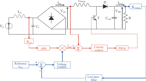
2. SYSTEM DESCRIPTION
2.1 System description
The system is a single phase boost rectifier with unity power factor correction and 1kW nominal power. In a classical solution with a diode bridge rectifier, an additional capacitor reduces the voltage ripple. However, this capacitor also reduces the diode conduction angles and generates harmonic distortion on the electrical network described by Vn (network voltage) and Ln (network inductance). In order to solve theses problems, a boost converter is added to the
system. The capacitor Cout is the output filter for the load that needs a constant voltage. The values of these different components are given in table 1.
Fig. 1. System structure
Vn 325V Rload 100 Ln 0.1 mH R0 2000 Cf 25 !F Kvmeas 1/100
Lboost 4 mH Kvn 1/325
Cout 500 !F Ref VDC 4 V Tab. 1. System parameters values
Hard and sudden load variations are applied to the system in order to evaluate the performance of the control strategy. The benchmark test is the following: from steady-state operation under no load conditions (R = R0) to sudden maximum load connection (R=Rload), and sudden disconnection. In addition, it is important to notice that capacitor Cf prevents high frequency harmonics from going back to the network. A cut-off frequency Fc chosen above the higher frequency (the 100 Hz frequency of the rectified voltage Vrec) and around one decade below the switching frequency (20 kHz) is suitable. We fix Cf = 25 !F , that means Fc = 500 Hz (1).
f f c C L F . 2 1
"
# (1)A complementary study shows that this Cf value also reduces the current distortion under no load conditions.
2.2 Behaviour requirement
The boost rectifier has some characteristics that impose a constraint on the output voltage. When transistor T is ON, the diode D is OFF (VD = - VDC) and :
0
$
#
boost rec recL
V
dt
dI
(2)When transistor T is OFF, the diode D is ON (ID = Irec) and :
0
$
%
#
boost DC rec recL
V
V
dt
dI
(3)Thus, whatever the state of the transistor, while
&
,
$
0
dt
dI
V
V
recrec
DC . In such a configuration, the system is not controllable until
V
DC#
V
rec. In conclusion, this system requires thatV
DC$
V
rec, that is why it is called “boost”.Cf Lboost D T Cout R Vn Ln ABS + -Current control PWM Voltage Control + Reference VDC Low pass filter Vrec VDC Kvn Kvmeas
-Iref Irec Iloadt VDC IAE THD Load No load 3. LINEAR CONTROL
The control of this kind of system is usually done by linear controllers. Performance of such controllers will be the reference for a comparison with the fuzzy controllers and also their initial parameter values. There are two control loops (figure 1), one for the dc output voltage and the other for the rectified input current.
3.1 Current loop
The objective of this “fast” loop is to get a sinusoidal current in phase with the electrical grid voltage. Thus, it reduces the harmonic rejection and maintains a unity power factor. A linear PI controller is used in combination with a PWM module. The high frequency harmonics are then reduced with this kind of control. The shape of the current reference is generated from the network voltage (via Kvn) and its amplitude from the DC voltage (via the voltage controller) as shown in figure 1. The transfer function of the PI current controller is:
ic ic c current
T
p
T
p
G
p
H
.
)
.
1
(
.
)
(
#
'
(4) and s3 + 1.75 (n s2 + 3.25 s (n2 + (n3 (5)The PI controller is tuned according to (Dorf, 1990), in order to make the denominator of the current closed loop transfer function fit a specific equation (5) that minimizes the ITAE criterion. These considerations lead to the following coefficients (6) :
Gc = 2.1 and Tic = 0,28 ms (6)
Figure 2 shows the simulation results with the PI controller. One can check the efficiency since the rectified current is closed to its reference and contains very few low frequency harmonics.
Fig. 2. Current control: Irec and Iref Fig. 3. Criterion measurement and benchmark test.
3.2 Voltage loop
This “slow” loop must control the output voltage VDC with respect to load, input voltage and input current variations. A classical PI controller tuning is based on the average model of the system. This method relies on the equilibrium of the instantaneous powers between the output of the rectifier and the DC part (Yu, 1996). If the current loop is fast enough compared to the voltage loop, approximation (7) could be done, and the transfer function is given by (8).
) ( ) ( ) ( ) ( p I p V p I p V ref DC rec DC ) (7) 2 . . 1 . . 4 ) ( out load load rec ref DC C R p R V V I p V ' # (8)
where
V
is the VDC average value. As the transfer function of the voltage controller is given by equation (9), optimum symmetrical methodology leads to the following coefficients (10).iv iv v voltage
T
p
T
p
G
p
H
.
)
.
1
(
.
)
(
#
'
(9) * + , # # 062 . 0 5 . 7 iv v T G (10)Control action Normalisation em 1 dem 1 gm Denormalisation Integral action Fuzzy controller Spi e de
3.3 Different tuning criteria
The control quality for the whole system will be evaluated trough two criteria. The first one is the IAE (integral of absolute error, expression (11). This criterion applied to VDC will show the robustness and the dynamic performance of the controller. In addition, a second criterion, the harmonic distortion rate (THD) in (12), represents the harmonic rejection quality at the input.
dt
t
e
IAE
#
-
(
)
.
(11).
100
39 1 39 2 %.
.
# ##
k k k kI
I
THD
(12)The CEI 61000-3-2 international standard defines the electromagnetic compatibility and limits the harmonic current emissions for the 39 first harmonics. It gives the maximum allowable current amplitude for each harmonic. Figure 3 shows how and when the two different criteria are calculated during the benchmark test. The IAE criterion is taken into account throughout the test. The harmonic distortion is only computed during steady-state operation under rated load condition, i.e. rated current.
4. FUZZY CONTROLLER
A fuzzy controller will be used in the rest of this paper in order to improve the dynamic performance. The controller is a PI-like fuzzy controller (FLC) (see figure 4). This structure was chosen because the error’s second derivative does not have to be calculated. Indeed, its value could be important as it may amplify noise. The inherent difficulty of such a kind of controller is the huge number of parameters. The fuzzy part consists into two inputs / one output Sugeno FLC (Hissel et al. 1999) with seven triangular membership functions on each input and seven singletons at the output. There is a normalisation factor for each input (em for the error signal and dem for the error derivative) and for the output (gm).
Experiment number Factor 1 Factor 2 Interaction 12 Criterion 1 - - + y1 2 + - - y2 3 - + - y3 4 + + + y4 Effects E1 E2 E12
Fig. 4. Fuzzy controller structure. Fig 5 : Example of an experimental table
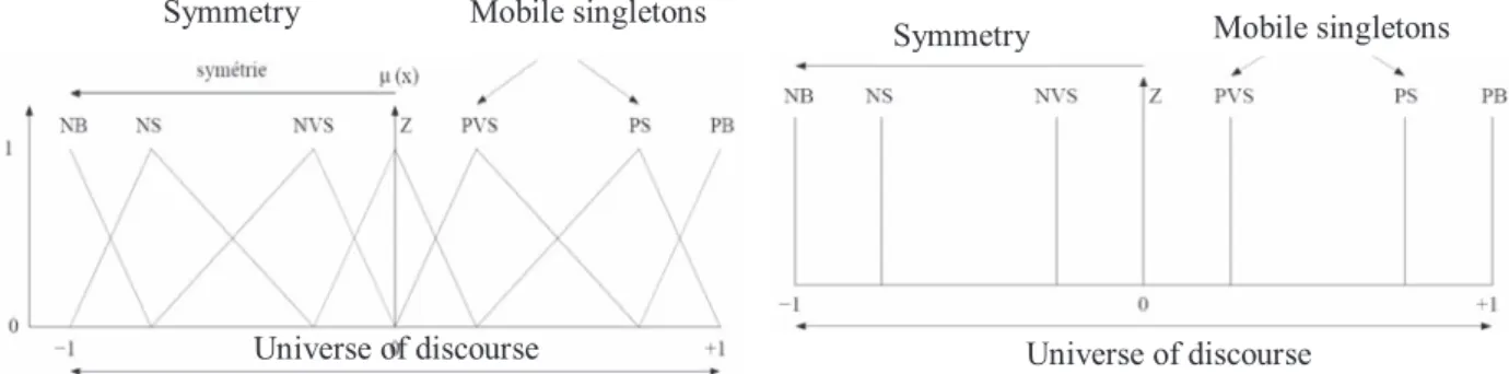
A zero-symmetry is imposed for both triangular membership functions and singletons in order to provide a similar response for positive and negative inputs. A classical anti-diagonal rule table, with fixed parameters, is used. By fixing em to the reference value, only 8 parameters have to be tuned among the initial 73 ones (7*7 rules, 3*7 membership functions and 3 gains). The tuning parameters are: dem, gm, PSe and PVSe (membership functions on error), PSde and PVSde (membership functions on error derivative), given by figure 6 and PSs and PVSs (output singletons), given by figure 7. For example, PSe is the label of the Positive Small membership function on the error and PVSde is the label of the Positive Small membership function on the derivative of the error. The positions of these membership functions have to be tuned. Anyway, the tuning problem remains effective as 8 control parameters are to be tuned according to two criteria.
Fig. 6. Membership functions for error and derivative of error inputs
Fig. 7 : Output singletons Mobile singletons Symmetry Universe of discourse Mobile singletons Universe of discourse Symmetry
Fuzzy logic is only used for the PI like controller on the voltage loop. Due to frequency limitation of our DSP, the current loop must be continuous (the sampling period is Te#1.10%4s ). Moreover, two fuzzy controllers for the same system would dramatically increase the number of parameters that have to be tuned.
5. EXPERIMENTAL DESIGNS PRINCIPLES
The history of experimental designs began in the 30’s in England with M. Fisher, (Fisher, 1935) but it had an increasing development since Taguchi published predefined tables (Taguchi, 1987). This methodology realizes a schedule of the experiments in order to obtain the most accurate information for a specific problem with a minimum number of experiments (Dey et al., 1999). The idea is to modify the level of each factor for each experiment according to a specific procedure. It allows a drastic reduction of the number of experiments, an increase in the number of parameters, the detection of interactions between factors and gives an optimized solution.
Considering for example only two levels for each of the 8 factors described above, the classical experimental tuning method that consists in varying one of the parameters when all the others are maintained constant, leads to 28=256 required experiments. With experimental designs methodology, only 16 experiments out of 256 are necessary to find the suitable combination for the 8 factor levels in order to minimize the selected criterion
We use centred reduced variables, i.e. -1 for the low level and +1 for the high level of each factor. Then, an experimental table, as shown in figure 5, could be used. Each line represents an experiment and each column is a factor, an input MF, an output singleton position or a gain. For each experiment, the criterion is calculated through simulation or measured during experiments.
4 4 3 2 1 1 y y y y E # % ' % ' (13) 4 4 3 2 1 12 y y y y E # % % ' (14) According to the experimental design methodology (Dey et al., 1999), the effect of a factor is obtained through equation (13). For example, E1 = 0.12 means that factor 1 at high level has an effect of +0.12 on the criterion. Moreover, the effect of interactions between factors can also be investigated with this methodology. Expression (14) leads to the effect of interaction E12 between factor 1 and 2, on the desired criterion. Furthermore, the same column could also be used to study a third factor. From these effects, an optimal tuning could be reached, with a last experiment in order to confirm the design. If the results are irrelevant, then the hypotheses must be reconsidered.
The experiment table is built like an Hadamard matrix (Droesbeke, 1997) that verifies equation (15), where n is the number of experiments. Such a structure gives the best accuracy on effects. Indeed, the standard deviation on the effect ( E ) is a fraction of the standard deviation on the criterion ( y ), as shown in equation (16) :
nI X t X . # (15)
n
y E/
/ #
(16) 2 1 _ , 21
1
.
#0
1
2
3
4
5
%
%
#
N j i j i iy
y
N
s
(17)A major problem is the determination of the experimental error. The accuracy of the estimation s, the experimental standard deviation on the criterion y, depends on the number of experiments. By repeating N times each experiment of the design table, the estimation si for each experiment is improved. yi,j is the jth repetition of the ith experiment and
_
i
y is
the average of the N repetitions of the ith experiment. The variance is given by equation (17). The classical isovariance assumption is considered and equation (18) can be written. Afterwards the estimation of the experimental standard deviation on the effect, sE, is expressed in (19).
n s s s n i i i
.
# # # 1 2 _ 2 (18)n
N
s
s
E.
#
(19)The confidence interval is thus balanced by the variable of Student
t
6n.(N%1) at n.(N-1) degrees of freedom with the probability " to be exceeded in absolute value. As a consequence the confidence interval for a probability " isE N n
s
t
7
8
.( % )16 around the average effect value.
6. TUNING METHODOLOGY
6.1 Parameter values
In this controller, 8 parameters have to be tuned. The initial levels of parameters are always difficult to choose, an accurate expertise on the system is required. The values of the continuous PI controller parameters will be used as
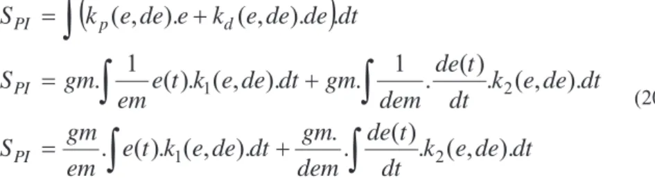
initial values. Regarding SPI as the fuzzy controller output, on figure 4, equation 20 can be defined. kp is the proportional gain and kd is the derivative one of the first part of the fuzzy controller.
9
:
dt
de
e
k
dt
t
de
dem
gm
dt
de
e
k
t
e
em
gm
S
dt
de
e
k
dt
t
de
dem
gm
dt
de
e
k
t
e
em
gm
S
dt
de
de
e
k
e
de
e
k
S
PI PI d p PI).
,
(
.
)
(
.
.
).
,
(
.
)
(
.
).
,
(
.
)
(
.
1
.
).
,
(
.
)
(
1
.
.
).
,
(
).
,
(
2 1 2 1-'
#
'
#
'
#
(20)Then, equation 20 reveals two different actions: integral and proportional of the complete PI-like-fuzzy controller which can be used for initial tuning. If the error is sampled at the sampling period Te, expressions (21) can be written, and from the transfer function Hvoltage, it comes (22) :
;* ; + , % % < < Te k e k e t de k e t e ) 1 ( ) ( ) ( ) ( ) ( (21) ; ; * ;; + , # # v iv v G dem Te gm T G em gm . (22)
The levels of the membership functions are chosen on both sides of the values of the equi-distributed membership function positions. Similar choices are made for gm and dem coefficients.
6.2. Experimental table
As there are 8 parameters, a 28-4IV Hadamard experimental table is used, which implies only 16 experiments. Table 2 presents the experimental designs table.
exp F1 PSe F2 PVSe F3 PSde F 4 PVSde F5=234 and PSs F 6=134 and PVSs F7=123 and gm F 8=124 and dem 1 - - - - 2 + - - - - + + + 3 - + - - + - + + 4 + + - - + + - - 5 - - + - + + + - 6 + - + - + - - + 7 - + + - - + - + 8 + + + - - - + - 9 - - - + + + - + 10 + - - + + - + - 11 - + - + - + + - 12 + + - + - - - + 13 - - + + - - + + 14 + - + + - + - - 15 - + + + + - - - 16 + + + + + + + +
Tab. 2. First set of factors levels in a 28-4IV experimental table
The two criteria (IAE and THD) are calculated during simulations or measured during the experiments. It is important to notice that each experiment is run once in simulation but has to be repeated during experimental tests, in order to reduce the experimental standard deviation on the effect, as seen in section 5.
6.3 Desirability
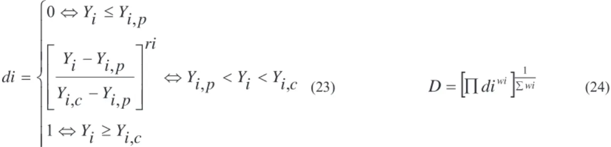
The desirability notion was introduced by E.C. Harrington (Harrington, 1965). It combines several different properties Yi with different scales and units (Derringer et al. 1994). Each of them is transformed in an elementary desirability function di, as seen in equation (23). A desirability function is ranged between zero and one.
A zero level corresponds to an unacceptable value for the criterion while a desirability of one represents the maximum desired performance. Many different transformations could be chosen. The most classical one was adopted due to its simplicity, it is described below. The value of Yi,p is the minimum acceptable value for Yi and Yi,c is the value above whom an amelioration of Yi is not very interesting.
;
;
;
*
;
;
;
+
,
=
=
>
?
@
@
A
B
C
D
&
&
D
%
%
E
D
#
c
i
Y
i
Y
c
i
Y
i
Y
p
i
Y
ri
p
i
Y
c
i
Y
p
i
Y
i
Y
p
i
Y
i
Y
di
,
1
,
,
,
,
,
,
0
(23)D
#
F
H
di
wiG
.wi 1 (24)The parameters ri balance the importance of the increase of the property on the elementary desirability (Fig. 7). Then, all the elementary desirabilities are combined into a composite desirability such as in equation (24) :
0 0.5 1 1.5 2 2.5 3 3.5 4 4.5 300 320 340 360 380 400 420 440 460 480 500 520 Time (s) V o lt a g e ( V ) Analogical PI Fuzzy PI
Fig.8 Elementary desirability Fig.9Simulated output voltage responses
7. SIMULATION RESULTS
Two successive designs are carried out in simulation using desirability in order to combine the dynamic and the harmonic criteria. The first one is a global and “rough” design which gives significant levels for the tuning parameters, the second one improves the tuning. The experimental design, described in table 2 gives then interesting results. 0 0.5 1 1.5 2 2.5 3 3.5 4 4.5 300 320 340 360 380 400 420 440 460 480 500 Time (s) V o lt a g e ( V ) Experimental results Linear PI Fuzzy PI 2.265 2.27 2.275 2.28 2.285 2.29 2.295 -10 -5 0 5 10 C u rr e n t (A ) Irec Inet
Fig.10 Experimental output voltage responses Fig.11 Input currents with fuzzy control
Figure 9 shows the simulation results for the fuzzy controller and the continuous PI. Giving parameter levels, this tuning, set0, is tested also on the experimental process, leading to experimental output responses, figure 10 and 11. Dynamic performance with the fuzzy controller is improved and the harmonic distortion remains low, cf table 8. Only 2 sets of 16 experiments are necessary during this optimization procedure based on the model of the system. But it can be seen that there are some important differences between simulation and experimental results for a single set of parameters (oscillations remains during steady state and the overshoot with experimental fuzzy PI controller is not negligible).
In fact, the model of the system which was used for the simulations tests was not a very fine model and some additional components should be added in order to improve it. But there is another way to improve performance: an
Yi,p Yi,c di Yi ri < 1 ri = 1 ri > 1
on-site and experimental tuning of the controller on the system itself, according to experimental designs methodology. The price to pay is an increased number of experiments in order to improve accuracy.
8. EXPERIMENTAL RESULTS
Instead of system model improvement for a better controller tuning, we applied the experimental designs method directly to the system, with all its characteristics. The whole methodology is detailed hereafter.
8.1 Single criterion
The tuning procedure is then realized on the experimental process. Two successive sets of experiments are again carried out. Parameters of the first “rough” design are given in Tab. 3 from values of the continuous PI controller:
PSe 0.6 PSs 0.6
PVSE 0.3 PVSs 0.3
PSde 0.6 Gm 486
PVSde 0.3 dem 6.5e-3 Tab. 3. Initial fuzzy parameter values
The factor levels are chosen on both sides of initial parameter values:
PSe 0.5 - 0.7 PSs 0.5 - 0.7 PVSe 0.2 – 0.4 PVSs 0.2 – 0.4 PSde 0.5 - 0.7 Gm 490 – 570 PVSde 0.2 – 0.4 dem 5.5e-3 – 7.5e-3
Tab. 4. First set of factor levels.
Considering both criteria in desirability, the experimental design methodology leads to the following set of “roughly optimized” parameters, in Tab.5 :
PSe 0.5 PSs 0.7
PVSE 0.2 PVSs 0.4
PSde 0.7 Gm 530
PVSde 0.2 dem 5.5e-3 Tab. 5. First set of “roughly optimized” parameters
The factor levels for the second and “fine” design are given by Tab. 6 after the first design results.
PSe 0.4 - 0.6 PSs 0.6 - 0.8 PVSe 0.1 – 0.3 PVSs 0.3 - 0.5 PSde 0.6 – 0.8 Gm 490 – 570 PVSde 0.1 – 0.3 dem 45e-4 – 65e-4
Tab. 6. Second set of factors levels.
The two criteria (IAE and THD) are measured for each experiment. The latter is repeated three times for accuracy improvement, (confidence interval defined as 99.9%. Factor effects are given by Table 7. Interaction effects are less influent than main parameter effects and are not given here.
IAE*10-2 V.s TDH*100 % IAE*10-2 V.s TDH*100 % PSe 1.4 -3.1 PSs -2 -3.2 PVSe 3.9 -2.9 PVSs -2.5 8.6 PSde 0.7 -4.3 Gm -2.2 1.5 PVSde 5.6 -21 dem 2.9 -7.2 Average 22.5 364 Confidence interval 0.27 4.04
Tab. 7. Factor effects on both criteria
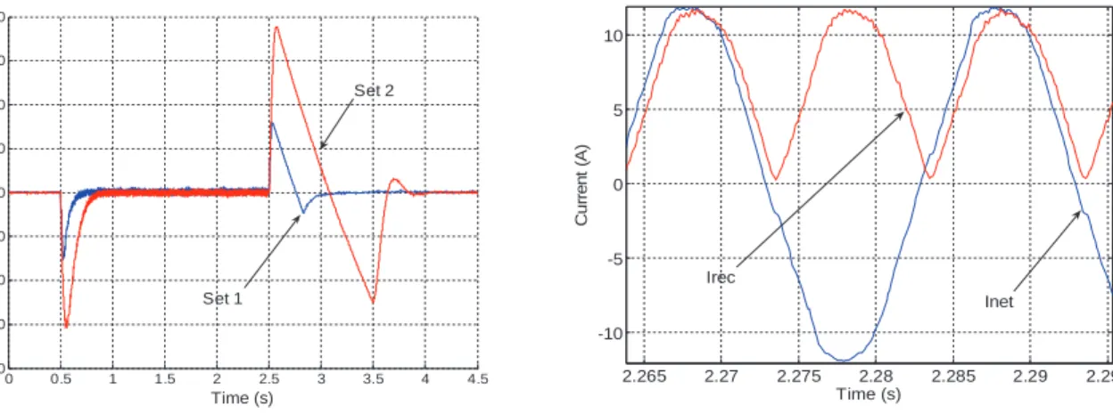
It appears that the factor effects are strongly different for each criterion. The factor PVSde is always the dominant one and its influence is opposite for each criterion, as shown by Table 7. From the factor effects given by the experimental design, a set of optimal parameters for the fuzzy controller can be defined for each criterion: the first one, Set 1, for the IAE criterion only and the second, Set 2, for the harmonic criterion only. Figure 12 presents the
output voltage VDC for the two optimal settings and figure 13 depicts the input current for the second setting only. The criteria values are given in table 8.
0 0.5 1 1.5 2 2.5 3 3.5 4 4.5 320 340 360 380 400 420 440 460 480 Time (s) O u tp u t V o lt a g e ( V ) Set 1 Set 2 2.265 2.27 2.275 2.28 2.285 2.29 2.295 -10 -5 0 5 10 Time (s) C u rr e n t (A ) Irec Inet
Fig. 12. Experimental output voltage responses for set 1 and set 2
Fig. 13. Experimental input currents for Set 2 only
From theses criteria, experimental designs can not give a composite optimal tuning. The solution may consist in a combination of the criteria in a composite criterion with the desirability notion.
8.2 Composite criterion
From the given results, the main difference between harmonic rejection for Set 1 and Set 2 is the value of the third harmonic (0.325 A for Set 1 and 0.113 A for Set 2), the others remaining equivalent. This preponderant harmonic amplitude is then transformed into elementary desirability dh3. Values Yh3,c andYh3,p are equal to Set 1 and Set 2 results with rh3 = 0.1, increasing the penalty for low values. IAE is also transformed into an elementary desirability dIAE, with rIAE = 1and YIAE,c = 0 while YIAE,p is chosen slightly higher than the worst value of the experimental designs. Finally, the harmonic values of the other ranks i are transformed into elementary desirabilities dhi (iJ[2,39],iI3) with Yhi,c = 0 as the objective is to reject harmonic distortion. Yhi,p is equal to the CEI 61000-3-2 standard limit value so as to respect it. We fix rhi#0.01&&1 so that the sensibility of elementary desirabilities for harmonic rejection is improved near the standard values. Giving more importance to the IAE criterion and to the third harmonic amplitude through wi parameters, the final criterion Y (25) is therefore:
47 1 39 3 2 5 3 5
.
.
0
0
0
1
2
3
3
3
4
5
#
H
I # i i i h IAEd
dh
d
Y
(25)The new tuning, Set 3, gives results shown in fig 14 and in Table 8. It appears that the THD benefit is equal to a third of the difference between the best and the worst tunings while keeping a really good dynamic behavior.
0 0.5 1 1.5 2 2.5 3 3.5 4 4.5 320 340 360 380 400 420 440 460 480 500 Time (s) O u tp u t V ol ta g e ( V ) Set 3 Linear PI Fuzzy Controller Linear PI Set 1 Set 2 Set 3 Set 0 IAE voltage (0.01V.s) 9.6 47.1 10.1 10.9 53.1 TDH (%) 3.7 2.8 3.4 3.8 4.1 Load connection: Tr 5% (ms) VDC min (V) 57 369 173 338 56 370 67 367 193 335 Load disconnection: Tr 5% (ms) VDC max (V) VDC min (V) 118 432 390 1078 476 350 134 434 388 169 439 384 1236 485 344 Fig. 14. Experimental output voltages with set 3 and
linear PI
9. COMPARISON
All experimental results are summarized in Table 8. Linear controller performance is quite bad and the comparison illustrates the validity of using FLC. Experimental design analysis allows to explore several tuning settings giving more influence to one or two criteria.
It is important to notice that the grid voltage THD itself is 2.6%. Then, the THD for the optimal setting is really close to this network’s value. It underlines the really good performance of the fuzzy controller with respect to harmonic rejection. The dynamic improvement under such important load variations is significant in comparison with linear PI. FLC tuning given trough simulation, set 0, is here worse in term of global performance in comparison with results given by the experimental study but is cheaper in term of number of experiments. Moreover, the dynamic performance is improved with respect to linear PI controller.
10. CONCLUSION
It has been shown in this paper that the experimental designs methodology is an efficient tool for on-line tuning of fuzzy controller according to either simple criterion or multi-objective criteria. The controllers were first tuned through simulations and showed some interesting performance but some differences with experimentations appear due to some modelling offsets. Although the system is non linear, experimental on-site tuning on the real process is possible through this method and leads to a clear performance improvement. Consequently, there are two possibilities: get a fine model of the system and run the experimental designs in simulation (one experiment for each of the 16 tested combinations) or run 3 times more experiments on the real system but without any need of a fine model. The next step will consist in using the experimental response surface methodology for global performance improvement.
REFERENCES
Barrero F., Galvan E., Grenier D., Fuzzy self tuning system for induction motor controllers, EPE'95, Proc. of 6th European Conference on Power Electronics and Applications, Sevilla, Spain, september 1995.
Derringer G., Suich R. A Balancing Act : Optimizing a Product’s Properties, Quality Progress. pp 51-58, 1994. Dey A., Mukerjee R. Fractional Factorial Plans. Wiley, NewYork, 1999.
Dorf R.C. Modern Control Systems, Addison Wesley 1990
Droesbeke J.J., Fine J., Saporta G. Plans d’expériences, applications à l’entreprise. Editions Technip, 1997. Fisher, R.A. The design of experiments. Oliver and Boyd, 1935.
Harrington E. C. The Desirability Function. Industrial Quality Control, pp 494-498, 1965.
Henry S.H., Chung, Eugene P.W., Tam, S.Y.R. Hui. Development of a Fuzzy Logic Controller for boost Rectifier with Active Power Factor Correction. PESC 1999, Vol. 1, pp 14 –154, 1999.
Hissel D., Maussion P., Faucher J. Robust Pre-Established Settings for PID-like Fuzzy Logic Controllers, EPE'99, 8th European Conference on Power Electronics and Applications, Lausanne, 1999.
Hoffmann, F., Evolutionary algorithms for fuzzy control system design, Proceedings of the IEEE, Volume 89, Issue 9, Sept. 2001 pp 1318 – 1333.
Kang, H., Vachtsevanos, G., Adaptive fuzzy logic control, IEEE International Conference on Fuzzy Systems, 1992., 8-12 March 1992 pp 407 – 414.
Bin-Da Liu; Chuen-Yau Chen; Ju-Ying Tsao, Design of adaptive fuzzy logic controller based on linguistic-hedge concepts and genetic algorithms, IEEE Transactions on Systems, Man and Cybernetics, Part B, Volume 31, Issue 1, Feb 2001 pp 32 – 53.
Mattavelli P., Buso S., Spiazzi G., Tenti P. Fuzzy control of power factor preregulators, Industry Applications Conference, 1995, Vol.3, pp 2678–2685, 1995.
PalandökenM, Aksoy M and Tümay M, A fuzzy-controlled single-phase active power filter operating with fixed switching frequency for reactive power and current harmonics compensation, Electrical Engineering, Springer, 2003, vol 86, Nr1, pp 9-16
Park C.W.,Output feedback control of discrete-time nonlinear systems with unknown time-delay based on Takagi-Sugeno fuzzy models, Electrical Engineering, Springer, 2004, vol 87, Nr1, pp 41-45
Perneel, C., Themlin, J.-M., Renders, J.M., Acheroy, M., Optimization of fuzzy expert systems using genetic algorithms and neural networks, IEEE Transactions on Fuzzy Systems, Volume 3, Issue 3, pp. 300 – 312, 1995.
Pires V.F., Amaral T.G., Silva J.F. Crisostomo M. Fuzzy logic control of a single phase AC/DC buck-boost converter. EPE 1999, Lausanne, 1999.
Taguchi, G. Orthogonal arrays and linear graph. American Supplier Institute Press, 1987.
Takagi, H., Application of neural networks and fuzzy logic to consumer products, Industrial Electronics, Control, Instrumentation, and Automation, 1992. 'Power Electronics and Motion Control', 9-13 Nov. 1992 pp 1629 - 1633 vol.3.
Yu Qin, Shanshan Du. Comparison of fuzzy logic and digital PI control of single phase power factor pre-regulator for an on-line UPS. Proceedings of the 1996 IEEE IECON 22nd International Conference, Vol. 3, pp 1796–1801, 1996.