HAL Id: hal-00471322
https://hal.archives-ouvertes.fr/hal-00471322
Submitted on 8 Apr 2010
HAL is a multi-disciplinary open access
archive for the deposit and dissemination of sci-entific research documents, whether they are pub-lished or not. The documents may come from teaching and research institutions in France or abroad, or from public or private research centers.
L’archive ouverte pluridisciplinaire HAL, est destinée au dépôt et à la diffusion de documents scientifiques de niveau recherche, publiés ou non, émanant des établissements d’enseignement et de recherche français ou étrangers, des laboratoires publics ou privés.
Group Behavior Impact on an Opportunistic
Localization Scheme
Guodong Kang, Tanguy Pérennou, Michel Diaz, Francesco Zorzi, Andrea
Zanella
To cite this version:
Guodong Kang, Tanguy Pérennou, Michel Diaz, Francesco Zorzi, Andrea Zanella. Group Behavior Impact on an Opportunistic Localization Scheme. Future Network & Mobile Summit 2010, Jun 2010, Florence, Italy. 6p. �hal-00471322�
Group Behavior Impact on an Opportunistic
Localization Scheme
GuoDong Kang1,3,4 Tanguy Pérennou2,3 Michel Diaz2,3 Francesco Zorzi5 Andrea Zanella5
1 TéSA ; 16 Port Saint-Etienne, F-31000 Toulouse, France 2 CNRS ; LAAS ; 7 avenue du colonel Roche, F-31077 Toulouse, France
3 Université de Toulouse ; UPS, INSA, INP, ISAE ; LAAS ; F-31077 Toulouse, France 4 Northwestern Polytechnical University, Xi’an, China
5 Dipartimento di Ingegneria dell'Informazione, Università degli Studi di Padova, Italy
E-mail:{guodong.kang, tanguy.perennou}@isae.fr, [email protected], {zorzifra, zanella}@dei.unipd.it
Abstract—In this paper we tackled the localization problem from an opportunistic perspective, according to which a node can infer its own spatial position by exchanging data with passing by nodes, called peers. We consider an opportunistic localization algorithm based on the linear matrix inequality (LMI) method coupled with a weighted barycenter algorithm. This scheme has been previously analyzed in scenarios with random deployment of peers, proving its effectiveness. In this paper, we extend the analysis by considering more realistic mobility models for peer nodes. More specifically, we consider two mobility models, namely the Group Random Waypoint Mobility Model and the Group Random Pedestrian Mobility Model, which is an improvement of the first one. Hence, we analyze by simulation the opportunistic localization algorithm for both the models, in order to gain insights on the impact of nodes mobility pattern onto the localization performance. The simulation results show that the mobility model has non-negligible effect on the final localization error, though the performance of the opportunistic localization scheme remains acceptable in all the considered scenarios.
Keywords- weighted barycentric localization; opportunistic network; group mobility models
I. INTRODUCTION
The demand for mobile localization services is continuously growing as wireless network becomes more and more popular. GPS-like solutions cannot prove effective in all the cases, either because of technological or economics limits. Therefore, alternative solutions to provide localization services with different levels of accuracy to mobile users have been investigated. Very accurate solutions with positioning errors less than one meter are obtained by using complex triangulation algorithms coupled with sophisticated ranging mechanisms provided, e.g., by UWB infrastructure equipments or dense and regular WiFi access points deployment. Most of such solutions, however, are expensive, because they require either specific technologies/equipments or an over-provisioned infrastructure.
In this paper we tackle the problem from a different perspective: rather than searching for yet another signal-processing technique or system architecture explicitly designed to provide localization services, we propose to spill out this service from the opportunistic interactions that may occur among heterogeneous wireless nodes. In such a context, our previous work [1, 5] has shown that a node, named user,
can infer its own position with sufficiently good accuracy simply by using position estimations received from passing by nodes, named peers. We believe that the cooperative and opportunistic exchange of positioning information by peers is a sustainable approach. In this paper, we use a weighted opportunistic localization algorithm in which a method based on linear matrix inequalities (LMI) [10] is coupled with a weighted barycenter computation that takes into account the number of peers from which the user has received data.
In our previous study [1, 5], peers were considered as individual elements, each following a statistically independent path. Under this assumption, the proposed opportunistic algorithm attained good localization accuracies for the user node after a rather limited number of opportunistic meetings with peers. However, in many practical scenarios, peers tend to move in groups. Unfortunately, social behavior modeling is still a controversial issue and, although a few models have been published [15, 16], there is no general consensus on any of them. In this study we investigate the impact of the peers mobility model on the performance of the opportunistic localization scheme. To this end, we propose a new mobility model, named Group Random Pedestrian Mobility Model, which improves the preexisting Group Random Waypoint Mobility Model by adding the pedestrian behavior. Then, we compare the opportunistic localization performance when considering different mobility models, ranging from the Random Waypoint model where nodes move randomly and independently one another, to the Group Random Pedestrian Model where peers trajectory are strongly correlated. We will show the localization performance generally decreases when peers move in groups, though the opportunistic approach still yields largely acceptable results.
The paper is organized as follows: Section II introduces the opportunistic localization schemes. Section III describes the group mobility models proposed in this paper. Section IV describes the simulation setup and compares the localization precision obtained with weighted and no-weighted localization method with different mobility models. Section V surveys related work. Conclusion and future work are given in Section VI.
II. AWEIGHTEDBARYCENTERPOSITIONING SCHEME
A. Background
The envisioned scenario entails an indoor environment, where a user node that does not have any a-priori knowledge of its own position can opportunistically exchange data with mobile peers that are within radio range. Peer nodes are supposed to be equipped with some self-localization hardware, e.g., MEMS-based Inertial Navigation System, indoors GPS or Cricket. Hence, the opportunistic interactions among nodes may be exploited so that peers provide their positioning estimates to the user node.
The position estimation scheme presented in this paper is based on the processing of several consecutive positioning information the user receives from passing-by peers. During this process, the user is assumed to stand in the same position for a certain amount of time. One aim of this paper is to determine the time the user node needs to stop to have an accurate estimation. Peer nodes, instead, are supposed to move in the area, broadcasting from time to time their current position.
B. Communication Model
We assume that radio communication can occur only when the received signal strength (RSS) is above a certain threshold TR, which corresponds to a nominal communication range R. If
the user receives a signal from a peer with RSS above the threshold TR, then the user-peer distance is assumed to be
smaller than R and the position information of this peer is accepted. Otherwise, the position information of the peer is ignored. The use of the RSS threshold in localization scheme is much more robust and simpler than RSS-based triangulation methods which require very precise RSS-distance estimation. Additionally, we neglect potential interference problems or channel capacity issues, which will be addressed in future work.
C. Mathematical Model
Throughout the remainder of this paper we will denote the position of the user as Pu = (xu, yu), the position of moving
node i as Pi = (xi, yi). Upon receiving and accepting M
positioning estimations from peers, the user assume that its own position lays within the intersection of M circles with radius R, centered on the Peers’ positions. This geometry relation can be expressed in mathematical form as the following set of constraints:
1. . (1)
Equation (1) can be reformulated as the following Linear Matrix Inequality (LMI):
0
0 0 (2)
The solution of this LMI problem will be regarded as the initial location estimation of the user node, which is named LMI-only location estimation and denoted by Pu,lmi.
D. Weighted Localization Scheme
After a period of time, the static user can collect a set of successive Pu,lmi LMI-only estimations. In paper [1], we
combined this set of estimations using an iso-barycenter, thus obtaining the following LMI+IB (Iso-Barycenter) position estimation:
,
∑ ,
(3) The results in [1] show that this LMI+IB method can achieve better localization than LMI-only location estimation.
Moreover, it is easy to realize that the precision of LMI-only localization generally increases with the number of inequalities, i.e., the larger the number of Peers positions used in Equation (2) the better the position estimate of the user. Therefore, when we compute the barycenter of the set of LMI-only location estimations, we weight each estimate proportionally to the number of nodes involved in the estimation process.
In summary, the weighted opportunistic position estimation is composed by the following two steps:
1) At every second, the User collects position information from each peer node that is within its radio range. Then the user computes its LMI-only location estimation according to Equation (2).
2) At the same time, the user performs a weighted barycenter computation using the LMI-only location estimations computed up to that time, obtaining the LMI+WB (Weighted Barycenter) location estimation as:
, ∑ ∑ , (4)
where wk is a weighting coefficient which is proportional to
the number of Peers that have contributed to the kth LMI
estimate.
III. SIMULATION SETUP
This paper is going to show that even using group mobility models, our localization scheme can give accurate results. In contrast with individual mobility models, group mobility models are more realistic because to some extent they consider the social character of the network.
A. Simulation Introduction
Our simulations are executed in the Matlab 2008b environment. Matlab provides the LMI Lab toolbox to solve LMI problems. (Other efficient algorithms to solve similar problems, based on an efficient SDP relaxation method, have been proposed, e.g., in[17,18].)
Simulations scenario consists in an area of 100x100 square meters. The user node is assumed to be in the center of the simulation area. We consider 100 peer nodes that randomly move in the area according to one of the mobility patterns described later on. Nodes radio range is fixed to 10 meters.
B. Mobility Models
In this section we present two group mobility models,
namely Group Random Waypoint (GRWP) and Group Random Pedestrian (GRP). These models are based on the existing individual prototype mobility models Random Waypoint (RWP) [2,3] and Random Pedestrian (RP) [1].
1) Border Condition
Normally, a mobility model is applied in limited simulation scenario. RWP and GRWP do not raise any border problem, for the new position is always chosen inside the simulation area. The problem of keeping the nodes within the area, instead, needs to be addressed for RP and GRP models. In this case we solve the border problem as follows: when a node reaches the boundary of the simulation area, it will be reflected into the area by changing its current direction θ to −θ or (π−θ), if it is going outside from the vertical or horizontal edge, respectively.
2) Group Mobility Models a) Network Model
Normally, there is some kind of social or biological relations among nodes carried by people. To describe this kind of mutual relation, we adopt the classical method of weighted graphs [6,7,8], which are used to represent social or biological network. The strength of mutual relation between any node pair is represented using a value in the range [0, 1]. As a consequence, the network internal relation can be described as a relation matrix with a dimension of NxN where N is the total number of nodes in the network. At present, there are several models that describe the key properties of real-life network, such as random graph, small world, etc. Some research work shows that the properties of these random graphs, such as path lengths, clustering coefficients, cannot be regarded as accurate models of realistic networks [6, 7, 8]. Here, considering the simulation case for our analysis, we choose the geometric random graph as network model. In this kind of model, the geometry relations of nodes have strong association with the social relation of nodes. That means that when two nodes are in radio range of each other, the social relation exists. On the contrary, we assume that nodes that cannot directly communicate have no social relation. Therefore, when the Euclidean distance between any two nodes is smaller than 10 meters, the corresponding element of the social relation matrix is set to 1, otherwise it is set to 0. It should be emphasized that the relation values in the diagonal of the relation matrix, which refer to the relation of each node with itself, is conventionally set to zero. In [7]it is shown that in two or three-dimensional area using Euclidean norm can supply surprisingly accurate reproductions of many features of real biological networks.
b) Group Detection
Group or community structure is one of the common characters in many real networks. However, finding group structures within an arbitrary network is known to be a difficult task. A lot of work has been done on that. Currently, there are several methods that can achieve that goal, such as Minimum-cut method, Hierarchical clustering, Girvan-Newman algorithm, etc. Here we adopt one of the most widely used group detection method, namely modularity maximization that detects the group structure of high
modularity value by exhaustively searching over all possible divisions [9]. In real networks, the modularity value is usually in the range [0.3, 0.7]; 1 means a very strong group structure and 0 means random behavior.
Then, nodes are initially divided in groups and, successively, they start moving in the simulation area. They will follow the group constraint coupled with the individual movement pattern as referred above.
c) Group Random Waypoint Mobility Model (GRWP) This model is an improvement on the classical Random Waypoint model and is inspired by the Community Based mobility model [15]. The simulation area is divided into small squares with edge size equal to the radio range of the nodes (100 squares of 10 meters size in our case). Before moving, each group chooses one small square as group destination. Then, each node in the group individually chooses one position in that small square as its own destination. Hence, each node moves towards its goal with a certain speed. Here, we choose a normal probability distribution for nodes’ speed, as for the Random Pedestrian Model, instead of using the uniform speed distribution considered in the classical RWP model. Because the speed and the destination position are different for each node in a group, they will not reach their target position at the same time. The first node of a group that reaches its target within the small square will stop for a period of time sufficient for all the other nodes of its group to arrive. When all the members of the group have reached their destination, the process is repeated anew.
d) Group Random Pedestrian Mobility Model (GRP) This model is set up based on our individual Random Pedestrian Model. After groups setup, each node is characterized by a Relation Factor (RF) as follows [16]:
∑ , (5)
where ai,j is the element of the relation matrix; N is the total
number of the nodes in the network; and n is total number of nodes in the network characterized by ai,j > 0. In each group,
the node which has the greatest RF will be assigned to be the head node of the group and the remaining nodes in the group will be regarded as slave nodes that will follow the head node.
In this mobility model, the head node (hn) in group g adopts a Pedestrian Movement Pattern and chooses its next direction at time t as follows:
~ 1 , /6 (6)
The slave nodes (sn) will choose their direction consistent with the head node direction as if they were following a leader:
Every node, head or slave, chooses its next time speed from a normal distribution as follows:
~ 1.2, 0.2 (8)
3) Model Character Comparison
An opportunistic network is a mobile scenario in which nodes can communicate with each other when they are in the radio coverage range. Consequently, contact time is defined as the time interval during which the two nodes can keep contact. The time interval from this contact to next one is defined as inter-contact time during which nodes cannot communicate. These two parameters are very important for opportunistic network especially in terms of the inter-contact time. Contact time can help us determining the capacity of opportunistic networks. Inter-contact time is a parameter that strongly affects the feasibility of opportunistic networking.
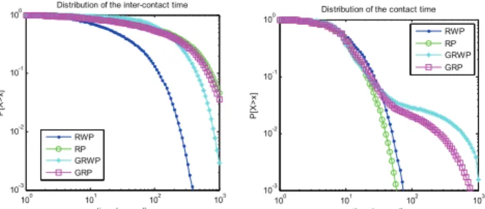
The inter-contact times and contact durations are inherently dependent of the peer movements defined by the considered mobility model. To observe the distribution of inter-contact times and contact durations generated by the four mobility models considered in this study, we ran 50 simulations, each of them with duration of 1000 seconds. Figure 1 and Figure 2 give the contact time distribution and inter-contact time distribution in different coordinate systems. In Fig. 1 left, we can see that the four mobility models’ inter-contact time distribution resembles an exponential distribution. In Fig. 1 right, the contact time distributions show a more marked difference. The two individual mobility models’ curves are still exponential-like curves, but the group models look like a power law. In Fig. 2 we can see the difference between the curves more clearly, using semi-log coordinate system. The exponential nature of the inter-contact time shown in Fig. 1 left is confirmed by the linear shape of the distributions reported in Fig. 2 left.
In terms of the probability of the inter-contact time being larger than a certain time x, the results of the four mobility models are as follows:
(9)
Smaller probability means that in the corresponding mobility model contact events occur frequently, which corresponds to a larger degree of randomness in the nodes mobility patterns. In this sense, we see that the individual mobility model RP proposed in [1] and its corresponding group mobility model GRP proposed here are characterized by a smaller degree of randomness than the other two models, thus taking into account pedestrian or social behavior in a more realistic way.
Figure 1. Inter-contact time cdf and contact time cdf in log-log coordinates.
Figure 2. Inter-contact time cdf and contact time cdf in semi-log coordinates.
IV. SIMULATION RESULTS
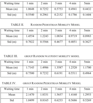
We assume the user can wait at the same position for a period of time long enough to obtain good location estimation, i.e. the final error can meet his requirement. Figure 3 gives a localization error example under RWP mobility model. From it, we can notice that the localization error curve reaches an accuracy threshold as waiting time increases. The horizontal dash line is the mean accuracy. It is computed as the mean of the error curve between times [30sec 120sec] where 30 seconds is the default warm-up time. In Tables 1 to 4, by running 50 times the simulation with different random seeds, we compare the effect of the waiting time on the final localization precision for each different mobility models. As expected, from these tables, we can see that the mean localization error decreases as the waiting time increases. In fact, 2 minutes are enough to achieve satisfying localization. For example, in terms of RWP, within 2 minutes the mean accuracy is about 1 meter.
In Fig. 4, a comparison among different mobility models is shown using the weighted LMI+barycenter localization method (waiting time=120 seconds). In terms of the mean localization error, the curve based on RWP is very often below 1 meter. This indicates that under RWP model our weighted localization scheme works quite well. The curve based on RP also gives us a good result. Most of the values are below 2 meters. In contrast, on the two curves based on group mobility models, such as GRP and GRWP, values are usually less than 3 meters, which can be considered an acceptable performance for most applications.
The weighted LMI+barycenter mean error curve increases in the following order: RWP, RP, GRWP and GRP. The good performance of RWP is due to its randomness and the known issue that with this model mobile nodes are more likely to go through the center of the area, exactly where the user is located. Therefore during the waiting time, the user can almost always find position information of peer nodes available
100 101 102 103 10-3 10-2 10-1 100 time (second) P[ X> x]
Distribution of the inter-contact time
RWP RP GRWP GRP 100 101 102 103 10-3 10-2 10-1 100 time (second) P[ X > x]
Distribution of the contact time RWP RP GRWP GRP 0 200 400 600 800 1000 10-3 10-2 10-1 100 time (second) P[ X> x]
Distribution of the inter-contact time RWP RP GRWP GRP 0 200 400 600 800 1000 10-3 10-2 10-1 100 time (second) P[ X>x ]
Distribution of the contact time RWP RP GRWP GRP
although the passing through peers’ number will be different at different time. Compared with RWP, the RP’s randomness is lower. And they don’t always have the opportunity to pass through the center of the simulation area therefore it may happen that no peers are in the user coverage range. This is why the accuracy obtained from RP is slightly lower than RWP. This problem is magnified in the group models GRWP and GRP. When nodes move in group, the user experiences different situations: sometimes a lot of nodes communicate with it, sometimes no one is in the coverage range. The time interval in which the user can’t find even one peer will be even longer than these two individual mobility models since these nodes begin to move in group. This will decrease the accuracy further.
Figure 3. A localization error curve example of RWP (waiting time=120 sec and warmup time=30 sec).
TABLE I. RANDOM WAYPOIT MOBILITY MODEL
Waiting time 1 min 2 min 3 min 4 min 5min Mean (m) 1.0648 0.7252 0.5753 0.4941 0.4432
Std (m) 0.5540 0.2961 0.2152 0.1786 0.1604
TABLE II. RANDOM PEDESTRIAN MOBILITY MODEL
Waiting time 1 min 2 min 3 min 4 min 5min Mean (m) 1.4554 1.2243 1.0834 0.9719 0.8983
Std (m) 0.7022 0.5566 0.4677 0.4051 0.3627
TABLE III. GROUP RANDOM WAYPOINT MOBILITY MODEL
Waiting time 1 min 2 min 3 min 4 min 5min Mean (m) 1.7143 1.4986 1.3587 1.2520 1.1700
Std (m) 0.7500 0.7232 0.6191 0.5511 0.4964
TABLE IV. GROUP RANDOM PEDESTRIAN MOBILITY MODEL
Waiting time 1 min 2 min 3 min 4 min 5min Mean 2.1470 1.8331 1.5657 1.4160 1.2953
Std 1.0499 0.8165 0.6233 0.5686 0.5269
Figure 4. Weighted LMI+barycenter mean error over 50 experiments (waiting time = 120 seconds).
V. RELATED WORK
In [10] Doherty et al. pioneered the semi-definite programming (SDP) method in localization problem. The localization problem is tried to be considered as a bounding problem containing several convex geometric constrains with the mathematical representation of linear matrix inequalities (LMI). However, in this paper no mobility is applied. Nodes are assumed to be static. The Centroid localization method [11] is developed to estimate the user’s location by computing the barycenter of all the positions received from those fixed beacon nodes. Byplacing four beacon nodes at four corners of a square testing area, an average localization accuracy of with the standard deviation of can be obtained. However, in practice, a uniform placement is not always feasible. To find the optimum deployment of those beacon nodes for a given application may consume a lot of labor. In the APIT method [12], a user chooses three beacon nodes around him as the triangle vertex point and uses the APIT algorithm to test if he is lying in the triangle. If the APIT test can be passed, i.e., at least one node’s signal is becoming stronger when the user move towards any direction, the barycenter of the triangle will be taken as the location estimation of the user. Continuously, another different three nodes will be chosen to face the APIT test again. If the new test can also be passed, the barycenter of the intersection of the triangles will be used. By analogy, the user will repeat this APIT test until all combinations are exhausted or the satisfying accuracy is achieved. It is noticeable that since the APIT test is used under the condition of static beacon nodes, accomplishing it is still not an easy thing. Even there are special cases in which APIT test can’t supply a correct examination about whether the user is resident in the triangle he chooses: experiments in [12] shows that APIT test may fail in less than 14% of the cases. Other research works jointly solve the time synchronization and localization problems. For instance, Enlightness [13] relies on the availability of beacon nodes (at least 5% of the nodes) providing absolute time and space information, like the GPS in outdoor environments. Enlightness combines recursive positioning estimation [14] with a clock offset estimation scheme based on the measure of beacon packet delays and timestamps. 0 20 40 60 80 100 120 0 0.5 1 1.5 2 2.5 3 3.5 4 4.5 5 Time (sec) E rror (m et er)
Weighted LMI+Barycenter estimation error
0 5 10 15 20 25 30 35 40 45 50 0 0.5 1 1.5 2 2.5 3 3.5 4 4.5 5 Experiment # M ean err or ( m et er s) RWP RP GRWP GRP
VI. CONLUSION AND FUTURE WORK
In this paper we have demonstrated the impact of the mobility model used on the evaluation of the accuracy of our weighted LMI+barycenter localization scheme. The obtained accuracy varies from below 1 meter to below 3.5 meters using the same setup with different mobility models. Taking into account groups decreases the performance. However, the obtained accuracy is still acceptable in many scenarios.
It should be noted that in [4] the real traces from Dartmouth College and UCSD show a power law distribution with respect to inter-contact time. From this point of view, it may imply that the two group models in this paper are still not the most realistic ones. The reason may lie in the assumption that nodes are not allowed to move among different groups. This will be improved in our future work. However, they take into account many features that the individual models do not consider, making results more accurate.
In the future developments, we will consolidate this work by relaxing a number of assumptions. We will investigate the relationship between the monitored RSS and a maximum distance for WiFi radios. We will introduce a more realistic communication channel taking into account noise and interferences, and drifting self-estimations of peer positions with periodic reset, and exploit new public mobility traces.
ACKNOWLEDGMENT
This work was partly supported by the European Commission in the framework of the FP7 Network of Excellence in Wireless COMmunications NEWCOM++ (contract n. 216715) and by the French ANR FIL project. The authors would like to thank E. Conchon, A. Bardella and F. Fabbri for valuable discussions on this topic.
REFERENCES
[1] G. Kang, T. Pérennou, M. Diaz, “Barycentric Location Estimation for Indoors Localization in Opportunistic Wireless Networks,” in Proc. of the Second International Conference on Future Generation Communication and Networking (FGCN 2008), Sanya, China, 2008. [2] J Broch, DA Maltz, DB Johnson, YC Hu, J Jetcheva,” Multi-hop
wireless ad hoc network routing protocols”, in Proceedings of the ACM/IEEE International Conference on Mobile Computing and Networking (Mobicom 1998), pages 85-97, 1998.
[3] Y. Ko and N.H. Vaidya, “Location-aided routing (LAR) in mobile ad hoc networks,” in Proceedings of the ACM/IEEE International Conference on Mobile Computing and Networking (Mobicom), pages 66-75, 1998.
[4] A. Chaintreau, P. Hui, J. Crowcroft, C. Diot, R. Gass, and J. Scott, ”Pocket Switched Networks: Real-world mobility and its
consequences for opportunistic forwarding,” Technical Report UCAM-CL-TR-617, University of Cambridge, Computer Laboratory, February 2005.
[5] Francesco Zorzi, GuoDong Kang, Tanguy Pérennou and Andrea Zanella, “Opportunistic Localization Scheme Based on Linear Matrix Inequality”, in Proceeding of IEEE International Symposium on Intelligent Signal Processing (Wisp 2009), Budapest, Hungar
[6] E. de Silva and M. Stumpf, “Complex networks and simple models in Biology”, J. R. Soc. Interface, 2 (2005), pp. 419-430.
[7] N. Przulj, D. G. Corneil, and I. Jurisica, “Modeling interactome:Scale-free or geometric?”, Bioinformatics, 20 (2004), pp. 3508-3515. [8] D. J. Watts and S. H. Strogatz, “Collective dynamics of 'small-world'
networks”, Nature, 393 (1998), pp. 440-442.
[9] M.E.J. Newman and M. Girvan. “Finding and evaluaing community structure in networks”. Physical Review E,68,2003.
[10] L. Doherty, K. S. J. Pister, and L. E. Ghaoui, “Convex position estimation in wireless sensor networks,” in Proc. of the Twentieth Annual Joint Conference of the IEEE Computer and Communications Societies (IEEE INFOCOM 2001), Anchorage, USA, 2001, pp. 1655-1663.
[11] Nirupama Bulusu, John Heidemann and Deborah Estrin, “GPS-less low cost outdoor localization for very small device”, IEEE Personal Communications Magazine, 7(5):28-34,October 2000.
[12] Tian He, Chengdu Huang, Brian M. Blum, John A. Stankovic, Tarek Abdelzaher, “Range-free localization schemes for large scale sensor networks”, in Proc. of the Ninth Annual International Conference on Mobile Computing and Networking (Mobicom 2003), San Diego, USA, September 2003.
[13] Azzedine Boukerche, Horacio A.B.F. Oliveira, Eduardo F. Nakamura, and Antonio A.F. Loureiro. “Enlightness: An enhanced and lightweight algorithm for time-space localization in Wireless Sensor Networks”, in Proc. of IEEE Symposium on Computers and Communications (ISCC 2008), Marrakech, Morocco, July 2008, pp. 1182-1189.
[14] Joe Albowicz, Alvin Chen, and Lixia Zhang, “Recursive position estimation in sensor networks”, in Proc. of the 9th International
Conference on Network Protocols (ICNP 2001), Riverside, USA, November 2001, pp 35-41.
[15] Mirco Musolesi, Cecilia Mascolo, “A community based mobility model for ad hoc network research”, in Proceedings of the 2nd international Workshop on Multi-Hop Ad Hoc Networks: From theory To Reality (REALMAN '06), Florence, Italy, May 2006, pp 31-38.
[16] Mirco Musolesi, Stephen Hailes, Cecilia Mascolo, “An ad hoc mobility model founded on social network theory”, in Proceedings of the 7th ACM international symposium on Modeling, analysis and simulation of wireless and mobile systems, October 04-06, 2004, Venice, Italy.
[17] P. Biswas and Y. Ye, "Semidefinite programming for ad hoc wireless sensor network localization," in Third International Symposium on Information Processing in Sensor Networks (IPSN 2004), 2004. [18] P. Biswas, T.-C. Liang, T.-C. Wang, and Y. Ye, “Semidefinite
programming based algorithms for sensor network localization,” Dept of Management Science and Engineering, Stanford University, submitted to ACM Transactions on Sensor Networks, Tech. Rep., October 2005