CODE-DIVISION MULTIPLEXING
by
Ceilidh Hoffmann
submitted to
the Department of Electrical Engineering & Computer Science
as partial fulfillment of the requirements for the degree of
Doctor of Philosophy
at the
MASSACHUSETTS INSTITUTE OF TECHNOLOGY
September 2004
@Massachusetts Institute of Technology, MMIV
All rights reserved.
The author hereby grants MIT permission to publicly reproduce and distribute paper and electronic forms of this document in whole or in part.
Author's Signature:
Department of Electrical Engineering and Computer Science
Certified by:
Kai-Yeung Siu Thesis Supervisor)
Accepted by: MASSACHUSETTS INSTITTE OF TECHNOLOGYOCT 2
9
2004
LIBRARIES
Arthur C. Smith
Chair, Department Committee on Graduate Students
CODE-DIVISION MULTIPLEXING
by
Ceilidh Hoffmann
Submitted to the Department of Electrical Engineering and Computer Science on August 31, 2004,
in partial fulfillment of the requirements for the degree of Doctor of Philosophy ABSTRACT
We study forward link performance of a multi-user cellular wireless network. In our proposed cellu-lar broadcast model, the receiver population is partitioned into smaller mutually exclusive subsets called cells. In each cell an autonomous transmitter with average transmit power constraint communicates to all receivers in its cell by broadcasting. The broadcast signal is a multiplex of independent information from many remotely located sources. Each receiver extracts its desired information from the composite signal, which consists of a distorted version of the desired signal, interference from neighboring cells and additive white Gaussian noise. Waveform distortion is caused by time and frequency selective linear time-variant channel that exists between every transmitter-receiver pair.
Under such system and design constraints, and a fixed bandwidth for the entire network, we show that the most efficient resource allocation policy for each transmitter based on information theoretic measures such as channel capacity, simultaneously achievable rate regions and sum-rate is superposition coding with successive interference cancellation. The optimal policy dominates over its sub-optimal al-ternatives at the boundaries of the capacity region. By taking into account practical constraints such as finite constellation sets, frequency translation via carrier modulation, pulse shaping and real-time sig-nal processing and decoding of finite-length waveforms and fairness in rate distribution, we argue that sub-optimal orthogonal policies are preferred. For intra-cell multiplexing, all orthogonal schemes based on frequency, time and code division are equivalent. For inter-cell multiplexing, non-orthogonal code-division has a larger capacity than its orthogonal counterpart. Among intra-cell orthogonal schemes, we show that the most efficient broadcast signal is a linear superposition of many binary orthogonal waveforms. The information set is also binary. Each orthogonal waveform is generated by modulat-ing a periodic stream of finite-length chip pulses with a receiver-specific signature code that is derived from a special class of binary antipodal, superimposed recursive orthogonal code sequences. With the imposition of practical pulse shapes for carrier modulation, we show that multi-carrier format using co-sine functions has higher bandwidth efficiency than the single-carrier format, even in an ideal Gaussian channel model. Each pulse is shaped via a prototype baseband filter such that when the demodulated signal is detected through a baseband matched filter, the resulting output samples satisfy the General-ized Nyquist criterion. Specifically, we propose finite-length, time overlapping orthogonal pulse shapes that are g-Nyquist. They are derived from extended and modulated lapped transforms by proving the equivalence between Perfect Reconstruction and Generalized Nyquist criteria. Using binary data mod-ulation format, we measure and analyze the accuracy of various Gaussian approximation methods for spread-spectrum modulated (SSM) signalling. We show that both high rate techniques -parallel chan-nel, single gain and single chanchan-nel, reduced gain- are equivalent under the Gaussian model with or without multipath fading. For seamless multiplexing of SSM channels of various rates, we propose a flexible scheduling policy that removes code blocking and affords statistical multiplexing by dynamically reassigning signature codes. The algorithm is able to support both bursty and constant-bit rate connec-tions without code tree partitioning.
p e b n k p p ag e g e k p e b b l a n k n e) p e b n
k-4
b b Ia n n k b b Ia n n kACKNOWLEDGMENTS
During my stay for the past several years at MIT, I was fortunate to have met and become acquainted with the following wonderful and amazing group of intellectuals. I take this opportunity to thank each and every one of them: My thesis committee members Profs. Dave H. Staelin and Franz Kaertner, and my thesis advisor Dr. Kai-Yeung (Sunny) Siu. Sunny was instrumental in getting me into the research project I was most interested in. My knowledge and interest in networking and higher layer communica-tion protocols were instilled by him. He is my advisor, a good friend and a close confidant. Prof. Staelin has truly been a model professor in giving me advice and encouragement to keep marching ahead. Prof. Kaertner is the sweetest and kindest professor I met at MIT My sincere gratitude goes to my technical examination committee members Profs. G. Dave Forney, Vahid V Tarokh, Jeff H. Lang, Vincent V Chan and Jeffrey H. Shapiro. I am very grateful to Prof. Forney for the time he spent helping me prepare my exam presentation. He clearly showed me the difference between good and great. I also wish to thank my graduate counsellor Prof. Dimitri Bertsekas for his guidance over the years, NTT DoCoMo of Japan for providing the grant that made it possible to conduct research in a wide variety of topics that subsequently lay the seeds for my thesis, and Prof. Gilbert Strang for being a model teacher and whose course in wavelets and filter banks sparked my interest in that subject. My attendance and knowledge gained in his course invariably changed the direction and focus of my thesis. I am indebted to my col-leagues Drs. Mingxi Fan and Anthony Kam for their collaborative work in Chapters 6 and 7. I thoroughly appreciate and respect our diverse backgrounds and the synergy we manage to create in 1-107. Above all, I would not have made it through all the ups and downs without the support and motherly concern of Ms. Marilyn Pierce of EECS, especially at times when I was on the road performing my Hudinic acts.
On a personal note, the following people have profoundly impacted, and ultimately guided me -one way or the other- in my making key decisions that would forever alter my life: All my family members
including Grandma, Hans, and Bob, Drs. Howard Heller, Peter Kassel, Stephan Kurtz and Patient Advo-cate Anne Boppe, and lastly Mr. Ravi Agarwal. I don't need to spell out how much you mean to me.
Finally, my faintest whispering thank you to Duo for all the love, sadness and memories. I once read that it takes more than a good memory to have good memories. I will cherish each and every moment I had with you. You are my everything, my Immortal....
C. H.
cth@alum.mit.edu Boston, MA
6
This document is typeset in Charter font using WinEdt (v.5) text editing software. The final
BTj'EX
file is compiled with MikTEX (v.2.4) text formatting package in PC Windows environment. It is equivalent to the standard TEX2ppackage. All drawings are sketched in AutoCAD LT and then converted to Encapsulated Postscript (.eps) files. All relevant computer files (.tex, .dwg and .eps) used in the generation of printer-friendly files -. pdf and .ps files- are contained in a CD-ROM that is submitted along with this paper copy.To NICK, for making me see that
once in life,
8 b b II 1 b l a n k b l a n k n n k k P p page page g g e e b b I a n k n p k p page page g g b e b b l a n k b l a n k n n k k
CONTENTS
Abstract 3
1 Introduction 23
1.1 Historical Perspective and Motivation . . . 24
1.2 Definitions and Network Models . . . 27
1.3 Problem Statement . . . 30 1.3.1 Optimality Criteria . . . 31 1.4 System Model . . . 37 1.5 Thesis Summary . . . 39 1.6 Organization . . . 40 1.7 A Note on Nomenclature . . . 42
2 Fading Phenomena And Models 49 Summary . . . 49
2.1 Fading Channel Characteristics . . . 50
2.2 Equivalent Baseband Representation . . . 55
2.2.1 Frequency Resolution . . . 56 2.2.2 Time Resolution . . . 58 2.2.3 Wide-Sense Stationarity . . . 60 2.2.4 Uncorrelated Scattering . . . 61 2.2.5 WSSUS Channel . . . 63 2.3 Classification of Fading . . . 63
2.3.1 Short-Term vs. Long-Term Fading . . . 64
2.3.2 Severity of Fading . . . 67
2.3.3 Slow vs. Fast Fading . . . 69
2.3.4 Frequency Flat vs. Selective Fading . . . 71
Notes and References . . . 74
Appendix 2A - Statistical Distributions for Fading Envelope . . . 75 9
CONTENTS
Appendix 2B - Derived Distributions . . . 89
3 Cellular Broadcast Channel
Sum m ary . . . . 3.1 Classification of Multi-User Channels . . . . .
3.1.1 Input-Output Device . . . .
3.1.2 Multi-Terminal Cooperation . . . .
3.1.3 Transition Probability Function . . . .
3.1.4 Broadcast Channel . . . .
3.1.5 Degraded Broadcast Channel . . . . .
3.1.6 Interference Channel . . . . 3.1.7 Composite Channel . . . .
3.1.8 Cellular Broadcast Channel . . . .
3.1.9 Continuous-time Bandlimited Channel 3.2 Single-Cell Channel Capacity . . . .
3.2.1 AWGN Only Channel . . . .
3.3 Channel Multiplexing in Cellular Environment 3.4 Cellular Radio Capacity . . . . 3.4.1 Average Carrier-to-Interference Ratio .
3.4.2 Radio Capacity: FDM/ODM vs. N-CDM/O-CDM . Notes and References . . . . Appendix 3A - Hexagonal Cellular Geometry . . . . Appendix 3B - Achievable Rate Regions: FDM >N-TDM . . .
4 Signature Waveforms and Sequences
Sum m ary . . . . 4.1 Correlation Properties of Continuous-Time Signals . . .
4.1.1 Aperiodic Cross-Correlation . . . . 4.1.2 Periodic Cross-Correlation . . . . 4.1.3 Partial Cross-Correlation . . . . 4.1.4 Periodic, Aperiodic and Partial Auto-Correlation . 4.2 Correlation Properties of Discrete-Time Sequences . . . .
4.3 Signature Waveforms . . . . 4.3.1 Periodic Correlation . . . . 4.3.2 Aperiodic Correlation . . . . 4.3.3 Partial Correlation . . . . 10 95 95 96 97 97 .100 .102 .104 .105 .107 .108 .114 .117 .119 .135 .138 .138 .140 .142 .143 .158 161 .161 .162 .164 .165 .166 .168 .169 .169 .171 .172 .174
.
.
.
.
CONTENTS
4.4 Pseudo-Random Binary Codes . . . 176
4.4.1 Orthogonality . . . 176
4.4.2 Level-Shifting . . . 177
4.4.3 Properties of Signature Binary Sequences . . . 179
4.4.4 PN Sequence Postulates . . . 180
4.4.5 Comments on Pseudo-Randomness . . . 181
4.4.6 Maximal-length Binary Sequences . . . 182
4.5 Binary Orthogonal Codes . . . 185
4.5.1 Sylvester-type Orthogonal Codes . . . 186
4.5.2 Properties of Walsh sequences . . . 187
4.5.3 Orthogonal Binary Code Tree . . . 189
4.6 Superimposed Orthogonal Binary Codes . . . 193
4.6.1 Correlation Properties . . . 194
4.7 Comments on Cross-Correlation of Signature Sequences . . . 197
4.7.1 Correlation Zones . . . 198
4.8 Correlation Properties of Other Important Signals . . . 199
4.8.1 Frequency-Shifted Signals . . . 200
4.8.2 Time-Shifted Signals . . . 201
4.8.3 Time- and Frequency-Shifted Signals . . . 201
Notes and References . . . 203
Appendix 4A - Generation of Binary Orthogonal Codes . . . 204
5 Time-Bandlimited Pulse Design Summ ary . . . . 5.1 Time-Frequency Duality . . . . 5.2 Power Spectral Density . . . . 5.2.1 Deterministic Signals . . . . 5.2.2 Random Processes . . . . 5.3 Nyquist Criterion for Zero Interference 5.3.1 Single-Carrier Nyquist Criterion 5.3.2 Multi-Carrier Nyquist Criterion 5.3.3 Orthogonality Criterion . . . . . 5.4 Perfect Reconstruction Criterion . . . . . 5.4.1 Sampling Theorem Revisited . . 5.4.2 5.4.3 5.4.4 Equivalent Discrete-time Represen Discrete-time Generalized Nyquist Multi-Rate Filter Bank Design . . 211 . . . 2 1 1 . . . 2 12 . . . 2 14 . . . 2 1 5 . . . 2 1 6 . . . 2 1 9 . . . 2 2 0 . . . 2 2 4 . . . 2 2 5 . . . 2 2 9 . . . 2 3 0 tations . . . 232 Criterion . . . 240 . . . 2 4 3 11
12 CONTENTS 5.4.5
5.4.6 5.4.7
Key Observations . . . . Polyphase Decomposition and Fast Comp Bandwidth of Real vs. Complex Carrier M
5.5 Prototype Window Design . . . .
5.5.1 Time-Limited Pulses . . . .
5.5.2 Time-Band-Limited Pulses . . . . Notes and References . . . .
6 Multi-Rate Transmission Schemes
Sum m ary . . . .
6.1 Multi-Rate Transmission Techniques . . . . 6.1.1 System Model . . . .
6.2 BER Analysis of Single-Carrier CDM Channels . 6.2.1 STD-CDM Interference Channels . . . . 6.2.2 Exact BER Computation . . . .
6.3 Various Gaussian Approximations . . . . 6.3.1 Standard Gaussian Approximation (SGA)
6.3.2 Conditional Gaussian Approximation (CG
6.3.3 Improved Gaussian Approximation (IGA) 6.4 BER Analysis in Flat Fading Channel . . . .
6.5 BER Analysis in Frequency Selective Fading Char 6.5.1 Rake Receiver . . . .
6.5.2 Correlated and Uncorrelated Multipath Ir
6.5.3 Gaussian Approximation of Multi-User In
6.6 Comparative Analysis of BER Curves of Target C 6.6.1 AWGN Only Channel . . . . 6.6.2 Flat Fading Channel . . . . 6.6.3 Frequency Selective Fading Channel . . 6.6.4 Comments on BER plots . . . .
6.6.5 Comments on Numerical Methods for CD Notes and References . . . . Appendix 6A - Linear Transformation of Multi-Code S
.tat.o... 247 utation . . . .251 odulated Signals . . . 252 . . . . . . . . .. . . . 254 . . . . 255 . . . 258 . . . . . . . . .. . . . 263 . 265 . . . . .. . . . .- .265 . . . 270 . . . . . . .. . . .. .. 274 . . . 278 . . . 280 . . . 285 . . . 290 . . . 292 A) . . . 296 . . . 297 . . . 299 nel . . . 301 . . . 304 terference . . . 308 terference . . . 312 DM Users . . . 313 . . . 313 . . . 314 . . . 314 . . . 314 M BER Analysis . . . 319 . . . . . . . . . . .320 . ignals . . . 322
7 Resource Allocation Algorithms
Summary . . . .. .. . . . . . -. 7.1 Orthogonal Variable Spreading Factor Codes . . . .
7.1.1 Code Blocking in OVSF-CDM . . . .
333 -333 .335 .337 CONTENTS 12
CONTENTS 13 7.2 Dynamic Assignment of OVSF Codes . . . .
7.2.1 Horizontal Reassignment . . . . 7.2.2 Vertical Reassignment . . . .
7.2.3 Combined Reassignment . . . .
7.3 DCA Algorithm for Constant-Rate Channels . . . . 7.3.1 Optimal Dynamic Code Assignment Algorithm .
7.3.2 Minimum-Cost Branch Search Procedures . . . 7.3.3 Simulation Model and Results . . . . 7.4 DCA Algorithm for Bursty-Rate Channels . . . .
7.5 DCA Algorithm for Mixed-Rate Channels . . . . 7.6 System Requirements for Code Reassignment . . . . . 7.6.1 Control Signalling for Horizontal Reassignments
7.6.2 Control Signalling for Vertical Reassignments . Notes and References . . . . Appendix 7A - Proof of Theorem 7.2 . . . . Appendix 7B - Proof of Theorem 7.3 . . . . Appendix 7C - Code Patterns . . . . Appendix 7D - Cost Comparison Tables . . . . Appendix 7E - Example of Horizontal Reassignments . . . .
. . . 337 . . . 338 . . . 338 . . . 340 . . . 341 . . . 341 . . . 345 . . . 348 . . . 353 . . . 356 . . . 358 . . . 359 . . . 360 . . . 361 . . . 362 . . . 363 . . . 364 . . . 367 . . . 371 Conclusion 7.6.3 Topics Covered . . . . 7.6.4 Topics not Covered . . . . 7.6.5 Topics of Interest . . . .
Symbols & Notations
Bibliography 375 .375 .378 .379 381 CONTENTS 13 395
b n k p p page page g g e e b page page g g e e b k b l a n k n k 14 CONTENTS n b I a n n
FIGURES
A generic communication system with M source-sink pairs . . . .
Multi-user communication channel models . . . . An aerial view of a densely populated geographical area . . . .
An aerial view of a cellular communication network . . . . Achievable rate pair for a two-user Gaussian broadcast channel . . . .
Assignment of frequency blocks in FDM . . . . Additive Gaussian channel models . . . . Excess bandwidth of transmit signal with pulse shaping . . . . System model of a symmetric cellular broadcast network . . . . Block diagram of a cellular communication system . . . .
Direct and indirect sequencing of a discrete-time information sequence Conventional description of spread-spectrum modulation . . . . Preferred description of spread-spectrum modulation . . . .
. . . 27 . . . 29 . . . 30 . . . 31 . . . 33 . . . 34 . . . 35 . . . 36 . . . 37 . . . 38 . . . 44 . . . 45 . . . 47 1.1 1.2 1.3 1.4 1.5 1.6 1.7 1.8 1.9 1.10 1.11 1.12 1.13 2.1 2.2 2.3 2.4 2.5 2.6 2.7 2.8 2.9 2.10 2.11 2.12 2.13 2.14 2.15 15 Penetration of diffracted signals behind obstructed objects . . . 51
Plot of path loss vs. distance . . . 52
Single scattering with multiple unresolvable paths and no LOS . . . 53
Multiple scattering of multiple resolvable paths with no LOS . . . 54
Multiple scattering of a single path with no LOS . . . 55
Single scattering with multiple unresolvable paths including LOS . . . 57
Doppler Spread function . . . 61
Delay Spread function . . . 62
Localized short-term fading . . . 63
Various fading probability density functions . . . 66
Curve fitting of Rayleigh pdf over empirical data . . . 67
The range of amount of fading (AF) for various distributions . . . 68
LCR and AFD for fading rate measure . . . 70
Frequency selective amplitude response . . . 72
16 FIGURES 2.16 Peak-normalized Gamma pdf with various values for oc and 1P
Central chi-square pdf with various values of r and -. . . . ..
Normalized central chi-square pdf for different r and u- . . . .
Non-central chi-square pdf for different r, t and - . . . . Normalized non-central chi-square pdf for different r, and u-One-sided Gaussian and Rayleigh PDFs . . . . Rayleigh probability density function . . . . Rice probability density function with parameter K . . . . Nakagami-m pdf with parameters Tn and . . . .
Nakagami-q pdf with parameters q and l . . . . Log-normal distribution . . . . Conventional and bipolar Bernoulli and Binomial pdfs . . . .
Symmetric bipolar density functions . . . . Symmetric Binomial PDFs of odd and even lengths . . . . 2.17 2.18 2.19 2.20 2.21 2.22 2.23 2.24 2.25 2.26 2.27 2.28 2.29 3.1 3.2 3.3 3.4 3.5 3.6 3.7 3.8 3.9 3.10 3.11 3.12 3.13 3.14 3.15 3.16 3.17 3.18 3.19 3.20 3.21
3.22 Achievable rate region of Gaussian composite channel . . . .1
Channel as an I/O device . . . 97
Broadcast channel model with n receivers . . . 98
Multiple-access channel model with m transmitters . . . 99
Interference channel model with M transmitter-receiver pairs . . . 99
Broadcast channel as single-input, multiple-output device . . . 103
Physically degraded broadcast channel model with two receivers . . . 104
Cascaded physically degraded broadcast channel . . . 105
Sub-channel blocks with cascaded p-degraded broadcast channel . . . 106
Two types of composite channel models . . . 108
Centralized vs. distributed communication networks . . . 109
Cellular network with hexagonal cells . . . 110
Interference from co-channel cell A at distance Dj . . . 111
Composite channel model with link gains . . . 113
Discrete-time channel with embedded modem . . . .114
Continuous-time I/Q data modulator . . . 115
Continuous-time I/Q data demodulator . . . 117
Gaussian broadcast and interference channels . . . 119
Gaussian composite channel . . . 120
Two-user Gaussian broadcast channel rate region . . . 122
Variable rate partitioning in O-CDM . . . 127
Five different shapes for the Gaussian interference channel ARR . . . 131
16 FIGURES . . . 76 . . . 78 . . . 78 . . . 80 . . . 81 . . . 82 . . . 83 . . . 85 . . . 87 . . . 87 . . . 88 . . . 92 . . . 92 . . . 93 . . . .134
FIGURES 17 3.23 3.24 3.25 3.26 3.27 3.28 3.29 3.30 3.31 3.32 3.33 3.34 3.35 3.36 3.37 3.38 3.39 3.40 3.41 3.42 3.43 4.1 4.2 4.3 4.4 4.5 4.6 4.7 4.8 4.9 4.10 4.11 4.12 4.13 4.14 4.15
Approximate distances between target mobile and co-chann Channel assignment in reuse-partitioned cells for Nr = 3 .
Cellular grid composed of equal-size squares . . . . Aperiodic CC for symbol-time limited waveforms . . . .
Periodic CC for symbol-time limited waveforms . . . .
Beginning and ending epochs of aperiodic CC functions . . . .
Correlation of two waveforms with different periods . . . . Correlation with non-zero offset in time epoch . . . . Partial CC function of two signature waveforms . . . . Overlapping of different data bits in the correlation window . Aperiodic CC for chip-synchronous signature waveforms . . .
Aperiodic CC for chip-asynchronous signature waveforms . . .
Two portions of periodic CC for chip-asynchronous waveforms Conversion from finite binary to antipodal signals . . . . Linear feedback shift-register for ML sequence generation . . . Walsh sequences as chip pulses of length 8 . . . . Walsh sequences as chip pulses of lengths 4 and 8 . . . . Complete and incomplete binary code trees . . . . Hybrid channel multiplexing schemes in cellular network . Maximum relative propagation delay in a cellular network Six co-channel interfering sites belong to kth tier group . . Valid polygons for cell grid . . . . Coverage of hexagonal and square cells . . . . A hexagon and its dimension . . . . Flat-top and flat-side hexagonal grids . . . . Linear hexagonal grid . . . . Identification of hex cells in a grid . . . . Four quadrants in a hexagonal coordinate system . . . . . Rotated hexagonal coordinate system . . . . First and second tier cells . . . . Cellular network with hexagonal cells . . . . Reuse distance between two cells . . . . Various cluster patterns . . . . Enlarged hexagon with area B and radius D . . . . Hexagonal cluster patterns for reuse 7 . . . . Reuse partitioning of hexagonal cells . . . .
. . . 164 . . . 166 . . . 167 . . . 167 . . . 167 . . . 168 . . . 172 . . . 173 . . . 174 . . . 174 . . . 178 . . . 182 . . . 189 . . . 190 . . . 191 . . . . 136 . . . 137 . . . 139 . . . 143 . . . 144 . . . 144 . . . 145 . . . 145 . . . 145 . . . 146 . . . 146 . . . 147 . . . 147 . . . 148 . . . 149 . . . 149 . . . 151 . . . 152 el bases . . . 153 . . . 155 . . . 156 17 FIGURES
18 FIGURES 4.16 4.17 4.18 4.19 4.20 5.1 5.2 5.3 5.4 5.5 5.6 5.7 5.8 5.9 5.10 5.11 5.12 5.13 5.14 5.15 5.16 5.17 5.18 5.19 5.20 5.21 5.22 5.23 5.24 5.25 5.26 5.27 5.28 5.29 5.30
5.31 Kaiser windows of length M = 32 and corresponding frequency plots
Complete binary code tree with 16 leaves . . . 191
Complete binary tree with Hadamard codes . . . 192
Description of binary prefix free codes in tree structure . . . 192
Zero correlation zones . . . 199
Rademacher functions and their products . . . 206
Multiple-access channel model with m transmitters . . . 213
Multiple-access channel model with m transmitters . . . 215
Fourier transform of sinc pulse and its aliased copies . . . 221
Amplitude response of Nyquist pulse in four parts . . . 222
Fourier transform of fully raised cosine pulse and its aliased copies . . . 223
Fourier transform of truncated sinc pulse and its aliased copies . . . 223
Frequency response of sinc-type g-Nyquist pulses . . . 227
Bandwidth of single- and multi-carrier modulated raised cosine pulses . . . 229
Discrete-time I/Q data modulator . . . 232
Discrete-time serial-parallel converter . . . 233
Cascade of delay and downsampling for serial-to-parallel conversion . . . 233
S/P conversion with upsampling for input-output rate matching . . . 234
Discrete-time delta modulator . . . 235
A block diagram of a generic discrete-time multi-channel modulator . . . 235
M-channel carrier-modulated communication system: transmitter . . . 236
First four basis functions of type I DCT . . . 239
First four basis functions of type IV DCT . . . 239
M-channel carrier-modulated communication system: receiver . . . 240
Sub-band processing with M-channel filter bank: analysis . . . 244
Odd and even stacking of bandpass filters . . . 245
Sub-band processing with M-channel filter bank: synthesis . . . 246
Standard form of an M-channel filter bank system . . . 247
Reconfigured form of an M-channel filter bank system . . . 248
Reconfigured form of an M carrier-modulated filter bank system . . . 248
Parallel-to-Serial conversion in discrete time . . . 249
Detailed description of multi-carrier communication system . . . 249
Transparency of the cascaded block of expander and delay chains . . . 250
Bandwidth of real vs.complex carrier modulated signals . . . 252
Complex roots of unity as complex carriers . . . 253
Frequency response of various windows for length M = 32 . . . 256
FIGURES
18
FIGURES 19 Prototype windows . . . .
Orthogonality of MLT synthesis functions and their time offset versions Synthesis basis functions of MLT . . . .
Amplitude response of MLT basis functions . . . .
Synthesis basis functions of ELT . . . . Amplitude response of ELT basis functions . . . .
. . . 259 . . . 260 . . . 261 . . . 261 . . . 262 . . . 262 5.32 5.33 5.34 5.35 5.36 5.37 6.1 6.2 6.3 6.4 6.5 6.6 6.7 6.8 6.9 6.10 6.11 6.12 6.13 6.14 6.15 6.16 6.17 6.18 6.19 6.20 6.21 6.22 7.1 7.2 7.3 7.4 7.5 7.6 7.7 7.8 Binary tree structure of OVSF codes . . . . Similarity between two Walsh coded sequences . OVSF code blocking . . . . Complete overpopulation of OVSF sub-tree . . . . Vertical reassignment of OVSF codes . . . . Extreme case of vertical reassignment: TDM . . . complete Under-population of OVSF sub-tree . . . Cost of reassigning a 4R code . . . . . . . 3 3 5 . . . 3 3 5 . . . 3 3 7 . . . 3 3 8 . . . 3 3 9 . . . 3 3 9 . . . 3 4 0 . . . 3 4 2 CDM of four standard-rate channels . . . 272
CDM of a high rate user using two standard-rate channels . . . 273
CDM of a high rate user using a reduced gain channel . . . 273
Channel multiplexing in CDM base transmitter . . . 274
Data and carrier modulation in CDM transmitter . . . 277
Carrier, SS and data demodulation in a CDM receiver . . . 281
Diversity combining of multi-channel signal . . . 301
Resolvable replicas of a SSM signal and their sampling instants . . . 304
Intersymbol interference caused by a multipath signal with delay t5 > T . . . .307
Uncorrelated self-interference when path delay -ri > T . . . 309
Correlated self-interference when path delay Tjj < T . . . 309
Plot 1 of AWGN-BER versus interference population J . . . 315
Plot 2 of AWGN-BER versus interference population J . . . 315
Plot 3 of AWGN-BER versus interference population J . . . 316
Plot 4 of AWGN-BER versus interference population J . . . 316
Plot 1 of FF-BER versus interference population J . . . 317
Plot 2 of FF-BER versus interference population J . . . 317
Plot 1 of FSF-BER versus interference population J . . . 318
Plot 2 of FSF-BER versus interference population J . . . 318
Constellation rotated Walsh modulated output . . . 330
Constellation of reflected Walsh modulated output . . . 332
Modified model of a SSM communication system . . . 332
20 FIGURES 7.9 7.10 7.11 7.12 7.13 7.14 7.15 7.16 7.17 7.18 7.19 7.20 7.21 7.22 7.23 7.24 7.25 7.26 7.27 7.28 7.29 7.30 7.31 7.32 7.33 7.34
Code pattern description for 8R branches . . . . . Extended code pattern description for 8R branches Grid pattern description for 8R branches . . . . . Flow chart of Proposed DCA algorithm . . . . Plot of blocking probability vs. traffic load for Nmaj Plot of number of reassigned codes vs. traffic load. Plot of blocking probability vs. traffic load for Nmna, Plot of number of reassigned codes vs. traffic load: Buffer queues in parallel OVSF-CDM channels Reassignment of leaf codes to another branch Multiplexing of control and data channels within a Delay of encoded data for Walsh code switching . Generation of virtual codes for bursty connections Code patterns for 4R branches . . . . Code patterns for 8R branches in group 1 . . . . . Code patterns for 8R branches in group 2 . . . . . Code patterns for 8R branches in group 3 . . . . . Code patterns for 8R branches in group 4 . . . . . Code patterns for 8R branches in group 5 . . . . . Code patterns for 8R branches in groups 6 and 7 . Code patterns for 8R branches in group 8 . . . . .
CDM code tree with 64 leaves . . . .
New topology of tree with 8R candidate branches New topology of tree with 2R candidate branches Final topology of tree with 2R candidate branches Reassignment of descendant codes of 8R branch .
. . . 345 . . . 346 . . . 347 . . . 349 = 64 . . . 350 for Nm, = 64 . . . 350 = 256 . . . 351 for Nma = 256 . . . 351 . . . 355 . . . 356 time-slot . . . 358 . . . 359 . . . 360 . . . 364 . . . 364 . . . 365 . . . 365 . . . 365 . . . 366 . . . 366 . . . 366 . . . 371 . . . 371 . . . 373 . . . 373 . . . 373 FIGURES 20
TABLES
1.1 System Parameters of GSM and IS-95 Cellular Networks . . . . 2.1 Characterization of Fading PDFs . . . . 2.2 Relation between Power and Envelope Fading PDFs . . . .
3.1 Effective Reuse Number Neff for Hybird Channel Multiplexing Techniques 4.1 Addition and Multiplication in F2 and D2 . . . .
6.1 Possible outputs of a Walsh modulated sequence . . . . Loss in spectral efficiency due to OVSF code blocking
Loss in spectral efficiency due to OVSF code blocking Cost comparison of 4R branches . . . . Cost comparison of 8R branches in groups 1 & 2 . . . Cost comparison of 8R branches in group 3 . . . . .
Cost comparison of 8R branches in group 4 . . . . .
Cost comparison of 8R branches in groups 5, 6 and 7
. . . 353 . . . 353 . . . 367 . . . 367 . . . 368 . . . 370 . . . 370 21 . . . . 24 . . . . 65 . . . . 89 . . . .141 . . . .176 . . . .323 7.1 7.2 7.3 7.4 7.5 7.6 7.7
b b blIa nk b Ian l n n k p p k p a ge p a ge e e b k page
~
page g g e e blan bn ni n _k_ k 22 TABLES1
INTRODUCTION
In wireless communication, the radio frequency (RF) bandwidth is a premium. The only ef-fective means of maximizing bandwidth utilization is by reusing it over and over again at distant locations. Any conceivable wireless communication system -for example, broadcast radio and television channels, walkie-talkie, Citizen Band radio, Personal Mobile Radio, air traffic control, wireless local area networks etc.- adopts this strategy. In the literature, the precise technical jargon is known as frequency re-use; it is measured in terms of a single parameter called the re-use number Nr. Reuse of bandwidth is also the main culprit of interference in a cellular wireless network. Interference due to frequency re-use is synonymous to bacteria: Without it, the entire cellular network is very inefficient in bandwidth utilization; With it, a carefully designed control mechanism is required to maintain the network in equilibrium. Two mutually exclusive techniques that mitigate signal degradation due to interference are propagation loss and coding. The former is mostly a by-product of geometry while the latter is an application of algebra. Since interference originates from distant transmitters, it can be reduced by increas-ing the distance of separation -but at a cost of lower bandwidth efficiency per transmitter. (This remark is explained in detail in Chapter 3.) Determination of an optimal re-use distance is a difficult task for cellular radio system designers. It is a complex problem involving many interdependent factors such as resource allocation policy, information-dependent coding, data modulation format, characteristics of the propagation medium and the design and complexity of mobile transceiver. The final choices of these factors made by European GSMI and American IS-952 system designers are compared in Table 1.1.
'GSM -Global System for Mobile Communications- is a pan-European cellular mobile radio standard that has
been adopted in all regions around the world with a global market share of over 80% as of year 2003. 2
U.S. IS (Interim Standard) 95 is a cellular mobile radio standard pioneered by Qualcomm Inc. that uses
Table 1.1: System Parameters of GSM and IS-95 Cellular Networks
Parameter GSM IS-95
Channel Multiplexing FDM/TDM (downlink) superimposed O-CDM (downlink) Multi-User Accessing FDMA/TDMA (uplink) PN spread N-CDMA (uplink)
with time advance
Duplex mode frequency division frequency division
Re-use number Nr 4 or 7 1
Carrier Modulation s(t) single-carrier single-carrier Data Modulation g(t) MSK (downlink) QPSK (downlink)
MSK (uplink) O-QPSK (uplink)
Pulse-shaping f(t) Gaussian (BT = 0.3) Root raised cosine (r =0.22)
Coding None Pseudo-Noise Coding
(Information-independent) SF = 2 (dl), SF = 42.67 (ul) Convolutional Coding Tc = 1/2, K = 5 (both links) rc = 1/2, K = 9 (downlink)
(Information-dependent) T, = 1/3, K = 9 (uplink)
Modulation spectral efficiency 0.8 1.6
(bits/symbol)
Bandwidth efficiency Neff 4 1.5
(Effective reuse number)
Please refer to page 381 for acronyms.
1.1
Historical Perspective and Motivation
An alternative to propagation loss for interference suppression is information-independent coding -commonly known as spreading. Its sole purpose is to reduce interference from distant transmitters, not background thermal noise. In contrast, information-dependent coding -which is more commonly known as single-user error control or channel coding- is optimized for de-tection of a signal perturbed with samples of an additive white Gaussian noise process -and to a lesser extent, the suppression of interference. Both error control coding and spreading tech-niques achieve their objectives by expanding the signal transmission bandwidth -relative to the uncoded case- by 1 /Tc and kc respectively. (The parameter rc is the code rate of an error-control code and ke is the excess spreading factor of a signature code sequence.) Claude Shan-non formulated the Channel Coding Theorem by proving that in a single-user AWGN channel, reliable communication -with arbitrarily low error probability- is achievable only through coding. This result is also applicable to a multi-user communication system if the code is op-timized for both AWGN and interference. The construction of such codes and their associated decoding methods remain as the Holy Grail in communication system design. In practice system Introduction 24
designers rely on a cascade of two independent operations: single-user error-control coding to combat Gaussian noise followed by channelization coding for interference suppression. Time-, frequency- and code-division multiplexing schemes are examples of channelization coding in time, frequency and code domains, respectively. When the reuse number N, the coding rate rc and the excess spreading factor kc are taken into account, the transmission bandwidth relative to the uncoded case is increased by
Neff = Nrkc
TC
where Neff is defined as the effective reuse number. If Wto0t is the total allocated RF bandwidth for a cellular network, the usable bandwidth per cell (transmitter) is
We = Wtot/Neff (1.2)
The optimal set of numbers that should be assigned to these three variables in eqn. (1.1) for cellular mobile radio is often a contentious matter debated fiercely in the academic world as well as in the industry. Numerous published articles and texts have compared capacities of GSM and IS-95 networks. Other researchers have analyzed the capacities of generic TDMA-and CDMA-based networks. These comparative results may be biased, unfair or incomplete for the following reasons:
0 GSM vs. IS-95: The comparison of GSM versus IS-95 is not always equivalent to TDMA
versus CDMA because key network design parameters such as data modulation format, channel coding rate and constraint length, voice compression algorithm and receiver ar-chitecture skew the overall network performance. The critical role played by the un-derlying channel multiplexing or multi-accessing method (TDMA or CDMA) is no longer apparent. For example, IS-95 affords a much more powerful convolutional code with a longer constraint length than GSM due to its continuous transmission capability. In con-trast, GSM bursts in TDM/TDMA mode do not allow excessive delay for voice packets. For non-voice applications, it is conceivable that a TDMA system can also use a convolutional code of longer constraint length. In terms of data modulation, GSM designers selected minimum-phase shift keying due to its constant envelope property and equivalence to FM/FSK modulation. The former condition allows the use of non-linear RF amplifiers. The latter condition allows the use of an FM demodulator, either in non-coherent, differ-ential or coherent detection mode. In IS-95, both links adopt spectrally more efficient I/Q modulation formats. Since the power efficiency of RF amplifiers is less critical at the base
site, IS-95 designers opted for QPSK in the downlink. For the uplink, its variant offset QPSK -which has a smaller peak-to-average amplitude ratio than QPSK- was chosen. In terms of pulse shapes, GSM adopts a non-Nyquist Gaussian pulse for its smooth spec-tral roll-off. Its goal is to improve bandwidth efficiency with controlled ISI. In IS-95, root raised-cosine Nyquist pulses are used.
" TDMA vs. CDMA: Analytical results obtained from comparative study of generic TDMA
and CDMA systems may not be directly applicable to practical networks since most the-oretical models assume unconstrained signal design, very long codewords and complex decoding algorithms that may not be realizable in practice. For example, in the one-to-many3 broadcast channel, both TDM (as adopted in GSM downlink4) and orthogonal
CDM (as adopted in IS-95 downlink) have the same achievable rate regions. It is true,
however, that the optimal channel multiplexing protocol -with a larger capacity region than TDM- is a non-orthogonal CDM with successive interference cancellation. However, this is not the chosen protocol for IS-95. In the many-to-one multiple access channel, opti-mal CDMA with maximum-likelihood joint detection has a larger rate region than TDMA. On the other hand, naive CDMA (as adopted in IS-95 uplink) has a smaller rate region than TDMA.
" Downlink vs. Uplink: Cellular networks -like most other communication systems- op-erate in duplex mode; i.e., information is exchanged from a stationary base transceiver to mobile terminals and vice versa. The preferred duplexing mode for cellular networks is frequency-division5 where two disjoint RF bands are assigned for base-to-mobile (down-link) and mobile-to-base (up(down-link) transmissions, respectively Thus, any comparative analysis of TDMA versus CDMA is incomplete unless the study is conducted for both downlink and uplink. The GSM standard has the same TDMA architecture, modulation and coding formats in both links. In contrast, the IS-95 standard applies different channel multiplexing, modulation and coding formats in each link.
" Single (fixed) vs. Multiple (variable) Rates: Most comparative studies focus on TDMA
and CDMA network architectures that support a single class of constant-bit-rate channels only This model is well suited for voice and low-rate data applications. It obviously fails to address the feasibility and complexity issues involved in the support of variable data rates in a single channel over the duration of a connection or among different channels. Most often the added complexity in multi-rate communication is at the receiver. For a base site, transmission at a higher information rate is simply a matter of rate-splitting among several parallel low-rate channels. In TDM/TDMA, multi-rate reception involves signal detection over a longer time window. In contrast, the complexity of a CDM receiver may not scale easily for higher information rates.
Our work herein is another attempt -one among many from various researchers and practitoners- that measures and quantifies the contribution of key parameters of a cellular
3
The one-to-many "broadcast" channel is not the same as "downlink." See Chapter 3 for details.
4
downlink = forward link
5
The other option is time-division duplexing where a single RF band is used. The time frame is divided into two sub-frames, with each sub-frame dedicated to base-to-mobile or mobile-to-base transmission.
Introduction 26
1.2 Definitions and Network Models 27
network architecture design. We limit our scope to communication in the downlink only. We do not in any capacity profess that our models and analytical results are unbiased, fair and com-plete. Nevertheless, we have taken a broad approach in which important design parameters -resource allocation policy and its associated channel multiplexing scheme, carrier and data modulation/demodulation techniques, pulse shaping for spectral containment, peak-to-average transmission ratio and resulting latency bound, receiver complexity and scalability- and their intertwined relationships are all taken into account. Before we begin our quest for the Holy Grail, we review some preliminaries:
1.2 Definitions and Network Models
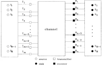
A communication network consists of at least two entities: a source and a sink. Information
is exchanged from a source to a sink. The term "user" is synonymous to "sink." An M-user communication network consists of M source-sink pairs. A source feeds information to its des-ignated transmitter. Communication is established between a transmitter and a receiver through a medium called the channel. The receiver then delivers the message to its associated sink6. The transmitters and receivers play the role of middlemen who help facilitate the transaction -in this case, reliable and efficient communication from a source to its sink.
o I T S1 012 T2 E S2 013 T3 R S3 T4 MR channel Tm~ Rn23 mr-2 M n2 " IM-1 T -1 sM-1 " IM Tm R SM 0 source 0 transmitter * sink E receiver
Figure 1.1: A generic communication system with M source-sink pairs
In general, a communication channel is a two-way street. An example of a two-way chan-nel is the twisted-pair duplex telephone line in which information is sent and received by both entities simultaneously. In the work presented herein, information exchange is simplex -i.e.,
6
1t is assumed that information exchange between a source and its transmitter -and similarly between a receiver and its sink- is instantaneous (zero delay) and error-free.
in one direction only. Therefore every entity is either a source or a sink, but not both.
With stated stipulations, several communication channel models can be envisaged. At a minimum when there are only two entities -a source and a sink- we observe the well-studied single-user channel model. When the source-sink population is much larger, three different types of multi-user channel models -broadcast, multiple-access and interference- can be de-fined. Their distinction is quantified by a single determinant known as cooperation. 'Autonomy" is antonymous to "cooperation." Cooperation is equivalent to pooling of resources; a resource is either a transmitter or a receiver. To facilitate our classification of multi-user channel models, we depict a block form of a generic network with M source-sink pairs in Fig. 1.1. The chan-nel is effectively an input-output (I/O) device with T = m transmitters as inputs and R = n receivers as outputs. Cooperation may exist at the input side among sources or at the output side among sinks. In one extreme all sources and sinks are in full cooperation; this is the de-generate single-user model. In the other extreme with no cooperation at both ends, we obtain the interference channel in which T = R = M. The two remaining channel models are con-structed when there is full cooperation at one (input or output) side only. When there is full output cooperation (R = 1) and autonomous transmitters (T = M), a multiple-access channel is observed. Here, the emphasis is on the receiver since it must -on behalf of all sinks- gather or access information from multiple sources. With full input cooperation (T = 1) and a separate receiver for each sink (R = M), the broadcast channel results. All sources pool a single common transmitter. In return the transmitter broadcasts a compound signal to all users (sinks). All three multi-user channel models are illustrated in Fig. 1.2. A dashed-line block is enclosed among a group of sources or sinks that are cooperating. The compound signal -say, s(t)- is a linear superposition of M time-synchronized, independent signals,
M
s(t) = Y si(t) i=1
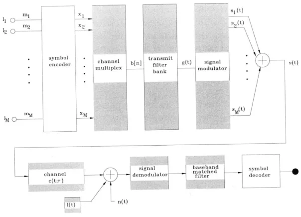
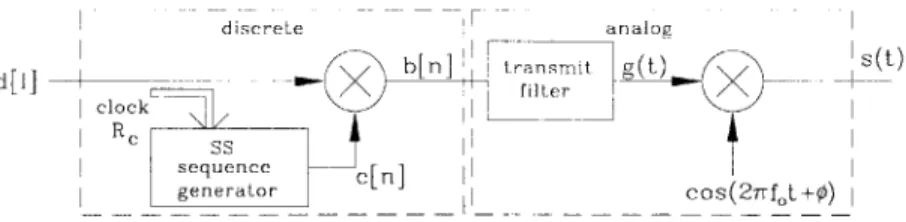
where each elemental signal si(t) is representative of message Mi from source Ii. Channel multiplexing is a transmitter's task of converting independent messages to a broadcast signal:
{mT1,
M2, ... -, MM} -- + s(t), s2(t), ..., )sMt)such that the same broadcast signal is most suitable for transmission to various remotely lo-cated receivers through their respective channels. If an intermediate step where messages are modulated by signature code sequences is included,
{I~n
, M2, ...- ,TM j}
-> bj[j], b2[j],. , bm[j] - s(t) the broadcast signal is said to be code-division multiplexed.Introduction 28
1.2 Definitions and Network Models R S, 0 0 0 0 0 IM-1
I
M MR(a) broadcast model with full input cooperation
Ri U * Si SS?_ S~3 * SM_ * SM
(b) multiple-access model with full output cooperation
29 channel P1 S -.---. Si 0 M-10 SM-1 RM - SM
(c) interference model with no cooperation
Figure 1.2: Multi-user communication channel models
I 1 12 13 channel I, Ti -I TM-1 IM TM channel TI 12 0-TM 0 SM-1 * SM T,
30 Introduction
1.3 Problem Statement
When cooperation is partial, two variations of the interference channel can be deduced. They are labelled collectively as composite channels. We are only interested in the broadcast-interference composite model7 with partial input cooperation (T < M) and autonomous re-ceivers. It mimics the base-to-mobile (downlink) cellular radio propagation channel. Each mobile user or radio receives broadcast signal from its target antenna site as well as interference signals from nearby transmitters. We coin such model the cellular broadcast channel.
S. * 0 00 * Lii. S S S ] 0 * 0 S * - 0 0 * -. . LI * 0 5 * * 0S * 0 0 * 0 __*'~~X' * * 0 0 \\ * 0 Li * * 10 5 @5 0 SI * 0 * 0 / (a) 0 / 0 0 0 * * LII. * 6 * *0 * .3 (b)
Figure 1.3: An aerial view of a densely populated geographical area
Fig.1.3(a) depicts an aerial view of several fixed transmitters (LI) and many scattered sinks
(o) in some densely populated geographical area. If we further assume that an omni-directional antenna is mounted at each transmitter site and neglect physical objects in the propagation medium, the signal strength is the same along the perimeter of a circle of arbitrary radius
-similar to circular (barometric) contours. This "imaginary" coverage area is commonly known as a "cell." As an alternative, it is possible to design a communication network consisting of a single transmitter only with a huge circular footprint (see Fig. 1.3(b)) to accommodate every scattered receiver. This in fact is the paradigm for terrestrial and satellite broadcast services such as radio and television. In both applications, the number of sources (radio or television channels) is much smaller than the number of receivers. This violates our stipulation that a source exists for each sink. If each sink (a listener or a viewer) demands a different TV or radio
7
The other composite channel is multiple-access with interference. A good example of such channel is the cellular uplink. Each base receiver must jointly decode information from its scattered target mobiles in the presence of interfering signals from out-of-cell mobiles.
broadcast channel8, the channel "pipeline" would be very big; i.e., a prohibitively large amount of bandwidth is required. To circumvent the hunger for bandwidth, the region is partitioned into smaller coverage areas. The allocated bandwidth is shared and reused among transmitters. In a nutshell, this is the cellular re-use concept.
Problem Statement:
Consider a large mobile radio communication network depicted in Fig 1.4. Assume the total coverage area is unbounded, and it is partitioned along imaginary lines by concatenation of hexagonal cells of equal size. If the available (radio frequency) band-width is Wtot Hz and the omni-directionally radiated power from each transmitter is limited to P watts, what is the optimal resource allocation policy for each transmitter?
Figure 1.4: An aerial view of a cellular communication network
1.3.1
Optimality Criteria
This begs the question: "How is optimality defined, and what other parameters should be taken into account in selecting the 'best' resource allocation policy for each transmitter?" If optimality is measured in terms of the sum-rate (i.e., the sum of information rates to all users within a cell), then the best strategy is to communicate only with the receiver that maintains
8
The term "channel" is used in different contexts throughout the monograph. Here it refers to a TV or radio station that is tuned in. It also applies to the radio propagation medium through which a signal is transmitted, or a connection -a logical channel such as a frequency band, a time-slot or a code sequence- established between each transmitter-receiver pair.
the best channel response. This policy is evidently unfair to other receivers with poorer respec-tive signal strengths. At the other extreme a "socialist" policy supports the same rate to every receiver regardless of their respective demands. Current cellular systems adopt such a strategy where each circuit-switched channel carries a fixed information rate. This policy is too strin-gent to support various multimedia applications that require variable information rates. Rate adaptation applies not only to the partitioning of the total sum-rate among receivers, but also to dynamic variation of information rate to each receiver throughout the lifespan of a connection.
Achievable Rate Distribution
We may investigate this problem from a different angle. Suppose there is a set of requested rates by receivers:
R* =
(R*,
R*, . . . , R*) We can select an "optimal" resource allocation policyR = (R),R,.. .,R)
that best matches the requested rates with * the minimum mean squared error:
m ine (R* -RP2
" the minimum error in rate-sum:
mine (R - RP)
i=1
" the largest percentage of user population whose requested rates are met:
max i1
where the indicator function 1j = 1 when (Rt > RP) is true, and zero otherwise.
" the largest achievable rate per connection:
maxR, R m ,. , Ro
" the maximization of the minimum rate in all connections:
max{min{R', R,..., Rm
Introduction 32
1.3 Problem Statement 33 R 2 C2 ODM optimal N-CDM N-TDM C R
Achievable rate pair (R1, R2) for a two-user Gaussian broadcast channel. Any rate pair
Figure 1.5: enclosed by the outermost bound (including point A) is achieved by the optimal scheme. Any rate pair, including point B, is achievable by any of the orthogonal schemes.
Depending on the requested rate vector R*, there may be an outright winner or several winners with ties. Consider the capacity-region plot shown in Fig. 1.5. This is the broad-cast capacity of a two-receiver system in an ideal bandlimited channel perturbed by additive white Gaussian noise processes with power spectral densities oaf and o, respectively. The op-timal policy is superposition coding with successive multi-stage decoding. (Details are given in Chapter 3.) The x- and i- intercepts are single-user capacities Cs and Cs of users 1 and 2, respectively. Any rate pair (xi, y ) within the region bounded by the "optimal" curve and the two perpendicular axes can be supported by the transmitter. The figure also gives achievable rate regions (ARR) for several sub-optimal multiplexing schemes. If the target rate pair is point A, then the optimal scheme must be used to meet the demand of all receivers. If the target rate pair is point B, then we have a choice between the optimal and various sub-optimal orthogonal-division multiplexing (ODM) schemes. A similar design option is available for point C where all but naive code-division multiplexing (N-CDM) are good candidates. Moreover, the gap in ARR of the optimal policy over ODM -or likewise the larger rate region of ODM over naive time-division multiplexing (N-TDM)- is proportional to the difference in noise levels af - 2_
In fact when U2 = o2 the optimal and orthogonal-division multiplexing schemes collapse onto
the straight-line rate region of N-TDM. It becomes apparent that measuring the optimality of a resource policy based only a set of simultaneously achievable set of rates is insufficient. We must consider other factors such as:
34
Itouto
Rate Adaptation
During the life of a connection, from the initial handshake to subsequent channel release, the information rate of a user may vary from zero to some upper limit. Referring to Fig. 1.5, at any time instant the supported rate pair may slide from point C to D (or E or F). At another instant it may slide again from D to F. The adaptation of rates between the transmitter and its users must be coordinated dynamically and seamlessly. The break-before-make process -first releasing an existing connection and subsequent acquisition of a new connection- for variable
rate support is not efficient utilization of network resources. If carried out, the total network capacity is reduced due to increased control signal overhead, and above all, the exchange of information is not seamless. With dynamic rate adaptation, a user's information rate is adjusted block-by-block. In time-division multiplexing, a block is a time slot -which is a fraction of time frame allocated to a user. Likewise, in frequency-division multiplexing (FDM) a block is a fraction of the total frequency band. A control flag is appended in each block sent from the transmitter to each user informing the size of the block. Hence we must consider the ease and flexibility of arranging such a procedure in every channel multiplexing scheme.
2 3 2 2 2 3 3 3 fi f2 f3 f4 5 fl f7 f, f, 2 2 2 3 3 3 2 3
Figure 1.6: Assignment of frequency blocks in FDM
Receiver Complexity
For successful coordination of dynamic rate adaptation, a user's receiver must have the capability of accepting -i.e., demodulating, detecting and decoding- a block of variable size. The pertinent issue here is scalability of receiver design for increased information rate. In TDM this is a trivial matter since a larger block implies a longer time window of reception. In a FDM-based cellular network as shown in Fig. 1.6, assigned frequency bands are interleaved such that spectral overlap (i.e., adjacent channel interference) is reduced among frequency bands Introduction 34
allocated to a cell. This strategy precludes the use of a wideband contiguous frequency band
for higher transmission rates. Therefore, an FDM receiver may require a tunable filter with
adjustable (rubber) bandwidth or a set of fixed-bandwidth filters. It is obvious that the latter
option does not scale efficiently.
In the optimal multiplexing policy, the receiver complexity issue is somewhat unique: it is
unrelated to the information rate. Rather it is directly proportional to the number of users and
their relative signal-to-noise ratio (SNR). The user with the lowest noise level has the highest
complexity since it must first decode signals of other users with higher noise levels. The
real-time implementation of such a procedure may not be feasible in a fading environment. We
elaborate on these remarks in Chapter 3. As presented therein, the receiver complexity issue
takes a different flavor when combined with the frequency re-use concept of cellular networks.
Dynamic Resource Allocation
In rate adaptation the aim is to provide rate guarantees on a per-user basis. It is mainly
concerned with the physical layer (e.g., receiver hardware complexity) and the medium-access
layer (e.g., control channel flag) issues. It is a local optimization policy; its interest lies in the
support of rate
Rmax/n
for an arbitrary n > 1. It does not address -or is even concerned
with- the issue of maximizing the overall network information capacity, which is of course
a network layer global optimization problem. This subject of dynamic resource allocation is
broken down into network operations such as call admission control, data channel scheduling
and queuing and prioritization of data packets. The goal is to support a certain pre-defined
level of quality-of-service (QoS) -loosely measured in terms of maximum information rate, the
ratio of maximum to average information rate, call admission and dropping rates- to every
user while maximizing the time-averaged capacity of the entire network. It is well known that
TDM with its bursty transmission property generally has a high ratio of maximum-to-average
information rates. The opposite is true for FDM. In orthogonal code-division multiplexing
(0-CDM), as demonstrated in Chapter 7, the total network capacity also depends on the type of
signature code sequences.
C(f) N(f) N 3 N2 N N4 I N5 frequency frequency (a) (b)
Additive Gaussian channel models Figure 1.7:
(a) frequency selective channel (b) non-uniform Gaussian PSD