HAL Id: hal-01505024
https://hal.archives-ouvertes.fr/hal-01505024
Submitted on 10 Apr 2017
HAL is a multi-disciplinary open access archive for the deposit and dissemination of sci-entific research documents, whether they are pub-lished or not. The documents may come from teaching and research institutions in France or abroad, or from public or private research centers.
L’archive ouverte pluridisciplinaire HAL, est destinée au dépôt et à la diffusion de documents scientifiques de niveau recherche, publiés ou non, émanant des établissements d’enseignement et de recherche français ou étrangers, des laboratoires publics ou privés.
Copyright
United States
Severine Furst, Michel Peyret, Jean Chery, Bijan Mohammadi
To cite this version:
Severine Furst, Michel Peyret, Jean Chery, Bijan Mohammadi. Lithosphere rigidity by adjoint-based inversion of interseismic GPS data, application to the Western United States. Tectonophysics, Elsevier, 2018, 746, pp.364-383. �10.1016/j.tecto.2017.03.015�. �hal-01505024�
LITHOSPHERE RIGIDITY BY ADJOINT-BASED INVERSION OF INTERSEISMIC 1
GPS DATA, APPLICATION TO THE WESTERN UNITED STATES 2
3
Severine Fursta,*, Michel Peyreta, Jean Chérya, Bijan Mohammadib
4
aGéosciences Montpellier, Université de Montpellier, CNRS UMR-5243, 34095 Montpellier, France
5
bIMAG, Université de Montpellier, CNRS UMR-5149, 34095 Montpellier, France
6
*Corresponding author. Email address: [email protected] S. Furst
7 8
ABSTRACT 9
While vertical motion induced by long-term geological loads is often used to estimate the 10
flexural rigidity of the lithosphere, we intend to evaluate the shear rigidity of the lithosphere 11
using horizontal motion. Our approach considers that the rigidity of the lithosphere may be 12
defined as its resistance to horizontal tectonic lateral forces. In this case, a spatial distribution 13
of an effective shear rigidity can be estimated from the analysis of the interseismic velocity 14
fields. We consider the Western United States zone where weakly strained areas (e.g., the 15
Sierra Nevada) are connected with areas of large strain rate (e.g. San Andreas Fault system). 16
By inverting interseismic strain distribution measured by geodetic methods, we infer the 17
effective shear rigidity of the lithosphere. The forward problem is defined using the equations 18
of linear elasticity. The inversion relies on the minimization of the sum of a quadratic measure 19
of the differences between measured and modelled velocity fields. The functional also 20
includes regularization terms for the parameters of the model. The gradient of the functional 21
with respect to the minimization parameters is computed using an adjoint formulation. This 22
permits the treatment of large dimensional minimization problems. Finally, a measure of the 23
uncertainty of our inversion is illustrated through the covariance matrix of the parameters at 24
the optimum. The optimization chart is validated on two synthetic velocity distributions. 25
Then, the effective shear rigidity variations of the Western United States are estimated using 26
the CMM3 interseismic velocities. The inversion displays low effective rigidities along the 27
San Andreas Fault system, the Mojave Desert and in the Eastern California Shear Zone, while 28
rigid areas are found in the Sierra Nevada and in the South Basin and Range. Finally, we 29
discuss the differences between our strain rate and rigidity maps with previously published 30
results for the Western United States. 31
32
Keywords: GPS; interseimic velocity; effective rigidity; global optimization; San Andreas 33
Fault system; uncertainties. 34
35
1. INTRODUCTION 36
Geological strain occurring over millions of years results from the continuous accumulation 37
of anelastic processes in the crust and in the lithosphere in response to plate motion. Active 38
deformation areas are identified by seismicity and geodetic deformation. In active 39
deformation area, the comparison of plates motion from geology and geodesy, at these two 40
different time scales, provides a fair agreement in term of horizontal velocities (Sella et al., 41
2002). Geologic and geodetic comparisons can also be made across active faults using 42
standard models for interseismic strain (McCaffrey, 2005; Meade and Hager, 2005; Savage 43
and Burford, 1973). It appears that most of the documented faults display a close agreement 44
between geodetic and geologic strain rates (Vernant, 2015). 45
From a mechanical viewpoint, the close agreement between short and long-term strain rates 46
(i.e. time scales from 10 yrs to 1 Myrs) probably reflects the stability of the stress balance in 47
the lithosphere under the action of slowly evolving remote forces associated to subduction, 48
basal drag and, more generally, the plate system gravitational potential energy. Under the 49
action of these forces, strain distribution is mostly controlled by the lithospheric strength. By 50
strength we mean the maximum force sustainable by the lithosphere. Like lithospheric stress, 51
lithospheric strength cannot be determined precisely with depth, unless with crude rheological 52
yield strength envelope models (Tesauro et al., 2011). Indeed, a precise strength estimate with 53
depth would require a detailed knowledge of the temperature profile with depth, lithology and 54
water contents, as well as friction law in the brittle domain and temperature dependent viscous 55
laws in the ductile crust and mantle. Therefore, the lithospheric strength can only be 56
approached through its integral measure along depth, with numerical models of the 57
lithosphere. These solve stress equilibrium using elasto-visco-plastic laws with prescribed 58
boundary conditions (Bird and Kong, 1994; Chéry et al., 2001). However, a simplified 59
version of lithospheric strength is embedded in the concept of effective elastic thickness 60
(EET) applied to plate flexure. Indeed, it has been shown that plates submitted to topographic 61
and other internal loads display vertical motions controlled by plate rigidity (Watts, 2001). 62
Combined analysis of topographic and gravimetric signals allows for computing effective 63
elastic thickness and its variation at continental scale (Lowry and Smith, 1994; Pérez-64
Gussinyé et al., 2009). A fair agreement is generally found between heat flow and EET where 65
small values of EET correspond to high heat flow zones. 66
Both lithospheric strength and effective elastic thickness are commonly associated with the 67
long-term behaviour of the lithosphere. However, these concepts can be adapted in order to 68
interpret interseismic geodetic measurements (Chéry, 2008). For a typical time of 10 years of 69
geodetic observation and in the absence of large earthquakes, a linear evolution of GPS 70
motion is often observed. Therefore, a collection of GPS velocities may be used in order to 71
compute strain rate maps at plate scale (Kreemer et al., 2014). Even if this latter analysis is 72
purely kinematic, the resulting geodetic strain rate must satisfy stress equilibrium over the 73
time of observation. In such a problem, the unknown is the incremental lithospheric strength. 74
One example is the spatial variation of the stress change integrated over the depth over the 75
time of GPS observation. The problem can be simplified assuming that lateral strength 76
variation is modulated by geodetic plate thickness (Chéry, 2008). The integrated value of the 77
shear-stress at depth is what we call the effective shear rigidity. It is conceptually similar to 78
the flexural rigidity: the effective shear rigidity expresses the resistance of the lithosphere to 79
lateral forces (unit is N), while the effective flexural rigidity is related to the resistance of the 80
lithosphere to vertical bending (unit is N.m). 81
In Chéry et al. (2011), we proposed a global optimization approach to estimate effective plate 82
rigidity maps by the inversion of a GPS velocity field. The inversion provides a rigidity field 83
realizing a RMS between the observed and modelled velocity fields close to 2 mm/yr for a 84
dataset in southern California. However, we faced difficulties to properly fit high velocity 85
gradients in the vicinity of the San Andreas Fault system. This is because the method did not 86
allow the consideration of large inversion problem and therefore the local spatial density of 87
our model parameters was too low. Moreover, a priori velocity boundary conditions were 88
necessary and no uncertainties estimated. 89
In this paper, we present an enhanced version of the method to address the previous issues: 90
the number of optimization variables can now be arbitrary thanks to the use of an 91
adjoint formulation of the forward problem. This permits high spatial resolution for 92
the rigidity. 93
boundary conditions are not anymore prescribed but now treated as optimization 94
variables as well. 95
uncertainties are calculated for optimal rigidity value. 96
The paper is organized as follows: (1) we describe the new features of the method and we 97
state the differences with respect to Chéry et al. (2011), (2) we demonstrate the efficiency of 98
our new approach on a synthetic dataset that mimics a strike slip fault locked at depth, (3) we 99
propose a refined rigidity map of southern California and we study the sensitivity of the 100
solution of the inversion problem with respect to the location of domain boundaries. Finally, 101
(4) we compare and discuss our results with those already published, both in terms of strain 102
rate maps and effective elastic thickness. 103
104
2. GOVERNING EQUATIONS AND FORWARD MODELLING 105
Geophysical laws provide the mathematical framework to compute the outcome of some 106
physical processes: this is called the forward problem. In other words, the model and its inputs 107
are known and specific data (e.g. seismic, geodetic, or magnetic) are sought thanks to the 108
equations linking the physical parameters to the solution at the observation location. Most of 109
the time, we only have access to the consequences of a physical process (e.g. the geodetic 110
measurements). These consequences need to be inverted to determine the physical properties 111
of the Earth interior (Tomography: e.g. Montelli et al., 2004; Tanaka et al., 2009. Volcanoes 112
and geothermal zones: e.g.; Anderson and Segall, 2013; Dzurisin, 2003; Mossop and Segall, 113
1999. Application to reservoirs: e.g. Hesse and Stadler, 2014). In some cases, there are 114
analytical s
115
the observations. For most geophysical problems, the limited amount of data used to 116
reconstruct a model with infinite degrees of freedom leads to the non-uniqueness of the 117
solution. Consequently, the inverse problem only provides one of the many models that 118
explain the data and has uncertainty because the real data are subject to uncertainties and 119
errors. 120
The effective elastic thickness of the lithosphere can vary laterally due to both elastic 121
properties and the rheological failure properties that limit elastic strength. Flow strength 122
depends on other factors than the temperature. Also, part of the variation imaged by the 123
geodetic technique is probably due to the limits of frictional strength on faults (Bird and 124
Kong, 1994). The thermal plate regime probably exerts a large influence due to the sensitivity 125
of the effective plate rigidity with respect to its temperature profile (Watts, 2001). Here, we 126
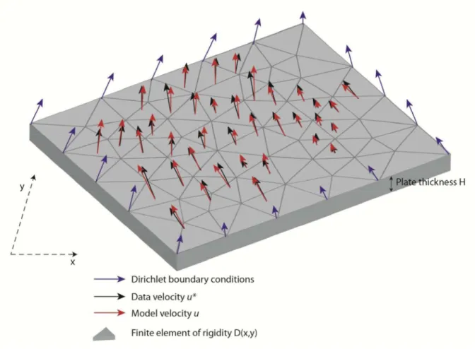
model these rigidity variations as lateral variations of the elastic properties of a plate with 127
constant thickness. Thus, our forward model is made of a domain ( ) symbolizing a 2-D 128
plate, which can deform according to linear and isotropic elasticity (Fig. 1). Along the 129
boundary of the domain , we apply Dirichlet conditions (i.e., in-plane velocities ) and 130
assume free normal traction at the surface of the plate (plane stress assumption). This 131
hypothesis means that strain perpendicular to the plane can occur. The forward model is 132
therefore composed of three equations, the stress equilibrium (Eq. 1), a constitutive equation 133
linking the strain rate to the stress rate for a 2-D plate (Eq. 2) and boundary conditions (Eq. 134 3): 135 on (1) on (2) on (3) where and are the strain- and stress-rate tensors, is the Kronecker delta function, and 136
137
is assumed to be constant and equal to 0.25. The Young modulus remains the only free 138
mechanical parameter in this equation. Since the model is driven by a velocity condition, only 139
. This means that 140
any distribution of the form provides the same velocity field 141
regardless the value of the constant C. For this reason, we define the non-dimensional 142
effective rigidity distribution as where is the minimum value of 143
over the domain. So, all distributions of presented in this paper range from 1 to some 144
maximum values. 145
For a given spatial domain, we generate a uniform 2-D Delaunay mesh composed by 146
triangles. In order to estimate the velocity field at geodetic measurement locations we use 147
the academic 2-dimensional finite element code CAMEF. The code does not incorporate the 148
value of the plate thickness. Therefore, we cannot discriminate plate thickness and elastic 149
properties of the lithosphere from the rigidity values. Hence, fixing an absolute value to the 150
rigidity remains an open problem. Finally, the velocity field produced by the forward model 151
depends on two input parameter sets: the velocity boundary conditions and the 152
distribution of (Fig. 1). Eventually, we try to fit with the observations . 153
154
3. INVERSION METHOD 155
Running the direct problem requires the prescription of the velocity on the boundary nodes 156
and the rigidity for each mesh element. Contrary to the approach proposed in Chéry et al. 157
(2011), the boundary conditions are not imposed anymore in the inverse problem and are 158
treated as optimization parameters. We associate one rigidity parameter to each mesh element 159
leading to a very large optimization problem. Our global optimization algorithm requires the 160
gradient of the functional. We consider an adjoint formulation of the forward model to access 161
this gradient with respect to all the model parameters simultaneously. 162
3.1 Cost function 163
We want to invert observed data and determine the model parameters 164
minimizing the distance (here -norm) between the observed data and the predicted field 165
inside the domain : 166
(4) where is the cost function to minimize, and subscript means that the -norm is 167
weighted by the inverse of the covariance matrix of the geodetic measurements. 168
Geophysical inverse problems are usually ill-posed and need to include a subjective degree of 169
regularisation to achieve relevant geophysical solutions (e.g. Zaroli et al., 2013). We therefore 170
introduce to the cost function two Tikhonov regularization terms to control local fluctuations 171
of the parameter vector (Tarantola, 2004; Tikhonov, 1943). We separate the regularization of 172
the parameters along the boundaries and those associated to the rigidity inside the 173
domain: 174
(5) where and are regularization operators. The former acts over the domain and 175
controls the regularity of the rigidity distribution, while the latter monitors the regularity of 176
the boundary conditions. Both are particular forms of non-linear Laplace-Beltrami operators 177
with a local control of the level of regularization (Mohammadi and Pironneau, 2009). The 178
weights have to be chosen by the user. Series of different optimizations have been run to 179
highlight the effect of on the inversion. By doing so, our goal is to adjust to the data 180
, while preserving some degree of regularity on both the rigidity inside the domain and the 181
velocities along the boundaries. However, for each simulation, we only have the values of the 182
velocities (and not rigidity) to compare with. Hence, adjusting the regularity of the rigidity is 183
largely subjective and we found that using no regularization ( ) for rigidity leads to 184
acceptable spatial rigidity gradients. Hence, in this study, we only consider the regularization 185
term of the boundary conditions. 186
In order to choose , we explore the trade-off between the residual data misfit 187
and the regularization term . This is featured in a trade-off or Pareto 188
curve, which gathers all feasible solutions that cannot be improved in any of the objectives 189
without degrading the other objectives (e.g. Vassilvitskii and Yannakakis, 2005). The 190
selection of an optimally regularized solution depends upon the requirements of a particular 191
study. We will illustrate the impact of the regularization over the boundary conditions for the 192
rigidity inversion in Southern California. 193
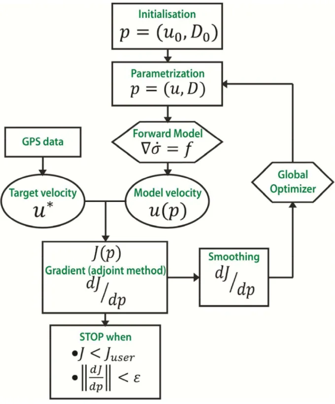
3.2 Global optimization 194
We apply a global optimization algorithm (Ivorra et al., 2013) to iteratively invert interseismic 195
geodetic data. Global optimization is necessary as we have no information on the convexity of 196
the cost function and several local minima can be present. The global optimization strategy is 197
meant to improve the initial condition for classical gradient-based methods looking for an 198
initialization in the attraction basin of the global optimum (Mohammadi and Pironneau 2009). 199
In addition to the Tikhonov regularization mentioned above, the gradient of the functional is 200
smoothed (Mohammadi and Pironneau, 2004, 2009) in order to control the regularity of the 201
parameters. The optimization algorithm ends when the functional or the variations of the 202
gradient are smaller than some user-defined thresholds. A synthetic flow chart of the inverse 203
problem is given in Fig. 2. 204
Functional derivatives computation is done using an adjoint formulation of the forward model 205
(e.g. Plessix, 2006). In most of the inverse problems in geophysics, the cost function cannot 206
be analytically linearized. If a finite difference approach is adopted, the number of forward 207
computations for assessing the gradient of the functional is proportional to the number of 208
parameters. Let us briefly recall the adjoint technique. The gradient of the functional with 209
respect to the model parameters can be expressed as follows: 210
(6) where is the functional, the parameters and the velocity calculated at each node of the 211
mesh. From the equilibrium equation , we incorporate the rigidity matrix and the 212
stress vector in (Eq. 6): 213
Defining the adjoint variable as the solution of the system (because is 214
self-adjoint in our case), we obtain: 215
(8) Consequently, the amount of computation needed to obtain the gradient of the functional 216
mostly corresponds to the solution of one forward model, by opposition to a finite difference 217
scheme which needs a number of forward model solutions equal to the number of parameters. 218
3.3 Model Parameters initialization 219
Real GPS datasets present large spatial variations of density measurements. GPS stations are 220
usually set to observe the velocity gradient around fault zones. Therefore, we usually expect 221
null strain in geographical areas where measurements are sparse. This information can be 222
used to define the initial guess for the lithosphere rigidity in the optimization procedure. This 223
is similar to what is done in topological optimization (e.g. Allaire et al., 2004) where the 224
initial structural rigidity is set to the maximum admissible value. Optimization then aims at 225
making the structure softer and softer. A common problem in mechanical structure design is 226
to optimize the topology of an elastic structure given certain boundary conditions. Optimality 227
implies to minimize the weight, but at the same time, the structure needs to be as strong and 228
rigid as possible. The rigidity of each element is hence reduced at each iteration of 229
optimization when requested. 230
Synthetic and real cases presented in this paper involve rigidity reaching very large values in 231
areas that exhibit little internal deformation. Thus, the rigidity amplitude ranges from a given 232
minimum to infinity in no-deformation zones. This semi-open variation domain is not suitable 233
for numerical search. Consequently, we choose a parametrization design using the 234
compliance, , of the material instead of the rigidity. The compliance is defined over the 235
interval , the lower bound corresponding to a quasi-rigid body. We have considered 236
different values of . It appears that a value of which corresponds to two order of 237
magnitude admissible variation for the rigidity is sufficient to fully capture the range of most 238
strain- Appendix B). This use of
239
compliance insures greater stability of the inversion process. For ease of understanding and 240
interpretation, we express our results in terms of rigidity after the inversion is completed. 241
3.4 Model parameters uncertainty 242
GPS observations are plagued with uncertainty due to various factors: instrumental noise, 243
field measurement procedure, the skill of the operator and local environmental motions. These 244
uncertainties affect in a complex way the GPS time series and generate a coloured noise on 245
positions (Mao et al., 1999). But, these also induce uncertainties on the model parameters 246
determined through our optimization process. For that reason, it is essential to quantify the 247
impact of data uncertainty propagating through the inversion. Hence, the resulting rigidity 248
distribution is complemented with a sensitivity map. 249
To determine the model parameters uncertainties, we link the covariance matrices of the 250
parameters and data. Let us consider the observation (geodetic velocities) as a sum of a 251
- with zero variance (i.e. and an uncertain quantity 252
: . For this sum, the covariance matrix is given by: 253
(9) Because is deterministic, and are independent (i.e. . Therefore, the 254
covariance matrix reduces to: 255
(10) We consider a linear relationship between and :
256
(11) which leads to:
(12) where is the Jacobian matrix made of the derivatives of the velocities at geodetic 258
measurement locations with respect to the model parameters. Similarly to (Eq. 9), we define 259
the covariance matrix of the predicted parameters as: 260
(13) where (the actual values of the parameters) is assumed deterministic. Again, and are 261
assumed independent, and therefore: 262
(14) Finally, equation (Eq. 12) becomes:
263
(15) (16) So, this equation formulates the uncertainty propagation from geodetic measurements to the 264
model parameters via the Jacobian matrix . The construction of this matrix can be performed 265
in two different ways. The simplest approach consists in expressing it analytically as a 266
function of the gradients that have been evaluated during the resolution of the adjoint 267
problem. Indeed, can be explicitly deduced from the equation . This 268
approach is straightforward and theoretically correct, but it is numerically unstable since it 269
involves the inversion of singular matrices. Consequently, it is more robust to build from 270
finite difference computations. This consists in perturbating one parameter around its 271
optimum (typically by 10%), and then computing the perturbation of the predicted velocity at 272
all geodetic measurement locations. This approach is numerically robust because it involves 273
no matrix inversion. With the second member of Eq. 16 in hand, we can now provide an 274
estimation of the variance (diagonal of the covariance matrix) of the optimization variables. 275
In this study the parameter is the compliance with its standard deviation 276
. We define dissymmetric upper and lower bounds around the optimum for 277
the rigidity parameter . To represent the uncertainty on the 278
rigidity ( ) we use the fact that is the inverse of the compliance and therefore: 279
(17) 4. Determination of effective rigidity for a synthetic case
280
Before running our optimization scheme on real cases, we evaluate its efficiency to recover a 281
given rigidity distribution (target rigidity) associated with a specific 2-D velocity field . 282
Surface strain across a locked fault zone can be interpreted either using the concept of a 283
slipping fault zone beneath a locking depth (Savage and Burford, 1973) or by assuming a 284
shear-rigidity variation perpendicular to the fault (Chéry, 2008). Differences and similarities 285
between these models are discussed in this latter paper. According to the variable rigidity 286
hypothesis, we define a target given by: 287
(18) Where is a non-dimensional rigidity, is the distance to the fault and is a characteristic 288
dimension. Solving force balance within such a plate leads to the following fault-parallel 289
velocity field: 290
(19) Therefore, such a velocity distribution is the solution of the spatially variable function of Eq. 291
18 but can also be associated to a screw dislocation at depth (e.g., Savage and Burford, 1973). 292
In the case of active fault systems, is generally associated to a physical locking depth which 293
can be estimated using geodesy and seismology. In the case of the San Andreas Fault system, 294
values of d range from 6 to 22 km depending on the location along the fault and the method of 295
determination (e.g. Smith-Konter et al., 2011). 296
We conduct two tests to verify the ability of the method to retrieve the rigidity distribution 297
given by Eq. 18 for different GPS data sets. We also test different values of (from 2 km to 298
17 km) in order to generate velocity fields commonly observed on the San Andreas Fault. The 299
specific case of fully-creeping faults ( ~0 km) is discussed in Appendix A, with application 300
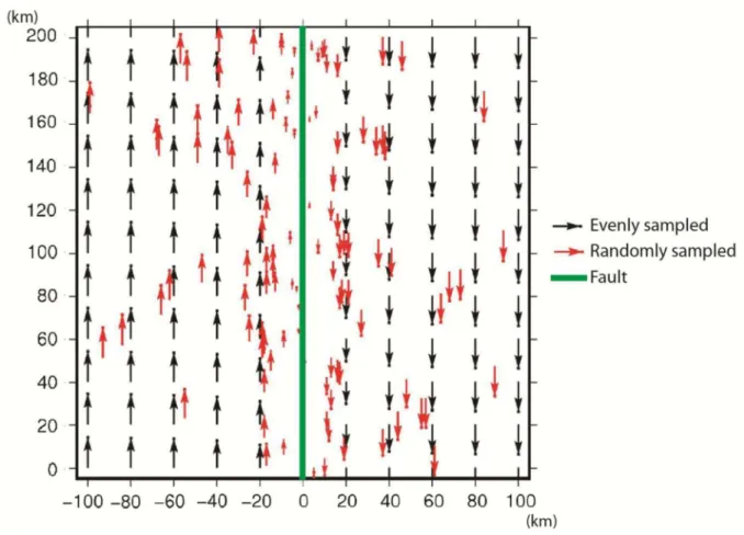
to the SAF segment located North of Parkfield. We focus here on the consequences of 301
processing two different spatial distributions of GPS data: (1) evenly spatially distributed and 302
(2) concentrated near highly strained zones. This corresponds to on site situations (Fig. 3). 303
Both distributions are made of about 120 GPS velocities vectors. 304
Several experiments have been conducted to define an optimal mesh size. On the one hand, 305
the computational time is related to the mesh size. The finer is the grid, the longer will be the 306
optimization (about 60 times longer for a mesh 3.6 times finer). On the other hand, the grid 307
needs to be fine enough to capture the variations of the velocity field, notably close to high 308
velocity gradient areas such as the creep zones of the Parkfield segment. Eventually, a 309
spatially adaptive mesh should be implemented. We choose to work with a mean constant 310
spacing of 20 km. This configuration is generally a good compromise between the number of 311
available geodetic measurements, the number of parameters that need to be adjusted and the 312
size of the object we want to study. 313
For the first case, GPS measurements (black arrows on Fig. 3) are uniformly distributed over 314
the domain, with a constant spacing of 20 km. For the second distribution, we mimic 315
GPS network by producing a velocity field whose spatial density decreases with the distance 316
to the fault. In both cases, the domain is a 200-km square with a 20-km mesh size (394 317
elements). The dextral strike-slip fault (green line on Fig. 3) has a slip rate of 30 mm/yr and 318
is locked at 10 km depth. The admissible values for the non-dimensional relative rigidity 319
range from 1 to 100 (see Appendices A and B for a discussion of such a choice). 320
We apply our optimization algorithm to invert the two velocity fields (Fig. 4 and 5). In the 321
case of the uniform dataset (Fig. 4 a-f), we first compare the synthetic velocities (red dots on 322
Fig. 4e) to the modelled ones (grey dots on Fig. 4e) along a profile (white dashed line on Fig. 323
4a) perpendicular to the fault (black dashed line on Fig. 4a-c). The dataset from the inversion 324
almost perfectly matches the characteristic shape of a 2-D arctangent velocity field given by 325
Eq. 19 (Fig. 4e). The misfit between predicted and theoretical (Fig. 4d) permits to 326
estimate the tendency in over or under estimating in our inversions. Besides, the difference 327
between synthetic and modelled velocities, hereafter called residual velocities, is lower than 328
0.25 mm/yr over the whole domain (Fig. 4c). 329
Contrary to real cases where the true effective rigidity distribution is unknown, synthetic 330
cases allow for testing the efficiency of our inversion method to retrieve the quadratic rigidity 331
field given by Eq. 18. Fig 4a shows the rigidity distribution over the whole domain of 332
analysis, while Fig. 4b shows the uncertainty distribution map and Fig. 4f focuses along one 333
transect across the fault. We can notice that, as expected, the code predicts a low rigidity zone 334
(90% of the elements ranging between 1 and 3) along a 40 km-wide area centred on the fault. 335
Also, increases rapidly with the distance to the fault to reach high values (>30) 60 km from 336
the fault. Associated with these rigidity values, we find uncertainties that are very small where 337
rigidity is small but quite high when the opposite occurs (Fig. 4b). This mainly comes from 338
the predominance of the (squared) rigidity term in Eq. 17. This expresses the fact that, in areas 339
that do not deform significantly, very large values of rigidity are admissible (up to infinity) 340
without modifying significantly the local velocity field. Since our search interval for rigidity 341
is bounded, our optimal solutions tend to underestimate the real rigidity in non-deforming 342
areas. This can be seen far from the fault in all the synthetic cases presented in this study (Fig. 343
4, 5, A.1 and A.2). Finally, we find that, within the uncertainties estimated by our method 344
(paragraph 3.4), our predicted rigidity distribution fits its theoretical value. This is clearly true 345
along the transect crossing the fault on Fig. 4f. 346
For a data set whose density decreases with distance to the fault (Fig. 5a-f), we observe the 347
same ability for the optimization algorithm to retrieve an arctangent-shaped velocity field 348
(Fig. 5f) and this despite sparse data away from the fault. In this synthetic case, some 349
elements of the grid contain more than one velocity, making the capture of very local velocity 350
gradients difficult if not impossible using one single rigidity parameter over each mesh 351
element. Therefore, residual velocities (Fig. 5c) are generally higher for case 2 than for case 1, 352
with 10% of residual vectors greater than 1 mm/yr (the 1 uncertainty associated with the 353
data being 2 mm/yr) mainly located in the vicinity of the fault where each element of the grid 354
contains several GPS measurements. As a result, local gradients are more difficult to estimate 355
than for case 1 and this could explain the distribution of residual we observe in Fig. 5c. 356
Despite these moderate residuals, the mean residual velocity over the whole dataset is as low 357
as 0.85 mm/yr which is lower than the 1 uncertainty of the data. This situation is typical of 358
real dataset with a high density of GPS installed in highly deformed areas. 359
Finally, as for the uniform case, we find that our inversion leads to a distribution of rigidity 360
that fits well its theoretical model within the predicted uncertainties (Fig. 5f). Indeed, 361
considering the 40-km band width around the fault, (Fig. 5a) shows that 66% of the elements 362
show low rigidities (between 1 and 3) while 29% present moderate ones (between 3 and 10). 363
As described above, in very few deforming areas, the optimal solution underestimates the real 364
rigidity but the uncertainty associated with these high values of rigidity tends to be quite high. 365
Moreover, the uncertainty values also depend on the local density of geodetic measurements. 366
Consequently, even when the optimization leads to fairly correct values of low-to-moderate 367
rigidity close to the fault, their uncertainties may be large (Fig. 5b) as one can see along the 368
transect between 20 and 100 km especially if the data distribution is random (Fig. 5f). Again, 369
we present the misfit between and 370
Overall, the satisfactory results of this experience lead us to keep this dimensioning of the 371
grid (triangles with about 20 km edges) for the real case application below. 372
5. EFFECTIVE RIGIDITY OF WESTERN USA 374
5.1 Tectonic context and GPS data 375
The tectonic of the Western United States mostly occurs in response to the relative motion 376
between the Pacific plate and the North American plate. Two main zones accommodating the 377
deformation are the San Andreas Fault system zone and the Basin and Range. In northern 378
California, the relative motion between the Pacific plate and the Sierra Nevada reaches a 379
differential rate of 30 mm/yr and results in large earthquakes. East of the Sierra Nevada, a 380
significant part of the deformation (~10 mm/yr) occurs within the Basin and Range over a 381
broad fault system. To the south, most of the strain is accommodated by the San Andreas 382
Fault system while the southern Basin and Range is relatively inactive (Kreemer and 383
Hammond, 2007). Although significant vertical deformation can occur during seismic events 384
(Landers 1992, Northridge 1994 or Hector Mine 1999 earthquakes, red stars on Fig.6), 385
vertical motion observed in the area are nearly 10 times smaller than the horizontal velocities 386
during interseismic periods (Smith-Konter et al., 2014). Consequently, we chose to analyse 387
only horizontal motion. 388
We focus our study on the southern part of the San Andreas Fault system (SAFS) where high-389
quality spatially dense GPS measurements are available. We use the CMM3 (Southern 390
California Earthquake Center Crustal Motion Map Version 3.0, SCEC CMM3) velocity field 391
as it was published by Kreemer and Hammond (2007). It is supposed to represent the 392
interseismic motion that affects our region of interest. This means that all transient motions 393
induced by the seismic events of Landers, Northridge and Hector Mine have been modelled 394
and removed. These data are associated with relatively homogeneous uncertainties of 1.2 395
mm/yr in average. 396
A Lambert conformal conic projection is used to project the GPS velocity field on a Cartesian 397
frame. To evaluate the effect of the choice of the domain, we analyse two overlapping areas 398
shown in Fig. 6. We aim at checking that effective rigidity values remain invariant regardless 399
of the chosen borders. The first area of interest, hereafter named Zone 1, is limited by a red 400
dashed line on Fig. 6 and is identical to the one used by Chéry et al., (2011). Then, a 401
translation moves Zone 1 by 100 km towards the Northeast to obtain the second region called 402
Zone 2 (blue dashed lines on Fig. 6). Both areas include the central San Andreas Fault system 403
(SAFS) segment, the Eastern California Shear Zone (ECSZ), the south Sierra Nevada (SN) to 404
the North, the Mojave Desert (MD) in the centre, the Salton Sea (SS) and the south Basin and 405
Range (SBR) to the East. The western part of Zone 1 contains a part of the Pacific Plate along 406
the Californian coast whereas Zone 2 is directly bounded by the San Andreas fault to the 407
West. 408
409
5.2 Model parametrization and regularization coefficients 410
According to the synthetic experiments presented above, we choose a uniform grid spacing of 411
20 km. This configuration leads to meshes of 2284 elements. 412
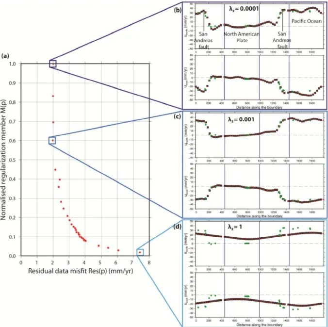
At first, we attempt to evaluate the Tikhonov parameter . To do so, we analyse the trade-off 413
between the normalized regularization member of the functional along the domain 414
boundaries, , and the residual data misfit at all geodetic 415
measurements within the domain (Fig. 7a). Each point of the curve represents an optimization 416
for a given value of the regularization parameter . A decrease of corresponds to an 417
increase of the regularization of the velocity field along the domain boundary, meaning that 418
high gradient changes of are smoothed. This would confer some degree of smoothness to 419
the solution. On the contrary, a reduction of regularization enables a better fit to high velocity 420
gradient changes along the domain boundary. These particularly occur at the transition 421
between highly deforming fault zones and rigid far fields. Nevertheless, this may induce 422
undesirable velocity gradient variations where the velocity field is smooth. Hence, in order to 423
find the appropriate balance between the regularity of the boundary conditions and velocity 424
residual, we compare observed and modelled velocity distributions along the boundary (Fig. 425
7b-c-d). When the damping parameter is small (Fig. 7b), we allow the regularization term of 426
the functional to be high. This in turn permits to better fit the observed velocities close to the 427
boundaries and consequently within the domain. Nevertheless, the boundary solution may 428
show in some places a degree of sharpness that is not supported by any data. Increasing the 429
damping parameter used in Fig. 7c increases the regularity of the boundary conditions while 430
still fitting properly the data along the border. We observe that this is done without 431
significantly altering the fit between modelled and observed velocities. Finally, increasing the 432
damping parameter, which means that extremely smooth boundary conditions become 433
admissible, leads to incompatibility between modelled and observed velocities along the 434
border (Fig. 7d). From this analysis, we set the regularization parameter to for which 435
the balance between the regularization of the boundary conditions and the fit to observed 436
velocities within the domain appears to be optimal. 437
5.3 Results of the inversion 438
Considering the model geometry and parametrization previously described, we perform the 439
inversion of the GPS velocities for the two selected zones (Zone 1 and Zone 2) of the Western 440
United States. 441
5.3.1 Estimated relative rigidity and corresponding uncertainty distributions 442
The inversion of the interseismic velocities leads to the distribution of effective rigidity 443
illustrated by Fig. 8a-b. In the case of Zone 1 (Fig. 8a), the lowest values of (1-1.5) are 444
centered on the Mojave Desert, whereas slightly higher rigidities (1.5-4) are observed along 445
the San Andreas Fault system and in the extreme South of the Eastern California Shear Zone. 446
However, lower values of rigidity (associated with higher deformation rates) are expected 447
along the San Andreas Fault system rather than in the Mojave Desert. We expect that this 448
artefact is likely due to an over-correction of the post-seismic motion of the seismic events of 449
1992 (Landers), 1994 (Northridge) and 1999 (Hector Mine) within the CMM3 velocity field 450
(Liu et al., 2015) . When the GPS data are processed to only keep the interseismic velocity, 451
the post-seismic answer of the earthquakes is estimated at its best. This artefact in our results 452
could help identify the residual post-seismic motion left in the data. As for the high rigidities 453
(>12), they are associated to the South Basin and Range and the South Sierra Nevada where 454
no significant deformation needs to be accommodated. As an extension of Zone 1, the 455
inversion in Zone 2 (Fig. 8b) produces similar rigidity distribution along the SAF and the 456
extreme South of the ECSZ (1.5-4), with, again a surprisingly low rigidity (<1.5) in the 457
Mojave Desert. However, one main difference can be underlined as a zone with rigidity 458
ranging from 6 to 12 is found in the eastern part of the South Basin and Range. 459
As described in paragraph 3.4, we determine the uncertainties associated with our rigidity 460
estimation which essentially result both from the local measurement density and the 461
uncertainties associated with the data themselves. For each mesh element, we estimate the 462
lower and upper admissible value for rigidity (Fig. 9a-b). First, along all the active fault 463
systems, identified rigidity values are quite low as the amplitude between the upper and lower 464
bounds are lower than 3. The reliability of our solution in deforming zones comes from the 465
local high density of measurements and from large amplitude of the deformation. Conversely, 466
when entering rigid zones, where only few measurements are available, the uncertainties 467
increase very much reaching values that typically range from 2.5 to above 16 by several 468
orders of magnitude. This is notably the case East of the ECSZ. Although the distribution of 469
rigidity shown in Fig. 8a suggests an optimal value of 6-12, uncertainties in this area (Fig. 9) 470
indicate that a much larger rigidity value (higher than 16 by several orders of magnitude) is 471
also valid. This can be noted in the inversion over the shifted domain (Fig. 8b). 472
5.3.2 Associated residual velocities 473
Alongside with the distribution of the rigidity, we evaluate the difference between GPS and 474
the modelled velocities to produce the residual map (Fig. 10a-b). The fit between observed 475
and modelled data is estimated using the normalized root mean square ( ) (McCaffrey, 476
2005), 477
(20) where and stand for the eastern and northern directions respectively, is the residual 478
velocity, the data standard error and N the number of data. In addition to the , the 479
weighted root mean square ( ) gives a measure of the a posteriori weighted scatter in 480
the fits (McCaffrey, 2005), 481
(21) For Zone 1 (Fig. 10a), we get a of 1.26, with a of 1.10 mm/yr that can be 482
compared with the uncertainty of 1.20 mm/yr associated with the data. The highest residuals 483
(>4.5 mm/yr) occur on the southern segments of the SAF, while intermediate residuals (2.5-484
4.5 mm/yr) are unevenly distributed between high and low data density zones. 485
A similar analysis for Zone 2 gives a of 1.25 (Fig. 10b) with a of 0.93 mm/yr. 486
The difference observed in the values of both zones can be explained by the data distribution. 487
Indeed, the second zone excludes some of the velocities that are poorly estimated by the 488
optimization (notably on the Pacific plate) and includes few vectors that are better recovered. 489
490
6. DISCUSSION 491
Based on the hypothesis that interseismic strain mostly reflects rheological contrasts across 492
the lithosphere, the solved inverse problem entirely depends on the quality of the CMM3 493
velocity field. Therefore, we first discuss the sensitivity of the model result with respect to the 494
data. Then, we discuss our results (strain rate and rigidity distributions) in the light of the ones 495
provided by previous studies on western US and California. We finally discuss the future use 496
of our method for tectonic and geodynamic purposes. 497
6.1 Robustness of the inversion 498
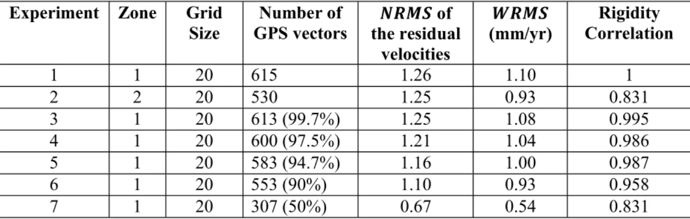
In this study, we use the entire dataset of the Southern California Crustal Motion Map Version 499
3.0, involving 615 vectors for Zone 1 and 530 vectors for Zone 2. In order to evaluate the 500
impact of data selection on rigidity distribution, we perform complementary inversions using 501
identical parametrization, but removing GPS vectors whose residual norms are greater than 502
a given threshold value. These residuals can be due to three different factors: 503
1) GPS uncertainty. Data uncertainties range from 0.16 mm/yr to 3.71 mm/yr for the 504
horizontal components with a value of 1.20 mm/yr. The maximum data 505
uncertainties are observed in the South of Mojave Desert, along the Los Angeles Bay 506
and for a few isolated points in the Sierra Nevada and ECSZ. 507
2) Local motions. Besides interseismic plate motions, some sites may be affected by 508
gravitational collapse, geothermal activity (e.g. Vasco et al., 2002) or the exploitation 509
of aquifer systems (e.g. Galloway et al., 1998; Hoffmann et al., 2001). Many different 510
processes can locally obscure the GPS interseismic velocity component, such as 511
unravelled postseismic motions. 512
3) Modelling. The optimization algorithm and the forward model can also be at the 513
origin of the residual velocities. Indeed, a poor estimation of the velocity along the 514
boundaries could be the reason why high residual velocities are observed at the 515
junction between the fault and the boundaries of the domain for both synthetic and real 516
data cases. Furthermore, our forward model includes several assumptions such as an 517
absence of body forces. Also, the data are assumed free of post-seismic effects which 518
can be inexact if all post-seismic effects due to the Landers, Northridge and Hector 519
Mine earthquakes, for instance, have not been fully removed. 520
We choose to withdraw from 0.3% ( 6 mm/yr) up to 50% ( 1.3 mm/yr) of the data in 521
order to analyse the stability of the solution of our inversion. The corresponding , 522
and the correlation of the rigidity distribution with respect to the one obtained by the 523
previously described inversion are gathered in Error! Reference source not found.. We 524
choose experiment 1 as the reference solution to estimate the rigidity correlation. Removing 525
up to 10% of the GPS measurements exhibiting significant residuals in our initial inversion 526
(experiences 3 to 6 in Table 1) neither enhance the or the , nor significantly 527
modify the rigidity distribution. But considering only 50% of the data (experience 7 in Table 528
1) improves the to 0.67 and the to 0.54 mm/yr and leads to a rigidity 529
correlation of 0.831 with the main features preserved. 530
This approach echoes the strategy Meade and Hager (2005) developed to reduce the number 531
of stations and therefore to minimize the uncertainty magnitude. While based on different 532
quality criteria, they remove about 50% of the initial dataset (CMM3) to compute their 533
inversions. Our results illustrate that selecting the data with the lowest residuals does not 534
significantly influence the modelled rigidity (see correlation in Table 1). However, in areas 535
where data density is poor, a reduction of 50% can lead to a completely different 536
interpretation. Therefore, keeping the whole dataset seems preferable. 537
6.2 Strain rate: comparison with other approaches 538
Most of strain rate computations derived from GPS velocity measurements stand on a 539
continuous approximation of a model velocity field. A simple way to compute the strain rate 540
is to design a triangulation of the GPS points collection and then assume that the velocity field 541
inside each triangle evolves linearly. However, this method generates a non-smooth strain 542
map due to a linear interpolation of measured GPS velocities. This method can be adapted to 543
areas covered by sparse GPS networks (Masson et al., 2005) but generates erroneous strain 544
rates when applied to dense networks such as the ones installed in California. In this case, a 545
smooth approximation of the velocity field needs to be performed in order to avoid spurious 546
strain rate modeling. Consequently, a suitable method must also account for high strain 547
gradient occurring around fault zones. A large variety of mathematical approaches can be 548
used to deduce a strain rate map, often leading to relatively large differences (Feigl et al., 549
1993; Mc Caffrey et al., 2005; Shen et al., 1996; Tape et al., 2009). 550
Our optimal solution of rigidity distribution can be used for the determination of strain rates 551
over the whole study area. But, we have shown above that our models systematically 552
underestimate rigidity in very few deforming areas, typically far from the active fault systems. 553
This bias is partly counterbalanced by the information provided by the upper bound of the 554
admissible rigidity values. These latter are very close to the optimal solution in deforming 555
zones, while they suggest that a purely rigid behavior may be considered when the 556
deformation is very small, even though a slight deformation remains admissible just 557
considering geodetic measurements 558
way to conform to geological considerations and block-model assumptions that state that, in 559
most cases, far from the faults, the blocks are rigid. So, we used the upper bound rigidity 560
distribution (Fig. 9b) for creating our strain rate map (Fig. 11a). 561
We compare in Fig. 11 our strain rate map (through the 2nd invariant of the strain tensor) with
562
the one obtained by a method originally proposed by Haines and Holt (1993) and later revised 563
in the framework of the strain map global project (Kreemer et al., 2014). Although both 564
methods depend on distinct assumptions, they produce similar intensities (> 64 nanostrain/yr) 565
located near faulted areas along the SAF and the ECSZ. This overall similarity is probably 566
due to the fact that both approaches are able to produce a low residual between the discrete 567
and the continuous velocity fields. Using our strongest admissible rigidity solution leads to 568
low strain estimates in weakly deforming areas that are similar to the ones obtained by the 569
global strain map project. This can be noticed in the Great Valley between the SAF and the 570
Sierra Nevada and along the Pacific coast. 571
A significant difference between the two strain rate maps can be found only on two limited 572
areas: offshore the Pacific coast and east of the ECSZ. Because these two areas display low 573
residuals (Fig. 10), we guess that our model is likely not able to locally estimate the strain rate 574
precisely. This could be due on the one hand, to an improper estimate of the boundary 575
conditions notably within the Pacific plate, and on the other hand, to a very low local data 576
density. Indeed, whereas Kreemer et al. (2014) only interpolate the strain rate dataset to best 577
fit the data, our solution aims at doing the same, but under the constraint of the stress 578
equilibrium equation (Eq. 1). As demonstrated by the synthetic benchmarks presented in 579
paragraph 3.4, evenly distributed data lead to a better estimation of the rigidity. Therefore, a 580
future use of our methodology could be to invert interpolated GPS velocities (such as the ones 581
provided by the Global Strain Rate Project) instead of the original GPS data to compute 582
effective rigidity distribution at a continental scale. 583
Lastly, we compare the spatial distribution of our dilatational strain rate solution with the one 584
obtained by Kreemer et al. (2014) (Fig. 12). We use the first invariant of the strain rate tensor 585
(mean of its trace) as a first-order approximation of the dilatational strain rate. 586
Neither the strain compatibility approach used by Kreemer et al. (2014) nor our study, take 587
vertical velocity measurements into account. Nevertheless, the plane stress formalism of our 588
modelling leads to the prediction of vertical strain rates, which is not the case in Kreemer et 589
al. (2014) analysis. Yet, recent analyses (e.g., Becker et al., 2015) suggest that the rate-change 590
of vertical loading of the lithosphere may play a dominant role in defining the distributions of 591
seismicity and therefore strain. 592
Despite the difference in their estimation, both spatial distributions of the dilatation strain rate 593
from Kreemer et al. (2014) and us are very similar. They notably highlight the compressive 594
context of the SAF system along the central bend. The only noticeable difference can be 595
found along the fault system located north of Los Angeles where vertical motion is known to 596
occur along active thrust faults (e.g. Northridge or Compton faults). 597
6.3 Rigidity of the lithosphere and effective elastic thickness 598
In the following, we study the relation between in-plane rigidity associated with geodetic 599
strain (this work) and the flexural rigidity deduced from gravity and topographic data analysis 600
(Audet and Bürgmann, 2011; Lowry and Pérez-Gussinyé, 2011; Tesauro et al., 2011). In the 601
case of a thin curved elastic plate, the relation between the bending moment and the 602
flexural rigidity is given by: 603
(22) where is the vertical displacement of the plate and R(x) its local curvature radius 604
(e.g.Turcotte and Schubert, 2002). Using Eq. 2, a horizontal force per unit area applied to a 605
vertical section of the lithosphere can be defined as: 606
(23) where is the stiffness of the lithosphere to horizontal strain. is equal to where is 607
the shear modulus (Pa) and the plate thickness (m). Therefore, in-plane rigidity is 608
expressed in N while the flexural rigidity is given in Nm, precluding a direct comparison 609
between these two fields. In order to compare our relative rigidity map with the flexural 610
rigidity deduced from gravity and topographic data analysis (Audet and Bürgmann, 2011; 611
Lowry and Pérez-Gussinyé, 2011; Tesauro et al., 2011), we use the elastic thickness 612
associated to these two formalisms. 613
The study of Lowry and Pérez-Gussinyé (2011) provides a map of the flexural elastic 614
thickness ( ) for the entire western US. We assume that a linear relationship exists between 615
the in-plane plate rigidity and its corresponding thickness (Chery, 2008 and present work). 616
Therefore, our map of is directly proportional to the distribution of shown in Fig. 8a. 617
Although such a linear relationship is valid only if elastic parameters do not vary with depth, 618
it provides a simple way to estimate the effective elastic thickness for our modelling. For the 619
purpose of comparison with Lowry and Pérez-Gussinyé (2011), we display their value of 620
over Zone 1 (Fig. 13). Flexural and geodetic elastic thicknesses displayed in Fig. 13 show a 621
very limited degree of agreement. For example, the flexural thickness map predicts a thick 622
plate for most of the SAF, while a low geodetic elastic thickness is deduced using the 623
interseismic velocity field. The only area suggesting some resemblance corresponds to the 624
Basin and Range around the ECSZ and the SAF around the Salton Trough for which both 625
methods display low elastic thickness. In order to find some justifications about the large 626
discrepancies between and at least two lines of arguments could be investigated. 627
First, despite the formal similarity between flexural plate and shear plate theories (Chéry et 628
al., 2011), they may reflect two distinct lithospheric behaviours. For example, as stated by 629
Thatcher and Pollitz (2008), plate flexure is the result of a long term loading over millions of 630
years, implying that the strain rate in most of the lithosphere is close to zero. is a measure 631
of stress that is supported dynamically over very long timescales by a lithosphere that is in a 632
state of frictional failure and viscoelastic flow, meaning the strain rate is virtually zero. 633
However, given the shorter timescale of geodetic observation and the clear evidence for 634
seismic release of significant elastic strain potential accumulated on century timescales, 635
likely does predominantly reflects the elastic behavior of a thicker domain associated to 636
interseismic deformation. Another difference may come from the lithospheric loading. 637
Vertical loads modify distinct components of the strain tensor. Indeed, those induce flexure 638
and plate motions and therefore horizontal shear. Hence, distinct behaviours may emerge 639
from these kinds of load. 640
In the brittle part of the crust, background seismicity is likely to reflect the loading of 641
interseismic motion, therefore introducing an anelastic component into the analysed shear 642
motion. Beneath the crust and especially under a shear zone like the San Andreas Fault 643
system, the upper mantle presents a laterally variable and strong anisotropy (Hartog and 644
Schwartz, 2001). If such anisotropic behaviours occur at both crustal and mantle levels, 645
flexural and horizontal loading may activate two different rheological systems that could 646
result into significant differences in terms of effective elastic thickness. 647
A second way to investigate is to assume that flexural and geodetic thicknesses represent the 648
same mechanical concept. However, they could be differently revealed by the data because of 649
the formal differences between the two inverse problems. In the case of flexural thickness, the 650
determination of is based on the correlation between topographic and gravimetric signal. 651
Among other factors, erosion can smooth or sharpen the topographic signal. Even if its 652
influence can be accounted for in modelling approaches (e.g. Forsyth, 1985), the impact of 653
erosion on the determination of seems difficult to quantify due to large uncertainty 654
associated to past erosion. In addition, a geodynamical setting mostly involving shear motion 655
may not be adapted at all for a flexural plate analysis because such a motion is not likely to 656
produce neither topographic nor gravimetric signals. Last but not least, inverse theory of plate 657
flexure requires that flexural thickness cannot be determined for resolutions smaller than the 658
characteristic flexural wavelength (Watts, 2001). This also may explain why a sharp rigidity 659
variation across the SAF cannot be resolved by this method. Even if our methodology has 660
never been used prior to Chéry et al. (2001), the direct relation between shear strain and shear 661
rigidity is likely to produce high resolution estimate of geodetic thickness for zones where the 662
geodetic strain is well defined. Conversely, we acknowledge that our uncertainty analysis 663
predicts inaccurate rigidity determination in zones of low strain-rate like the Sierra Nevada. 664
Also, lithospheric loads like body forces and basal stress coming from mantle motion can 665
impact the strain-rate field and therefore altering the determination of the shear rigidity. The 666
identification of the importance of such effects must be tackled by future studies. 667
In order to better understand the discrepancy between flexural and shear analysis, a tractable 668
way would be to design a complete mechanical model of western US as it was done for 669
example by Pollitz et al. (2010). Such a model could be used to predict synthetic topographic, 670
gravimetric and deformation datasets obeying to momentum and constitutive equations. Then 671
672
lithospheric deformation and compared to the rheological input of the forward model. 673
674
7. CONCLUSION 675
A global inversion strategy has been proposed for the identification of effective rigidity maps 676
using GPS velocity fields under minimum a priori assumptions. Taking advantage of the self-677
adjoint nature of the governing equations, large dimensional problems coming from necessary 678
high resolution distribution of the rigidity have been considered. Compared to the previous 679
study carried out by Chéry et al. (2011), the results are now backed by uncertainty analysis 680
which suggests that the effective rigidity can only be accurately determined in moderate or 681
highly strained areas. 682
This is a high-resolution methodology which can be seen as a mechanical model to link shear 683
rigidity to interseismic strain with no prior knowledge of fault locations. The main limitation 684
of this approach relies to the plane stress hypothesis used in the forward model. Therefore, no 685
strain variation occurs with depth for a given horizontal location over the plate. This 686
behaviour is probably over simplified around active faults acting like screw dislocations as 687
proposed by Savage and Burford (1973). To complete what is presented here, the following 688
directions can be considered: 689
1) The 2D effective rigidity model can be replaced by a 3D model of Western United 690
States including the effective elastic thickness as the main geophysical parameter. 691
Because this approach would include the full 3D strain rate tensor, it would provide a 692
more realistic approximation of the plate behaviour of the lithosphere especially 693
around faults. 694
2) The 2D approach can be used over wide areas, for instance at the continental plate 695
scale, after a splitting in patches. This would permit to determine large scale rigidity 696
maps in the framework of the global strain map project of (Kreemer et al., 2014). 697
3) The strong spatial correlation between low rigidity areas and active fault zones also 698
suggests that our methodology could be applied for deciphering active faults in 699
tectonically poorly known areas. 700
701
ACKNOWLEDGEMENTS 702
We thank Prof. Riad Hassani from Nice-Sophia Antipolis University for making available to 703
us his plane stress Finite Element code CAMEF. We also acknowledge Tony Lowry and an 704
anonymous reviewer for their constructive remarks and suggestions. The PhD of S. Furst is 705
supported by the Total Company and the LabEx NUMEV project (n° ANR-10-LABX-20) 706
fund 707
French National Research Agency (ANR). 708
BIBLIOGRAPHY 710
Allaire, G., Jouve, F., Toader, A.M., 2004. Structural optimization using sensitivity analysis 711
and a level-set method. J. Comput. Phys. 194, 363 393. doi:10.1016/j.jcp.2003.09.032 712
Anderson, K., Segall, P., 2013. Bayesian inversion of data from effusive volcanic eruptions 713
using physics-based models: Application to Mount St. Helens 2004-2008. J. Geophys. 714
Res. Solid Earth 118, 2017 2037. doi:10.1002/jgrb.50169 715
Audet, P., Bürgmann, R., 2011. Dominant role of tectonic inheritance in supercontinent 716
cycles. Nat. Geosci. 4, 184 187. doi:10.1038/ngeo1080 717
Becker, T.W., Lowry, A.R., Faccenna, C., Schmandt, B., Borsa, A., Yu, C., 2015. Western 718
US intermountain seismicity caused by changes in upper mantle flow. Nature 524, 458 719
461. doi:10.1038/nature14867 720
Bird, P., Kong, X., 1994. Computer simulations of California tectonics confirm very low 721
strength of major faults. Geol. Soc. Am. Bull. doi:10.1130/0016-722
7606(1994)106<0159:CSOCTC>2.3.CO;2 723
Chéry, J., 2008. Geodetic strain across the San Andreas fault reflects elastic plate thickness 724
variations (rather than fault slip rate). Earth Planet. Sci. Lett. 269, 351 364. 725
doi:10.1016/j.epsl.2008.01.046 726
Chéry, J., Mohammadi, B., Peyret, M., Joulain, C., 2011. Plate rigidity inversion in southern 727
California using interseismic GPS velocity field. Geophys. J. Int. 187, 783 796. 728
doi:10.1111/j.1365-246X.2011.05192.x 729
Chéry, J., Zoback, M.D., Hassani, R., 2001. An integrated mechanical model of the San 730
Andreas Fault in central and northern California. J. Geophys. Res. 106, 22051. 731
doi:10.1029/2001JB000382 732
Dzurisin, D., 2003. A comprehensive approach to monitoring volcano deformation as a 733
window on the eruption cycle. Rev. Geophys. 41, 1001. doi:10.1029/2001RG000107 734
Feigl, K.L., Agnew, C., Dong, D., Hager, H., Herring, A., Jackson, D.D., Jordan, T.H., King, 735
W., Larson, M., Murray, M.H., Webb, F.H., 1993. Space Geodetic Measurement of 736
Crustal Deformation in Central and Southern California , 1984-1992. J. Geophys. Res. 737
98, 1984 1992. 738
Forsyth, W., 1985. Subsurface Loading and Estimates of the Flexural Rigidity of Continental 739
Lithosphere. J. Geophys. Res. 90, 12623 12632. 740
Galloway, D.L., Hudnut, K.W., Ingebritsen, S.E., Phillips, S.P., Peltzer, G., Rogez, F., Rosen, 741
P. a., 1998. Detection of aquifer system compaction and land subsidence using 742
interferometric synthetic aperture radar, Antelope Valley, Mojave Desert, California. 743
Water Resour. Res. 34, 2573. doi:10.1029/98WR01285 744
Haines, A.J., Holt, W.E., 1993. A Procedure for Obtaining the Complete Horizontal Motions 745
Within Zones Deformation of Strain Rate Data. J. Geophys. Res. 98, 12057 12082. 746
doi:10.1029/93jb00892 747
Hartog, R., Schwartz, S.Y., 2001. Depth-dependent mantle anisotropy below the San Andreas 748
fault system: Apparent splitting parameters and waveforms. J. Geophys. Res. 106, 4155. 749
doi:10.1029/2000JB900382 750
Hesse, M. a., Stadler, G., 2014. Joint inversion in coupled quasi-static poroelasticity. J. 751
Geophys. Res. Solid Earth 119, 1425 1445. doi:10.1002/2013JB010272 752
Hoffmann, J., Zebker, H.A., Galloway, D.L., Amelung, F., 2001. Seasonal subsidence and 753
rebound in Las Vegas Valley, Nevada, observed by synthetic aperture radar 754
interferometry. Water Resour. Res. 37, 1551 1566. doi:10.1029/2000WR900404 755
Ivorra, B., Mohammadi, B., Ramos, A.M., 2013. Design of code division multiple access 756
filters based on sampled fiber Bragg grating by using global optimization algorithms. 757
Optim. Eng. 1 19. doi:10.1007/s11081-013-9212-z 758
Kreemer, C., Hammond, W.C., 2007. Geodetic constraints on areal changes in the Pacific 759