Characterization of Polar Stratospheric Clouds with Space-Borne Lidar: CALIPSO and the 2006 Antarctic Season

(1)

HAL Id: hal-00302855

https://hal.archives-ouvertes.fr/hal-00302855

Submitted on 5 Jun 2007

HAL is a multi-disciplinary open access

archive for the deposit and dissemination of sci-entific research documents, whether they are pub-lished or not. The documents may come from teaching and research institutions in France or abroad, or from public or private research centers.

L’archive ouverte pluridisciplinaire HAL, est destinée au dépôt et à la diffusion de documents scientifiques de niveau recherche, publiés ou non, émanant des établissements d’enseignement et de recherche français ou étrangers, des laboratoires publics ou privés.

Characterization of Polar Stratospheric Clouds with

Space-Borne Lidar: CALIPSO and the 2006 Antarctic

Season

M. C. Pitts, L. W. Thomason, L. R. Poole, D. M. Winker

To cite this version:

M. C. Pitts, L. W. Thomason, L. R. Poole, D. M. Winker. Characterization of Polar Stratospheric Clouds with Space-Borne Lidar: CALIPSO and the 2006 Antarctic Season. Atmospheric Chemistry and Physics Discussions, European Geosciences Union, 2007, 7 (3), pp.7933-7985. �hal-00302855�

(2)

ACPD

7, 7933–7985, 2007 Characterization of Antarctic PSCs with CALIPSO M. C. Pitts et al. Title Page Abstract Introduction Conclusions References Tables Figures ◭ ◮ ◭ ◮ Back Close Full Screen / Esc

Printer-friendly Version Interactive Discussion

EGU Atmos. Chem. Phys. Discuss., 7, 7933–7985, 2007

www.atmos-chem-phys-discuss.net/7/7933/2007/ © Author(s) 2007. This work is licensed

under a Creative Commons License.

Atmospheric Chemistry and Physics Discussions

Characterization of Polar Stratospheric

Clouds with Space-Borne Lidar: CALIPSO

and the 2006 Antarctic Season

M. C. Pitts1, L. W. Thomason1, L. R. Poole2, and D. M. Winker1

1

NASA Langley Research Center, Hampton, VA, USA

2

Science Systems and Applications, Incorporated, Hampton, VA, USA Received: 4 May 2007 – Accepted: 25 May 2007 – Published: 5 June 2007 Correspondence to: M. C. Pitts (michael.c.pitts@nasa.gov)

(3)

ACPD

EGU

Abstract

The role of polar stratospheric clouds in polar ozone loss has been well documented. The CALIPSO satellite mission offers a new opportunity to characterize PSCs on spa-tial and temporal scales previously impossible. A PSC detection algorithm based on a single wavelength threshold approach has been developed for CALIPSO. The method

5

appears to accurately detect PSCs of all opacities, including tenuous clouds, with a very low rate of false positives and few missed clouds. We applied the algorithm to CALIOP data acquired during the 2006 Antarctic winter season from 13 June through 31 October. The spatial and temporal distribution of CALIPSO PSC observations is il-lustrated with weekly maps of PSC occurrence. The evolution of the 2006 PSC season

10

is depicted by time series of daily PSC frequency as a function of altitude. Comparisons with “virtual” solar occultation data indicate that CALIPSO provides a different view of the PSC season than attained with previous solar occultation satellites. Measurement-based time series of PSC areal coverage and vertically-integrated PSC volume are computed from the CALIOP data. The observed area covered with PSCs is significantly

15

smaller than would be inferred from the commonly used temperature-based proxy TNAT but is similar in magnitude to that inferred from T_STS. The potential of CALIOP mea-surements for investigating PSC composition is illustrated using combinations of lidar backscatter and volume depolarization for two CALIPSO PSC scenes.

1 Introduction

20

Extensive measurements and modeling activity over the past two decades have firmly established that polar stratospheric clouds (PSCs) play an essential part in the spring-time chemical depletion of ozone at high latitudes (Solomon, 1999). The role of PSCs is twofold. First of all, PSC particles serve as catalytic sites for heterogeneous chem-ical reactions that transform stable chlorine and bromine reservoir species into highly

25

(4)

ACPD

EGU sediment, they can irreversibly redistribute gaseous odd nitrogen (a process commonly

known as denitrification), thereby slowing the reformation of the chlorine reservoirs and exacerbating the ozone depletion process. In spite of the recent progress made in understanding PSCs and their chemical effects, there are still significant gaps in our knowledge, primarily in the areas of solid particle formation and their denitrification

5

potential. These uncertainties limit our ability to accurately represent PSCs in global models and call into question the accuracy of PSC predictions for a future stratosphere whose composition will differ from the current state. This is of particular concern in the Arctic, where winter temperatures hover near the PSC threshold and, hence, future stratospheric cooling could lead to enhanced cloud formation and substantially greater

10

ozone losses.

Much of our present understanding of PSCs is based on remote sensing observa-tions. Long-term solar occultation data records from the Stratospheric Aerosol Mea-surement (SAM) II (Poole and Pitts, 1994) and Polar Ozone and Aerosol MeaMea-surement (POAM) II and III (Fromm et al., 1997; Fromm et al., 1999; Fromm et al., 2003)

in-15

struments have established the general climatology of PSCs such as their occurrence at very cold temperatures (T <195–200 K) and their spatial distribution and seasonal variability in both the Arctic and Antarctic. Measurements from polarization sensitive airborne and ground-based lidar systems have also made valuable contributions to our understanding of PSCs. In particular, lidar observations have established that

20

there are three primary forms of PSC particles: supercooled liquid ternary (H2SO4 -HNO3-H2O) solution droplets (STS) that evolve from background aerosol without a phase change; solid nitric acid hydrate crystals, most likely nitric acid trihydrate (NAT); and H2O ice (Poole and McCormick, 1988; Browell et al., 1990; Toon et al., 1990). Multi-year ground-based lidar observations have been utilized to study the seasonal

25

chronology of PSC composition (David et al., 1998; Gobbi et al., 1998; Santacesaria et al. 2001; Adriani et al., 2004). More recently, satellite limb emission measurements of the infrared spectra of PSCs by the Michelson Interferometer for Passive Atmo-spheric Sounding (MIPAS) instrument on ENVISAT have provided valuable new insight

(5)

ACPD

EGU to PSC composition (e.g. Spang et al., 2005; H ¨opfner et al., 2006). Solar occultation

and ground-based and airborne lidar data, however, have inherent shortcomings that limit a more comprehensive understanding of PSC processes. For instance, solar oc-cultation measurements have very coarse spatial resolution (hundred of kilometers), are limited to 14–15 profiles per day in each hemisphere, and only occur at the

day-5

night terminator. Ground-based lidar records are of course from single locations and are often interrupted by optically thick tropospheric clouds, while airborne lidar PSC data records are both short-term and limited to relatively localized along-track spatial coverage.

Spaceborne lidar measurements are particularly well-suited for probing PSCs and

10

may provide a more comprehensive picture of clouds than attainable with these existing PSC remote sensing data sources. The Lidar-In-space Technology Experiment (LITE) demonstrated the potential of space lidar for observation of clouds and aerosol (Winker et al., 1996). The Geoscience Laser Altimeter System (GLAS), launched aboard the Ice Cloud and land Elevation Satellite (ICESat) in 2003, measures atmospheric

15

backscatter profiles at two wavelengths (532 and 1064 nm) and has observed PSCs (Palm et al., 2005). However, this system is not polarization sensitive, and due to laser lifetime concerns, the observational periods are restricted to three 33-day campaigns per year and 532-nm profile data are limited (Abshire et al., 2005). The Cloud-Aerosol-Lidar and Infrared Pathfinder Satellite Observations (CALIPSO) mission, launched on

20

28 April 2006, provides a unique set of measurements to study PSCs. The CALIPSO PSC data record will have much higher vertical and spatial resolution than solar occul-tation data, but more importantly, the CALIPSO data are collected continuously along the orbit track so that PSC information will be extracted in the polar night region and not solely at the terminator. Similar to many airborne and ground-based systems, the

25

CALIPSO backscatter data are recorded in two orthogonal polarization channels at 532 nm, and in a third channel at 1064 nm. This combination of measurements pro-vided by CALIPSO offers promise of additional information on microphysical properties, particularly the presence of large solid particles in mixed-phase clouds, a crucial

(6)

ele-ACPD

EGU ment for understanding and accurate prediction of the role that PSCs play in polar

ozone loss, but without interference from tropospheric clouds and the limits in spatial and temporal coverage of ground-based and airborne lidar data records.

In this paper, we describe an algorithm to detect polar stratospheric clouds in the CALIPSO data. We then apply the algorithm to CALIPSO data from the 2006 Antarctic

5

winter season to demonstrate the robustness of the approach and highlight the unique capabilities of CALIPSO for characterizing PSCs.

2 CALIPSO description

The CALIPSO mission is designed to provide global, vertically resolved measurements of clouds and aerosols to improve our understanding of their role in climate forcing

10

(Winker et al., 2003). The CALIPSO instrument payload consists of the Cloud-Aerosol Lidar with Orthogonal Polarization (CALIOP), the Infrared Imaging Radiometer (IIR), and the Wide Field Camera (WFC). CALIOP is a two-wavelength, polarization sensi-tive lidar that provides high vertical resolution profiles of backscatter coefficient at 532 and 1064 nm, as well as two orthogonal (parallel and perpendicular) polarization

com-15

ponents at 532 nm (Winker et al., 20071). Table 1 provides a summary of the CALIOP instrument parameters. Although the fundamental sampling resolution of CALIOP is 30 m in the vertical and 333 m in the horizontal, an altitude-dependent on-board av-eraging scheme is employed that provides highest resolution in the troposphere and lower resolution in the stratosphere. The resultant downlink resolution of the CALIOP

20

data is listed in Table 2. A detailed discussion of the CALIOP data products can be found in Vaughan et al. (2004).

CALIPSO is in a 98◦ _{inclination orbit with an altitude of 705 km and is a part of} the Aqua satellite constellation that includes the Aqua, CloudSat, Aura, and

PARA-1

Winker, D. M., McGill, M., and Hunt, W. H.: Initial performance assessment of CALIOP, Geophys. Res. Lett., in review, 2007.

(7)

ACPD

EGU SOL platforms. Although PSC studies are not one of its primary mission objectives,

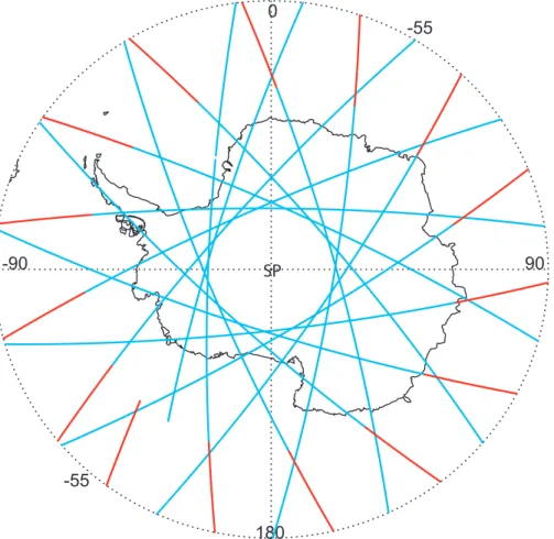
CALIPSO is an ideal platform for studying polar processes since its orbit provides ex-tensive measurement coverage over the polar regions of both hemispheres with an average of fourteen orbits per day extending to 82◦ _{latitude. Figure 1 illustrates the} measurement coverage over the Antarctic for a single day (28 June 2006) with blue

5

points representing the nighttime measurement locations and red points representing the daytime measurement locations. On average, over 300 000 lidar profiles are ac-quired per day at latitudes poleward of 55◦_{, providing a unique dataset for studying the} occurrence, composition, and evolution of PSCs. In contrast, SAM II made less than 60 000 observations over the Antarctic during the entire eleven year period from 1978

10

to 1989.

3 PSC detection algorithm

The PSC detection algorithm is an automated process to identify PSCs in the CALIOP Level 1B Data Product. In the initial version described herein, we have adopted a single wavelength threshold approach using the CALIOP 532-nm backscatter

coeffi-15

cient measurements although we anticipate future versions will also incorporate the CALIOP 532-nm depolarization and 1064-nm backscatter coefficient measurements. All results shown in this paper are based on Version 1.10 of the CALIPSO data prod-uct available publicly through the NASA Langley Atmospheric Science Data Center (http://eosweb.larc.nasa.gov/).

20

For this initial PSC detection algorithm, we restricted our analysis to CALIOP night-time measurements only. While PSCs can be seen in the daynight-time data, the daynight-time measurements have higher background signals due to scattered sunlight. This forces the use of a significantly higher PSC detection threshold for the CALIOP daytime mea-surements than for the nighttime meamea-surements. We will consider the use of daytime

25

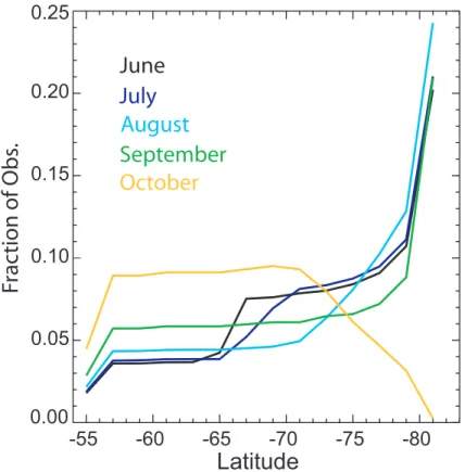
measurements in the future. Figure 2 shows the distribution of the nighttime measure-ment locations as a function of latitude for each month of the PSC season. As expected

(8)

ACPD

EGU for CALIPSO’s orbit inclination of 98◦_{, during most of the season there is a sharp}

maxi-mum in the number of measurements at the crossover point of the orbit near 82◦_{S with} the remainder of the measurements more evenly distributed in latitude. By October, the Sun is illuminating a larger portion of the polar region and the majority of nighttime measurement locations are distributed between about 55◦ _{and 75}◦_{S. The latitudinal}

5

distribution of nighttime measurement locations will be taken into consideration when we examine the statistics of PSC occurrence over the Antarctic region as a whole.

3.1 Data preparation

The standard CALIOP Level 1B data files contain a half orbit (day or night) of cali-brated and geolocated full resolution profiles of attenuated backscatter coefficient at

10

532 and 1064 nm and perpendicular attenuated backscatter coefficient at 532 nm. In addition, the Level 1B files contain profiles of meteorological data that are also com-ponents of the detection algorithm. This data is derived from the Goddard EOS Data Assimilation System (GEOS-4) products (Bloom et al., 2005; Lin, 2004) interpolated to the CALIPSO measurement locations.

15

The altitude region of interest for PSC detection ranges from near the tropopause up to about 30 km and spans several CALIOP spatial resolution regimes (see Table 2). Specifically, the resolution of the Level 1B CALIOP data is 60-m vertical and 1-km horizontal for altitudes between 8.2 km and 20.2 km and 180-m vertical and 1.67-km horizontal for altitudes between 20.2 km and 30 km. This change in averaging scales

20

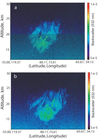
produces a distinct difference in the noise characteristics of the data across the 20.2-km boundary as illustrated in Fig. 3a. In addition to having finer spatial resolution, the data below 20.2 km also exhibit a significantly larger range in background noise. Since the cloud detection algorithm is based on ensemble statistics, mixing data with significantly different noise characteristics would produce unpredictable results. One solution would

25

be to treat the two altitude regimes separately for cloud detection, but this would add significant complexity to the algorithm and it is possible that the two methods would give different results and create an artificial boundary in the PSC analyses. Instead,

(9)

ACPD

EGU we applied additional spatial averaging to all data below 20.2 km to closely match the

resolution of the data above 20.2 km. The additional averaging produces a dataset with consistent resolution and noise characteristics over the entire altitude range of interest as shown in Fig. 3b. The change in spatial scales and the concomitant change in noise character at the 8.2, 20.2, 30.1 km boundaries are sometimes visible in the CALIPSO

5

lidar Level 1B browse images (available at:http://www-calipso.larc.nasa.gov/products/ lidar/).

Since the lower bound for PSC opacity merges into the background aerosol, we have chosen to perform additional averaging of the data to reduce the noise levels in the data and lower the detection limit for PSCs. Some of this noise occurs in the form of

10

radiation induced noise spikes. Although these events are typically isolated, they occur with sufficient frequency that their inclusion in our analyses would produce systematic bias in the ensemble statistics and false positive cloud detection. We found that first applying a 5-km horizontal median filter eliminates the majority of these noise spikes while only modestly impacting the spatial resolution. To further reduce the noise, we

15

also averaged the data to 540-m resolution in the vertical.

We applied the additional processing described above to the Level 1B CALIOP data to produce an input dataset for the cloud detection algorithm that has single profile resolution of 540-m vertical and 5-km horizontal. To reduce the data volume, we limited our analyses to latitudes poleward of 55◦_{S and to altitudes between 10 and 30 km.}

20

3.2 Algorithm description

The CALIPSO PSC detection algorithm is similar to the traditional single wavelength extinction threshold techniques used in solar occultation PSC identification schemes such as Poole and Pitts (1994) and Fromm et al. (2003). In these previous studies, PSCs were identified as those measurements having extinction coefficients

signifi-25

cantly larger than the background (non-PSC) aerosol extinction. Instead of extinction, the CALIPSO cloud detection algorithm is based on measurements of scattering ratio

(10)

ACPD

Printer-friendly Version Interactive Discussion EGU at 532 nm, R(532), defined as R_{(532) =} βT(532) β_m(532) (1)

where β_m(532) is the volume molecular backscatter coefficient at 532 nm and βT(532) is the total (molecular + aerosol) volume backscatter coefficient at 532 nm. βm(532) is calculated from the GEOS-4 molecular number density profiles provided in the CALIOP

5

Level 1B data files and a theoretical value for the molecular scattering cross section as described in Hostetler et al. (2006). βT(532) is derived directly from the attenuated backscatter coefficient at 532 nm reported in the CALIOP Level 1B data files by ap-plying a first-order correction for molecular and ozone attenuation based on GEOS-4 molecular and ozone number density profiles provided in the CALIOP Level 1B data

10

files.

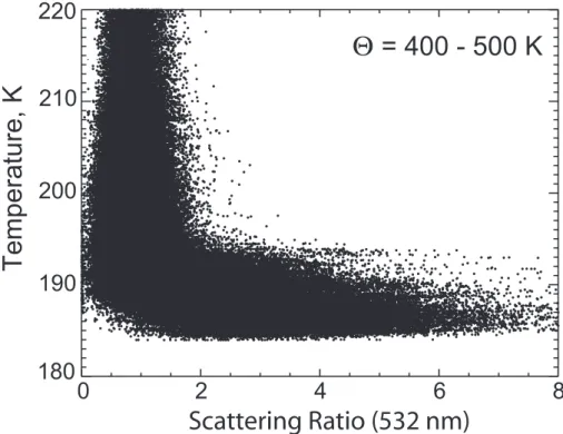
Figure 4 shows an ensemble of CALIOP scattering ratio measurements as a function of observed temperature from 13 June 2006 over the Southern polar region. Within the winter polar vortex, the background aerosol population is characterized by very low optical depth values (Thomason and Poole, 1993) and is represented in Fig. 4 by the

15

nearly vertical family of points with scattering ratio values close to 1. The spread of the background aerosol data is representative of the magnitude of the noise in the measurements (σ=0.32) at these spatial scales (540-m vertical ×5-km horizontal) and is consistent with the observed CALIOP nighttime signal-to-noise ratio in the strato-sphere. The statistics of the data totally change below about 195 K where the upper

20

limit of the scattering ratio values increases dramatically from ∼2 to ∼8. In Fig. 4, the enhanced scattering ratio values in excess of ∼2 observed at cold temperatures roughly correspond to the PSC visible in Fig. 3. This characteristic dependence of PSC occurrence on cold temperature is the physical basis for our detection algorithm. It allows us to characterize the statistics of the background aerosol data at warmer

25

temperatures apart from the presence of PSCs. PSCs are then identified as statistical outliers in terms of scattering ratio from the background aerosol ensemble occurring at temperatures below a pre-selected threshold temperature, T_PSC. The background

(11)

ACPD

EGU aerosol population is characterized by the ensemble of points that occur at

tempera-tures warmer than T_PSC, with the assumption that the optical properties of the back-ground aerosol are not significantly dependent on temperature. Based on the distribu-tion of the background aerosol populadistribu-tion, a scattering ratio threshold, RPSC, is defined such that a large fraction of the warm temperature points lie below this value. Points

5

that exceed this value and are below TPSCare considered to be PSCs. The ensemble statistics and corresponding PSC scattering ratio threshold, RT, are computed on a complete day of nighttime CALIOP observations, then PSCs are identified on a profile-by-profile basis.

The algorithm is summarized by the following steps:

10

1. The background aerosol population is defined as the ensemble of scattering ratio points with temperatures above TPSC=198 K.

2. RT is defined as the scattering ratio value corresponding to the 99.5 percentile (∼2.6σ) of the background aerosol population defined in step (1).

3. PSCs are identified as those points with temperature below TPSCand scattering

15

ratio values exceeding RT.

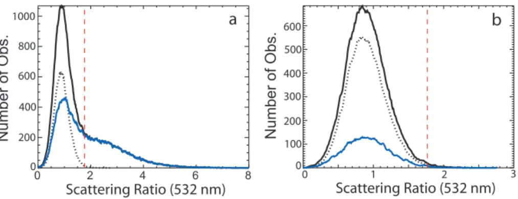
The detection process is illustrated graphically in Fig. 5a for the same ensemble of scattering ratio points as shown in Fig. 4. The scattering ratio distribution for the en-tire ensemble is represented by the solid black line and is characterized by a roughly Gaussian-shaped core corresponding to the background aerosol and a long positive

20

tail corresponding to the PSCs. The background aerosol distribution alone, defined by all points with T >TPSC, is depicted by the black dotted line and is nearly Gaussian shaped with no positive tail and a mode scattering ratio nearly identical to that of the en-tire ensemble. The dashed red line indicates the value of R_T corresponding to the 99.5 percentile of the background aerosol distribution alone. The 99.5 percentile value was

25

chosen as the PSC threshold based on trial and error. The sensitivity of the detection algorithm to both R_T and T_PSCare discussed in Sect. 3.3. The blue line represents the

(12)

ACPD

EGU distribution of ensemble points with T <TPSC, which includes both background aerosol

and PSCs. There is a peak in the cold (blue) distribution corresponding to the back-ground aerosol at cold temperatures and a pronounced positive tail corresponding to the PSCs. The slight positive shift of the mode scattering ratio of the cold background points (blue line) is suggestive of growth of the entire aerosol population as the

temper-5

ature cools. This may be a slight violation of our basic assumption that the ensemble optical properties of the background aerosol are not significantly dependent on tem-perature. However the shift is small and we are forced to live with this behavior. By definition, all points in the cold (blue) distribution with scattering ratios larger than RT are identified as PSCs. For contrast, the corresponding ensemble distribution curves

10

for a day in late October with no PSCs present are shown in Fig. 5b. In the absence of PSCs, all three curves are representative of the background aerosol distribution and have similar near-Gaussian shapes with no positive tails.

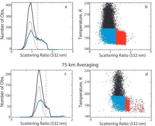
As is evident from Fig. 4, PSCs with scattering ratios greater than about 2 are easy to discriminate from the background aerosol population. However, optically thin PSCs

15

with backscatter ratios less than about 2 are more difficult to detect above the measure-ment noise present in the 5-km resolution backscatter data. To enhance the detection of these more tenuous PSCs, two additional passes are made through the data with 25-km and 75-km horizontal averaging applied to the data. Each successive level of increased spatial averaging reduces the noise level in the data, exposing the more

ten-20

uous PSCs. Figure 6 illustrates the effect of the successive averaging on the ensemble distributions and scatter plots. Compared with Figs. 4 and 5a, each level of additional smoothing reduces the spread in the data, lowering the scattering ratio threshold for PSC detection. On average, RT has a value of near 1.8 for the 5-km resolution data; 25-km averaging reduces RT to about 1.3; and 75-km smoothing further reduces RT

25

to values near 1.2. Using this successive averaging approach, the threshold for PSC detection is decreased by almost a factor of four.

(13)

ACPD

EGU 3.3 PSC detection sensitivity

The detection algorithm is empirical by nature and the selection of values for RT and

T_PSC is not clear cut. Since the value of T_PSCdefines the ensemble of scattering ratio points used to characterize the optical properties of the background aerosol popula-tion, the most important criterion for selecting TPSC is to choose a value sufficiently

5

large to exclude PSCs from the background aerosol ensemble. We chose a value of

T_{P SC}_{=198 K. This value is warm enough to exclude most if not all clouds from the}

back-ground ensemble. We found that changing TPSC by +1–2◦ changes the total number of PSCs identified by about 1%. However, dropping the PSC temperature threshold to 196 K clearly allows some PSC values to be included in the background aerosol

10

ensemble. As a result, this raises the PSC scattering ratio threshold and decreases the number of PSCs identified by as much as 6%. It is crucial to set the threshold temperature large enough to exclude most if not all PSCs while not setting it so large that the sample size becomes too small. We have found that 198 K is sufficient in all cases. The identification of PSCs is also sensitive to the percentile value selected for

15

the scattering ratio threshold. We considered using the 97.5 percentile (∼2σ) and the 99.85 percentile (∼3σ), as well as, the 99.5 percentile value as the scattering ratio threshold. Visual inspection of the data revealed that using the 97.5 percentile pro-duced a large number of false positives. These appeared in the images as isolated PSC “pixels” highly indicative of noise rather than the coherent structure of a

geophys-20

ical object. On the other hand, the 99.85 percentile results were similar to the 99.5 percentile, but reduced the overall size of the sample to the point that determining the threshold RT value became noisy and highly variable with time. Therefore, we find that the 99.5 percentile definition is robust in the sense that it produces few false positives and allows a sample size sufficiently large to produce robust statistics.

25

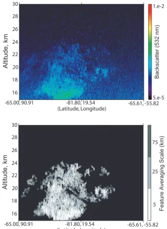
Two examples are shown to illustrate the performance of the PSC detection algo-rithm. The top panel of Fig. 7 shows the CALIOP 532-nm backscatter coefficient data from a single orbit on 15 June 2006. The corresponding PSC mask produced from the

(14)

ACPD

EGU PSC detection algorithm is shown in the bottom panel of Fig. 7. The averaging scale

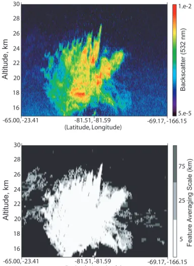
(5-, 25-, or 75-km) at which the PSC was detected is indicated by the shading. For this optically-thin PSC case, the detection algorithm is able to discriminate even the thinnest parts of the cloud from the background signal, although higher levels of spatial averaging are required to detect the more tenuous regions above the noise. Figure 8

5

shows a similar comparison for an optically thick PSC case from 24 July 2006. As ex-pected, the optically-thick PSCs are easily identified by the detection algorithm during the first pass at the 5-km resolution. It is noteworthy that the cloud edges are accu-rately reproduced and the tenuous clouds surrounding the dense cloud are also being detected during subsequent passes at larger spatial scales. Based on visual

inspec-10

tion of dozens of images similar to those shown in Figs. 7 and 8, the CALIPSO PSC detection algorithm appears to be working exceptionally well. Based on the frequency of random, isolated PSC points, the rate of false positives is extremely low, 0.1% or less. Missed clouds are more difficult to quantify, but following visual inspection of a number of images we did not observe any features likely to be PSCs that weren’t

iden-15

tified as such. At the lower end of the scale, PSC scattering ratio merges into that of the background aerosol. While higher levels of smoothing capture much of this behav-ior, we are, by definition, missing some segment of this low backscatter continuum. In addition, PSCs that are characterized by very low particle number densities such as a NAT “haze” may not produce detectable enhancements in backscatter coefficient and

20

could therefore also be missed in this initial version of the algorithm. Future versions will attempt to reduce this aerosol-PSC ambiguity by incorporating the additional 1064-nm backscatter coefficient and polarization information available in the CALIPSO data products. For instance, inclusion of the 532-nm perpendicular backscatter coefficient data may allow us to detect thin layers of NAT haze.

(15)

ACPD

EGU

4 2006 Antarctic PSC season

As a test of the PSC detection algorithm, we examined the CALIPSO PSC observa-tions during the 2006 Antarctic season. We applied the PSC detection algorithm to all CALIPSO data from 13 June (first date available) until 31 October 2006. To quantify the occurrence of PSCs spatially, we defined a 21×21-box grid in polar stereographic

5

coordinates centered on the South Pole and extending to 55◦_{S at its sides. Each of} the 441 grid boxes covers an area approximately 350 km×350 km. For a selected time interval such as a day or week, a PSC frequency is defined for each grid box as the ratio of the number of PSCs observations to the total number of CALIPSO observations within that box. Later, we will utilize this PSC frequency as roughly the equivalent to

10

areal coverage of PSCs within a grid box. The resolution of the grid was chosen as a compromise between the need for adequate sampling within each grid box and the desire to retain high spatial resolution. This is more of an issue for the low latitude boxes. For example, in a typical week, the grid boxes at high latitudes have nearly two thousand CALIOP observations, while grid boxes at lower latitudes near the edge of

15

the grid have several hundred observations.

4.1 Seasonal evolution

The meteorological conditions in the Antarctic stratospheric during the 2006 winter set the stage for a record ozone hole in terms of both area and ozone mass deficit (Gutro, 2006; WMO Bulletin, 2007). Temperatures poleward of 50◦_{S at 50 mb were colder}

20

than the 1979–2005 average from early August through November. During this same time period, the area of the polar vortex at 450 K was significantly larger than average. This led to a much larger than average ozone hole and, in fact, during many days in November the ozone hole area was larger than had been observed at any time between 1979 and 2005 (WMO Bulletin, 2007). In addition, the ozone mass deficit was higher

25

than for any year since 1997 (WMO Bulletin, 2007). Since CALIPSO began routine data acquisition on 13 June, the initial onset of PSCs was not observed by CALIPSO

(16)

ACPD

EGU in 2006.

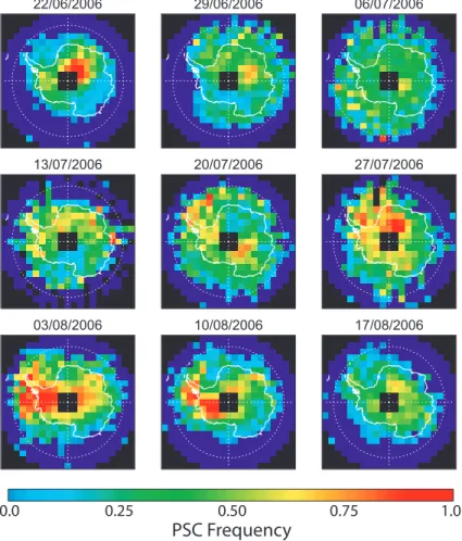
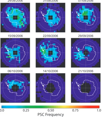
To examine the spatial distribution of PSCs over the course of the 2006 Antarctic win-ter, weekly PSC frequency maps were produced for every 540 m in altitude between 10 and 30 km. Examples from two altitudes are shown in Figs. 9 and 10. At 20 km (Fig. 9), PSCs were prevalent over a large fraction of the polar region from the onset of the

5

CALIPSO measurements in mid-June until mid-August, after which PSCs significantly diminished and eventually disappeared by mid-October. At 15 km (Fig. 10), PSCs were less widespread early in the season than at 20 km, but became ubiquitous over the po-lar region by July and persisted well into October. At all altitudes, PSCs were commonly observed over most of the Antarctic continent, but their frequency rapidly diminished

10

away from the continent at lower latitudes. Although the location of the maximum PSC frequency tended to vary from week to week, there were clearly some preferred regions for PSC occurrence. This is evident in Fig. 11, where we show the longitudinal distribu-tion of PSCs as a funcdistribu-tion of altitude. PSCs were observed over all longitudes, but the two favored regions for PSC occurrence were over the ice sheets of East Antarctica

15

and over the Antarctic Peninsula near 90◦_{W where the PSC frequency occasionally} exceeded 60%. The longitudinal distribution of temperature (from GEOS-4) confirms that the longitudinal distribution of PSCs is strongly correlated with cold temperatures as shown by Poole and Pitts (1994).

To examine the temporal evolution of PSCs for the Antarctic as a whole, we produced

20

daily time series of PSC frequency as a function of altitude. In this context, the PSC frequency represents the cumulative sum over the entire grid of the PSC frequency (areal coverage) within each grid box on a given day at a given altitude. To account for both the uneven latitudinal sampling (see Fig. 2) and the tendency for PSCs to occur more frequently at higher latitudes, the PSC frequencies are weighted by their

loca-25

tion in either the inner core or outer fringe of the grid. The inner core consists of the central 11×11 grid boxes and the outer fringe contains all remaining grid boxes. The calculated PSC statistics for these two regions are given weights proportional to their relative areal size: 121/441 for the inner core and 320/441 for the outer fringe. The

(17)

ACPD

EGU CALIPSO time series of daily PSC frequency is shown in Fig. 12a and the

correspond-ing daily-averaged GEOS-4 temperature at the CALIPSO measurement locations is shown in Fig. 12b. A maximum PSC frequency of slightly less than 0.30 (interpreted as 30% of the grid was covered with PSCs) occurred during several periods between the end of June and mid-August. By early September, PSC frequency had diminished

5

significantly at all altitudes. Then in mid-September, PSC activity increased again for a few weeks before tapering off in October. The altitude of the peak PSC occurrence slowly decreased from near 22 km in June to below 15 km by September and October. As expected, the maximum PSC frequency is highly correlated with region of coldest temperatures.

10

4.2 Comparison with solar occultation PSC climatologies

Much of our current knowledge of PSC occurrence over the Antarctic has been based on the historical records of solar occultation satellite instruments such as SAM II (1978– 1993) and POAM II/II data (1996–2006) (e.g. Poole and Pitts, 1994; Fromm et al., 1997; Nedoluha et al., 2003). A significant limitation of solar occultation climatologies is that

15

they are representative of only the temporally varying latitudes at which the occulta-tion observaocculta-tions are being made and not of the entire polar region, especially the polar night which is never sampled by the solar instruments. In general, solar occul-tation measurement latitudes for sun-synchronous platforms like POAM III and SAM II vary slowly (nominally 1◦_–2◦_{per week) with season, reaching highest (lowest) latitudes}

20

near the equinoxes (solstices). Solar occultation instruments will generally saturate when observing optically thick PSCs and, hence, this class of clouds is not included in their data records. In contrast, no saturation is apparent in any of the CALIPSO PSC images. With these limitations, there have been questions regarding how generally representative these solar occultation climatologies are. With CALIPSO’s high-density

25

spatial sampling, it is straightforward to mimic solar occultation sampling and produce “solar occultation”-like time series of PSC frequency. Using SAM II measurement lat-itudes as the reference for solar occultation, we produced a time series of daily PSC

(18)

ACPD

EGU frequency using only CALIPSO measurements from the latitude band that would have

been observed by SAM II. This virtual “solar occultation” PSC frequency time series is shown in Fig. 13a. Compared to the Poole and Pitts (1994) climatology for the Antarctic, the virtual “solar occultation” time series is similar with peak frequency occurring below 16 km in September. In fact, the 2006 season is very similar to the cold 1987 season

5

statistics shown in Poole and Pitts (1994). This is quite different than the CALIPSO time series (Fig. 12) where with the peak PSC frequency occurs much earlier near the be-ginning of August and higher in altitude near 20 km. We also constructed a virtual “solar occultation” time series representing the POAM II/III measurement latitudes, but both instruments sampled at higher latitudes in September than observed by CALIPSO so a

10

complete POAM-like time series was not possible. The virtual POAM solar occultation time series (excluding September) is similar to the evolution observed by POAM II/III as shown in Fromm et al. (1997) and Nedoluha et al. (2003) with peak PSC frequency observed later in the season than observed with CALIPSO. Considering the solar oc-cultation sampling pattern, it is no surprise that their observed maximum in PSC

fre-15

quency occurs in September since that is when the occultation measurement locations are near their highest latitude and the observed temperatures are coldest (Fig. 13b). In light of the differences between the CALIPSO and virtual “solar occultation” PSC statistics, it is clear that in 2006, at least, the temporal distribution of solar occultation PSC observations would not be representative of the Southern polar region as a whole.

20

4.3 PSC processing diagnostics

Chemical ozone loss in the polar regions is strongly related to the geographical extent of PSCs during the winter (e.g. Rex et al., 1999, 2004, 2006; Tilmes et al., 2004). To date, realistic measurement-based estimates of PSC areal coverage have not been feasible due in large part to the limited sampling pattern of solar occultation

instru-25

ments. Instead, proxies for total PSC area have been developed based on ture. The most frequently used proxy for PSC areal extent is the area with tempera-ture less than TNAT calculated from global temperature analyses such as ECMWF or

(19)

ACPD

EGU GEOS-4 and an assumption of thermodynamic equilibrium with NAT, the most stable

phase of PSCs that occur at temperatures above the water frost point (Hanson and Mauersberger, 1988). However, with the extensive measurement coverage afforded by CALIPSO, observational-based estimates of the geographical extent of PSCs are now possible. The daily PSC frequency (Fig. 12a) easily scales into total PSC areal

cover-5

age as a function of altitude and is shown in Fig. 14. By early July, PSCs are covering over 10 million km2at altitudes between about 20–23 km. The region of maximum PSC area expands in size into early August when PSCs are covering over 10 million km2 at altitudes between about 15 and 23 km. The total volume of atmosphere encompassed by PSCs can be determined by vertical integration of the PSC area and is shown in

10

the bottom panel of Fig. 14. The PSC volume generally increases from mid-June un-til it reaches a peak of near 150 million km3 on about 1 August, after which it steadily decreases until 1 September. There is a slight increase in PSC volume during the last two weeks of September, corresponding to the brief upturn in PSC frequency at that time, after which PSC volume continues to decrease until it reaches zero by the end of

15

October.

The CALIPSO-based estimates of PSC areal coverage provide a means to evaluate the robustness of temperature proxies for PSC formation such as TNAT. We used the formulation of Hanson and Mauersberger (1988) along with profiles of HNO3and H2O mixing ratio from the EOS (Aura) Microwave Limb Sounder (MLS) (Data Version 1.5)

20

(Froidevaux et al., 2006) to produce maps of TNAT. To account for the large spatial and temporal variations in the observed HNO3and H2O mixing ratios, we produced daily-averaged, zonal mean profiles of HNO₃and H₂O mixing ratio for 5◦_{latitude bands from} 55◦_{S to 85}◦_{S. Figures 15 and 16 show sample time series of Aura MLS zonal HNO}

3 mixing ratio, H2O mixing ratio, and the derived TNAT for the 5◦latitude bands centered at

25

67.5◦_{S and 82.5}◦_{S. During the 2006 winter, Aura MLS observed very low HNO}

3mixing ratios (<2 ppbv) and H2O mixing ratios (<3 ppmv) over a large area within the polar vor-tex. At 82.5◦_{S, significant denitrification and dehydration had occurred by mid-winter} and, as a result, T_NAT was below 190 K over a large altitude region during much of

(20)

Au-ACPD

EGU gust and September. At 67.5◦_{S, the onset of denitrification was delayed and not nearly}

as severe as what occurred at higher latitudes and the corresponding TNAT was greater than 190 K over most of the stratosphere. Using the MLS-derived zonal mean profiles of T_NAT, an estimate of the area with T <T_NATwas produced in an analogous fashion as the CALIPSO PSC area by calculating the cumulative sum over the entire grid of the

5

fraction of occurrence within each grid box of GEOS-4 temperatures less than TNAT. The result is shown in Fig. 17. Qualitatively, the temporal and spatial evolution of the area with T <TNAT is similar to the observed CALIPSO PSC area, but its magnitude is larger than the CALIPSO PSC area by almost a factor of two. The accuracy of the TNAT area calculations are dependent on the accuracy of the GEOS-4 temperature and MLS

10

gas species mixing ratio data, but it is unlikely these uncertainties are large enough to explain the observed discrepancy. It is also possible that the CALIPSO PSC areal extent is being underestimated since a subset of optically-thin PSCs such as NAT haze may not be detected in this version of the algorithm.

An alternative proxy for PSC occurrence is the equilibrium temperature of STS, TSTS.

15

We produced an estimate of the area with T <T_STS (shown in Fig. 18) where we have assumed that TSTS is 4 K colder than TNAT (Tabazadeh et al., 1994). While there are still differences, the evolution of the area with T <TSTS agrees much better with the CALIPSO PSC area and is nearly identical in magnitude. Therefore, for the 2006 Antarctic winter, there is much better agreement between the observed CALIPSO PSC

20

area and TSTS than TNAT. This is in approximate agreement with Santee et al. (1998) who showed strong correspondence between the area of T <192 K and the area of gas-phase HNO3 loss, an indicator of PSC formation, but weak correspondence between the area of T <195 K and the area of gas-phase HNO3loss. The CALIPSO-based PSC areas will provide an opportunity to further investigate the accuracy of these proxies

25

(21)

ACPD

EGU 4.4 PSC composition studies

Although not a primary goal of this work, the CALIPSO lidar measurements are also well-suited for probing the composition of PSCs. The CALIOP backscatter data are recorded in two orthogonal polarization channels at 532 nm, and in a third channel at 1064 nm. This combination of data provides crucial information of PSC particle size

5

(through changes in absolute backscatter and its wavelength dependence) and phase (via the 532-nm perpendicular backscatter). For instance, the presence of large non-spherical particles in sufficient quantities will produce changes in the ensemble optical properties such as the ratio of 1064-nm to the 532-nm backscatter (color ratio) and especially the 532-nm depolarization ratio. For illustrative purposes, we show a few

10

examples of how the CALIPSO data may be exploited to infer PSC composition. In a follow-up paper (Poole et al., 2007), we explore the information content of the CALIOP data with regard to PSC composition in detail.

In Fig. 19 is shown a scatter diagram of CALIOP scattering ratio at 532 nm versus volume depolarization at 532 nm for measurements identified as PSCs on a single orbit

15

from 24 July 2006. A commonly used scheme for optical classification of PSC remote sensing observations has evolved from analyses of polarization sensitive lidar data (Poole and McCormick, 1988; Browell et al., 1990; Toon et al., 1990): type 1a for NAT, type 1b for STS, and type 2 for H₂O ice. More recent studies by Toon et al. (2000) and Biele et al. (2001) have shown that such “typing” of PSC data is somewhat of an

20

oversimplification, with the clouds often being mixtures of solid and liquid particles in reality. For illustrative purpose, we subset the CALIPSO PSC data into three groups (STS, H2O ice, and mixtures of STS, H2O ice, and NAT) based on the combinations of backscatter ratio and volume depolarization as shown in Table 3. The CALIPSO measurements roughly corresponding to STS (red) and H₂O ice (blue) are indicated in

25

the figure. All other points are considered mixtures. Figure 20 shows two examples of PSC composition inferred from the CALIPSO measurements. The image in Fig. 20a corresponds to the tenuous PSC shown in Fig. 7. Based on this simple classification

(22)

ACPD

EGU scheme, the PSC consists almost exclusively of STS droplets. The image in Fig. 20b

corresponds to the intense PSC event shown in Fig. 8. In this case, the cloud consists of a large H2O ice core that is surrounded by mixtures of particles. Near the bottom right edge of the cloud, a region of mostly STS is observed. This particular PSC occurred near the Antarctic Peninsula and is likely a mountain-wave induced cloud.

5

Although we have used a simplistic analysis in these examples, it is clear that the CALIPSO data offers promise of additional information on PSC physical properties.

5 Summary and conclusions

The CALIPSO mission provides a unique dataset for studying the formation, evolution, and composition of PSCs. The CALIPSO PSC data record has higher vertical and

spa-10

tial resolution than previously attainable from spaceborne remote sensors and extends into the polar night region. As the first step in exploiting this promising database, we have developed an automated algorithm to detect PSCs in the CALIPSO Level 1B data. The detection approach is based on CALIOP scattering ratio measurements at 532 nm and uses a single threshold in scattering ratio for PSC identification. Successive levels

15

of smoothing are applied to the data to increase the sensitivity for detecting optically thin PSCs. Based on visual inspection of dozens of CALIPSO PSC cloud images, the detection algorithm is robust with only a small fraction of false positives and few if any missed clouds that were apparent in the backscatter data.

As a test of the algorithm, we examined CALIPSO PSC observations from the 2006

20

Antarctic winter (13 June until 31 October). With its extensive measurement coverage in the polar regions, CALIPSO provides a comprehensive view of the spatial and tem-poral distribution of PSCs during the Antarctic winter. CALIPSO observed widespread PSCs over much of the Antarctic region from June through August, after which PSCs significantly diminished, except for a brief resurgence in the latter half of September,

25

and eventually disappeared by mid-October. Throughout the season, PSCs were most frequently observed over East Antarctica and near the Antarctic Peninsula, where at

(23)

ACPD

EGU times the PSC frequency exceeded 60%. Comparison of the CALIPSO PSC statistics

with virtual “solar occultation” data indicates that solar occultation PSC statistics would not be representative of the Antarctic region as a whole during the 2006 winter. Al-though this is not surprising given their inherent sampling limitations, it is a reminder that the historical solar occultation-based PSC climatologies are strictly representative

5

of their sampling latitudes and not of the polar region as a whole. The solar occultation climatologies should be re-evaluated in the context of what we learn from CALIPSO.

Measurement-based estimates of PSC area and volume were derived from the CALIPSO PSC observations. The CALIPSO PSC area is about a factor of two smaller than the area with T <T_NAT, a commonly used proxy to predict PSC occurrence. The

10

CALIPSO PSC area may be underestimated since optically-thin PSCs such as NAT haze may not be detected in this initial version of the algorithm, but it’s not clear how much these would contribute to the overall area. Future versions of the detection al-gorithm will include polarization measurements to aid in identification of this class of PSC. The CALIPSO PSC area is similar in magnitude to the area encompassed by

15

T <T_STS. Further study is required to understand the implications of this finding and to

understand whether T_STSis a better proxy for PSC formation in the Antarctic than T_NAT or whether the process is too complex for a single parameter proxy to capture. In any case, it is clear that CALIPSO measurements offer a unique opportunity to investigate PSC proxies and ultimately develop improved predictors of PSC occurrence.

20

The potential of the CALIPSO data for PSC composition studies was demonstrated. Three crude PSC compositions were defined based on combinations of 532-nm scat-tering ratio and volume depolarization ratio measurements. CALIPSO data can clearly be utilized for discrimination of STS and H2O ice PSCs. Perhaps a more important question is the composition of the mixed phase clouds. A more in-depth examination

25

of the PSC microphysical information imbedded in the CALIPSO data is forthcoming (Poole et al., 2007). Correlative studies combining CALIPSO and MIPAS PSC obser-vations may provide a more comprehensive picture of PSC microphysical properties, particularly the presence of large NAT particles in mixed-phase clouds.

(24)

ACPD

EGU

Acknowledgements. The Aura MLS data were provided courtesy of the MLS Team and ob-tained through the Aura MLS website (http://mls.jpl.nasa.gov/index-eos-mls.php).

References

Abshire, J. B., Sun, X., Riris, H., Sirota, J. M., McGarry, J. F., Palm, S., Yi, D., and Liiva, P.: Geoscience Laser Altimeter System (GLAS) on the ICESat Mission: On-orbit measurement 5

performance, Geophys. Res. Lett., 32, L21S02, doi:10.1029/2005GL024028, 2005.

Adriani, A., Massoli, P., Di Donfrancesco, G., Cairo, F., Moriconi, M. L., and Snels, M.: Cli-matology of polar stratospheric clouds based on lidar observations from 1993 to 2001 over McMurdo Station, Antarctic, J. Geophys. Res., 109, D24211, doi:10.1029/2004JD004800, 2004.

10

Biele, J., Tsias, A., Luo, B. P., Carslaw, K. S., Neuber, R., Beyerle, G., and Peter, T.: Nonequi-librium coexistence of solid and liquid particles in Arctic stratospheric clouds, J. Geophys. Res., 106, 22 991–23 007, 2001.

Bloom, S., da Silva, A., Dee, D., Bosilovich, M., Chern, J.-D., Pawson, S., Schubert, S., Sienkiewicz, M., Stajner, I., Tan, W.-W., and Wu, M.-L.: Documentation and Validation of 15

the Goddard Earth Observing System (GEOS) Data Assimilation System – Version 4, Tech-nical Report Series on Global Modeling and Data Assimilation 104606, 26, 2005.

Browell, E. V., Butler, C. F., Ismail, S., Robinette, P. A., Carter, A. F., Higdon, N. S., Toon, O. B., Schoeberl, M. R., and Tuck, A. F.: Airborne lidar observations in the wintertime Arctic stratosphere: polar stratospheric clouds, Geophys. Res. Lett., 17, 385–388, 1990.

20

David, C., Bekki, S., Godin, S., Megie, G., and Chipperfield, M. P.: Polar stratospheric clouds climatology over Dumont d’Urville between 1989 and 1993 and the influence of volcanic aerosols on their formation, J. Geophys. Res., 103, 22 163–22 180, 1998.

Froidevaux, L., Livesey, N. J., Read, W. G., Jiang, Y. B., et al.: Early validation analyses of atmospheric profiles from EOS MLS on the Aura Satellite, IEEE Transactions on Geoscience 25

and Remote Sensing, 44, 1106–1121, 2006.

Fromm, M. D., Lumpe, J. D., Bevilacqua, R. M., Shettle, E., Hornstein, J., Massie, S. T., Fricke, K. H.: Observations of Antarctic polar stratospheric clouds by POAM II: 1994–1996, J. Geo-phys. Res., 102, 23 659–23 672, 1997.

Fromm, M. D., Bevilacqua, R. M., Hornstein, J., Shettle, E., Hoppel, K., Lumpe, J. D.: An 30

(25)

ACPD

EGU

analysis of Polar Ozone and Aerosol Measurement (POAM) II Arctic polar stratospheric cloud observations, 1993–1996, J. Geophys. Res., 104, 24 341–24 357, 1999.

Fromm, M. D., Alfred, J. M., and Pitts, M.: A unified long-term, high-latitude strato-spheric aerosol and cloud database using SAM II, SAGE II, and POAM II/III data: Algo-rithm description, database definition and climatology, J. Geophys. Res., 108(D12), 4366, 5

doi:10.1029/2002JD002772, 2003.

Gobbi, G. P., Di Donfrancesco, G., Adriani, A.: Physical properties of stratospheric clouds during the Antarctic winter of 1995, J. Geophys. Res., 103, 10 859–10 873, 1998.

Gutro, R.: NASA and NOAA announce ozone hole is a double record breaker. (http://www.

nasa.gov/vision/earth/lookingatearth/ozone record.html), October 2006. 10

Hansen, D. R. and Mauersberger, K.: Laboratory studies of the nitric acid trihydrate: Implica-tions for the south polar stratosphere, Geophys. Res. Lett., 15, 855–858, 1988.

H ¨opfner, M., Luo, B. P., Massoli, P., Cairo, F., Spang, R., Snels, M., Di Donfrancesco, G., Stiller, G., von Clarmann, T., Fischer, H., and Biermann, U.: Spectroscopic evidence for NAT, STS, and ice in MIPAS infrared emission measurements of polar stratospheric clouds, Atmos. 15

Chem. Phys., 6, 1201–1219, 2006,

http://www.atmos-chem-phys.net/6/1201/2006/.

Hostetler, C. A., Liu, Z., Reagan, J., Vaughan, M., Winker, D., Osborn, M., Hunt, W. H., Powell, K. A., Trepte, C.: CALIOP Algorithm Theoretical Basis Document- Part 1: Calibration and Level 1 Data Products, PC-SCI-201, NASA Langley Research Center, Hampton, VA, (avail-20

able at:http://www-calipso.larc.nasa.gov/resources/project documentation.php), 2006. Lin, S. J.: A “Vertically Langrangian” finite-volume dynamical core for global models, Mon. Wea.

Rev., 132, 2293–2307, 2004.

Manney, G. L., Allen, D. R., Kruger, K., Naujokat, B., Santee, M., Sabutis, J., Pawson, S., Swin-bank, R., Randall, C., Simmons, A., and Long, C.: Diagnostic comparison of meteorological 25

analyses during the 2002 Antarctic winter, Mon. Wea. Rev., 133, 1261–1278, 2005.

Nedoluha, G. E., Bevilacqua, R. M., Fromm, M. D., Hoppel, K. W., and Allen, D. R.: POAM measurements of PSCs and water vapor in the 2002 Antarctic vortex, Geophys. Res. Lett., 30(15), 1796, doi:10.1029/2003GL017577, 2003.

Palm, S. P., Fromm, M., and Spinhirne, J.: Observations of Antarctic polar stratospheric 30

clouds by the Geoscience Laser Altimeter System (GLAS), Geophys. Res. Lett., 32, L22S04, doi:10.1029/2005GL023524.

(26)

ACPD

EGU

Geophys. Res., 93, 8423–8430, 1988.

Poole, L. R. and Pitts, M. C.: Polar stratospheric cloud climatology based on Stratospheric Aerosol Measurement II observations from 1978 to 1989, J. Geophys. Res., 99, 13 083– 13 089, 1994.

Rex, M., Von Der Gathen, P., Braathen, G. O., Harris, N. R. P., Reimer, E., Beck, A., Alfier, R., 5

Kruger-Carstennsen, R., Chippenfield, M., De Backer, H., Balis, D., O’Connor, F., Dier, H., Dorokhov, V., Fast, H., Gamma, A., Gil, M., Kyro, E., Litynska, Z., Mikkelsen, I. S., Molyneux, M., Murphy, G., Reid, S. J., Rummukainen, M., and Zerefos, C.: Chemical ozone loss in the Arctic winter 1994/95 as determined by the Match technique, J. Atmos. Chem., 32, 35–59, 1999.

10

Rex, M., Salawich, R. J., von der Gathen, P., Harris, N. R. P., Chipperfield, M. P., and Naujokat, B.: Arctic ozone loss and climate change, Geophys. Res. Lett., 31, L04116, doi:10.1029/2003GL018844, 2004.

Rex, M., Salawitch, R. J., Deckelmann, H., von der Gathen, P., et al.: Arctic winter 2005: Impli-cations for stratospheric ozone loss and climate change, Geophys. Res. Lett., 33, L23808, 15

doi:10.1029/2006GL026731, 2006.

Santacesaria, V., McKenzie, R., and Stefanutti, L.: A climatological study of polar stratospheric clouds (198–1997) from lidar measurements over Dumont d’Urville (Antarctica), Tellus B, 53, 306–321, 2001.

Solomon, S.: Stratospheric ozone depletion: A review of concepts and history, Rev. Geophys., 20

37, 275–316, 1999.

Spang, R., Remedios, J. J., Kramer, L. J., Poole, L. R., Fromm, M. D., and M ¨uller, M., Baum-garten, G., and Konopka, P.: Polar stratospheric cloud observations by MIPAS on ENVISAT: detection method, validation and analysis of the northern hemisphere winter 2002/2003, At-mos. Chem. Phys., 5, 679–692, 2005,

25

Tabazadeh, A., Turco, R. P., Drdla, K., and Jacobson, M. Z.: A study of Type I polar stratospheric cloud formation, Geophys. Res. Lett., 21(15), 1619–1622, 1994.

Thomason, L. W. and Poole, L. R., Use of stratospheric aerosol properties as diagnostics of Antarctic vortex processes, J. Geophys. Res., 98, 23 003–23 012, 1993.

30

Tilmes, S., M ¨uller, R., Grooß, J.-U., Russell III, J. M.: Ozone loss and chlorine activation in the Arctic winters 1991–2003 derived with the tracer-tracer correlations, Atmos. Chem. Phys., 4, 2181–2213, 2004,

(27)

ACPD

EGU

Toon, O. B., Browell, E. V., Kinne, S., and Jordan, J.: An analysis of lidar observations of polar stratospheric clouds, Geophys. Res. Lett., 17, 393–396, 1990.

Vaughan, M., Young, S., Winker, D., Powell, K., Omar, A., Liu, Z., Hu, Y., and Hostetler, C.: Fully automated analysis of space-based lidar data: An overview of the CALIPSO retrieval 5

algorithms and data products, Proc. SPIE, 5575, 16–30, 2004.

Winker, D. M., McCormick, M. P., and Couch, R.: An overview of LITE: NASA’s Lidar In-space Technology Experiment, Proc. IEEE 84, 164–180, 1996.

Winker, D. M., Pelon, J., and McCormick, M. P.: The CALIPSO Mission: Spaceborne lidar for observations of aerosols and clouds, in: Lidar Remote Sensing for Industry and Environmen-10

tal Monitoring III, Proc., SPIE, 4893, edited by: Singh, U. N., Itabe, T., and Lui, Z., pp. 1–11, SPIE, Bellingham, WA, 2003.

World Meteorological Organization, Antarctic Ozone Bulletin No. 7 (available through the Global Atmospheric Watch program web page at:http://www.wmo.ch/web/arep/ozone.html)2006.

(28)

ACPD

EGU Table 1. CALIOP Instrument Characteristics.

laser: Nd: YAG, diode-pumped, Q-switched, frequency doubled

wavelengths: 532 nm, 1064 nm

pulse energy: 110 mJoule/channel

repetition rate: 20.25 Hz

receiver telescope: 1.0 m diameter

polarization: 532 nm

footprint/FOV: 100 m/ 130 µrad

vertical resolution: 30–60 m horizontal resolution: 333 m linear dynamic range: 22 bits

(29)

ACPD

EGU Table 2. Spatial Resolution of CALIOP Level 1B Data Products.

Altitude Range (km) Horizontal 532-nm Vertical 1064-nm Vertical

Resolution (km) Resolution (m) Resolution (m)

30.1 to 40.0 5.0 300 ----

20.2 to 30.1 1.67 180 180

8.2 to 20.2 1.0 60 60

-0.5 to 8.2 0.33 30 60

(30)

ACPD

EGU Table 3. PSC composition definitions.

Composition Scattering Ratio Depolarization Ratio (%)

STS < 5 < 2 H2O Ice > 10 > 10

(31)

ACPD

Printer-friendly Version Interactive Discussion EGU -90 0 90 180 -55 -55 SP

Fig. 1. Typical CALIPSO measurement coverage over the Antarctic for a single day (28 June

2006). Blue points indicate nighttime orbit segments and red points indicate daytime orbit segments.

(32)

ACPD

Printer-friendly Version Interactive Discussion EGU

-55

-60

-65

-70

-75

-80

Latitude

0.00

0.05

0.10

0.15

0.20

0.25 June

July

August

September

October

Fr

ac

tion of Obs

.

Fig. 2. Latitudinal distribution of sampling from CALIPSO nighttime orbits for each month of the

(33)

ACPD

Printer-friendly Version Interactive Discussion EGU Altitude, km Backscatter (532 nm) b Altitude, km Backscatter (532 nm) a 30 25 20 15 30 25 20 15 -55.00, 119.37 -80.11, 73.61 -65.67, -34.13 -55.00, 119.37 -80.11, 73.61 -65.67, -34.13 (Latitude, Longitude) (Latitude, Longitude) 1.e-2 1.e-2 5.e-5 5.e-5

Fig. 3. Panel (a) shows CALIOP backscatter coefficient data from an individual orbit on 13

June 2006 at the standard Level 1B spatial resolution. Panel (b) shows the same data, but with additional smoothing applied to all data below 20.2 km to closely match resolution of data above 20.2 km.

(34)

ACPD

Printer-friendly Version Interactive Discussion EGU

0

2

4

6

8 Temperature, K

Scattering Ratio (532 nm)

220

210

200

190

180 Θ = 400 - 500 K

Fig. 4. Ensemble of 532-nm scattering ratio measurements as a function of observed

temper-ature for the 400–500 K potential tempertemper-ature layer from an individual orbit of CALIPSO data on 13 June 2006.

(35)

ACPD

Printer-friendly Version Interactive Discussion EGU 0 2 4 6 8 Number of Obs. Scattering Ratio (532 nm) 1000 800 600 400 200 0 Number of Obs. 600 500 400 300 200 100 0 Scattering Ratio (532 nm) 0 1 2 3 a b

Fig. 5. Ensemble distributions of scattering ratio for a single orbit of data from (a) 13 June and (b) 25 October. The black line represents the distribution for the entire ensemble; the dotted

line represents the distribution of the background aerosol alone; and the blue line represents the distribution of all points with temperature less than T_PSC. The dashed red line indicates the value of R_T.