HAL Id: hal-00295367
https://hal.archives-ouvertes.fr/hal-00295367
Submitted on 28 Nov 2003
HAL is a multi-disciplinary open access
archive for the deposit and dissemination of
sci-entific research documents, whether they are
pub-lished or not. The documents may come from
teaching and research institutions in France or
abroad, or from public or private research centers.
L’archive ouverte pluridisciplinaire HAL, est
destinée au dépôt et à la diffusion de documents
scientifiques de niveau recherche, publiés ou non,
émanant des établissements d’enseignement et de
recherche français ou étrangers, des laboratoires
publics ou privés.
Operational mapping of atmospheric nitrogen deposition
to the Baltic Sea
O. Hertel, C. Ambelas Skjøth, J. Brandt, J. H. Christensen, L. M. Frohn, J.
Frydendall
To cite this version:
O. Hertel, C. Ambelas Skjøth, J. Brandt, J. H. Christensen, L. M. Frohn, et al.. Operational mapping
of atmospheric nitrogen deposition to the Baltic Sea. Atmospheric Chemistry and Physics, European
Geosciences Union, 2003, 3 (6), pp.2083-2099. �hal-00295367�
www.atmos-chem-phys.org/acp/3/2083/
Atmospheric
Chemistry
and Physics
Operational mapping of atmospheric nitrogen deposition to the
Baltic Sea
O. Hertel, C. Ambelas Skjøth, J. Brandt, J. H. Christensen, L. M. Frohn, and J. Frydendall
National Environmental Research Institute, Department of Atmospheric Environment, P.O. Box 358, Frederiksborgvej 399, 4000 Roskilde, Denmark
Received: 17 October 2002 – Published in Atmos. Chem. Phys. Discuss.: 8 July 2003 Revised: 7 November 2003 – Accepted: 17 November 2003 – Published: 28 November 2003
Abstract. A new model system for mapping and forecast-ing nitrogen deposition to the Baltic Sea has been devel-oped. The system is based on the Lagrangian variable scale transport-chemistry model ACDEP (Atmospheric Chemistry and Deposition model), and aims at delivering deposition estimates to be used as input to marine ecosystem models. The system is tested by comparison of model results to mea-surements from monitoring stations around the Baltic Sea. The comparison shows that observed annual mean ambient air concentrations and wet depositions are well reproduced
by the model. Diurnal mean concentrations of NHx(sum of
NH3and NH+4) and NO2are fairly well reproduced, whereas
concentrations of total nitrate (sum of HNO3and NO−3) are
somewhat overestimated. Wet depositions of nitrate and
ammonia are fairly well described for annual mean values, whereas the discrepancy is high for the monthly mean values and the wet depositions are rather poorly described concern-ing the diurnal mean values. The model calculations show that the annual atmospheric nitrogen deposition has a pro-nounced south–north gradient with depositions in the range
about 1.0 T N km−2 in the south and 0.2 T N km−2 in the
north. The results show that in 1999 the maximum diurnal mean deposition to the Danish waters appeared during the summer in the algae growth season. For the northern parts of the Baltic the highest depositions were distributed over most of the year. Total deposition to the Baltic Sea was for the
year 1999 estimated to 318 kT N for an area of 464 406 km2
equivalent to an average deposition of 684 kg N/km2.
Correspondence to: O. Hertel
1 Introduction
From the beginning of the 19th century and up to the middle of the 1980’s, the nutrient input of nitrogen and phosphorous to the Baltic increased by a factor of four and eight, respec-tively (Larsson et al., 1985). Oxygen deficits and subsequent death of fish and benthic fauna became frequent phenomena over the same period of time (Meyer-Reil and K¨oster, 2000). These phenomena are directly linked to large algae produc-tion resulting from the high nutrient inputs (Rydberg et al., 1990), where nitrogen generally is considered to be the lim-iting factor in the coastal region (Paerl, 1995). When the al-gae production is high, a result is that large amounts of dead algae deposit at the bottom, and the oxygen in the bottom water of the sea is consumed in the degradation of the algae. As an example, Møhlenberg (1999) has estimated that a 25% reduction in nitrogen to the Danish estuaries would lead to a 50% reduction in the number of days with severe oxygen depletion.
Besides playing a significant role in oxygen depletion episodes, it has been suggested in a number of papers that high nutrient inputs are responsible for an increased fre-quency of episodes with high concentrations of algae that are harmful to the health of humans and animals (Ryd-berg et al., 1990; Rosen(Ryd-berg et al., 1990; Spokes et al., 1993; Richardson, 1997; Møhlenberg, 1999; Meyer-Reil and K¨oster, 2000). However, the identification of harmful algae blooms is complex and there are no long time series of the occurrence in such episodes. A documentation of an increase in occurrence and a link between this increase and high an-thropogenic nutrient inputs has therefore not yet been given (Richardson, 1997).
Despite of its clear significance for the overall nitrogen loads to coastal waters like the Baltic Sea, the atmospheric input has often been roughly determined and given little focus. Rosenberg et al. (1990) estimated that about 50% of the nitrogen load of the overall Baltic Sea arises from
atmospheric deposition. The main part of the atmospheric deposition is related to wash out of aerosol phase nitrogen compounds during rain events. Lindfors et al (1993) found in field studies that dry deposition contributed to between 10 and 30% of the atmospheric nitrogen input to the Baltic Sea. It has been suggested that events of high nutrient inputs re-sulting from wash out of atmospheric nitrogen compounds during rain events may cause short-term blooms of algae un-der certain circumstances (Spokes et al., 1993; 2000). There is thus a need for high quality and high-resolution atmo-spheric nitrogen deposition estimates for use as input for ma-rine ecosystem models.
In this paper a newly developed operational model system for producing high-resolution mapping as well as forecasts of nitrogen deposition to the Baltic Sea is presented. Data from this system will in turn be used as input for marine ecosystem models and the observed impact on the results obtained from the marine ecosystem models will be published in subsequent papers.
2 The prognostic model system
Since summer 1998 the THOR forecasting system has been operated at the National Environmental Research Institute (NERI) (Brandt et al., 2000; 2001a; 2001b). The THOR system produces 3-days forecasts of air pollution on re-gional scale down to local scale with focus on the Danish area. Within the THOR system, the Eta model (Nickovic et al., 1998) provides the meteorological forecasts that serve as input for a chain of air pollution models: The regional scale Danish Eulerian Operational Model (DEOM) (Brandt et al., 2001a; a validation is given in Tilmes et al., 2001), the urban scale Urban Background Model (UBM) (Berkow-icz, 2000a) and the street scale Operational Street Pollu-tion Model (OSPM) (Berkowicz et al., 1997; Berkowicz, 2000b). The ACDEP (Atmospheric Chemistry and Depo-sition) model (Hertel et al., 1995) has now been coupled op-erationally to this system.
The ACDEP is a variable scale trajectory model where transport, chemical transformations and depositions are com-puted following an air parcel along 96-h back-trajectories. The air parcel is divided into 10 vertical layers from the ground and up to 2 km height (remaining vertical grids are defined at 25, 138, 343, 591, 858, 1136, 1420 and 1708 m). Exchange of species (gases and aerosols) between the lay-ers is described by the diffusion equation using first-order approximation (K-theory). For ozone an influx from the free troposphere is assumed at the top of the model domain, using a prescribed seasonal variation in ozone concentrations in the free troposphere and an average exchange velocity. For all other compounds exchange with the free troposphere is con-sidered negligible and therefore disregarded. Transport of the entire air column is assumed to follow the σ -level 0.925 wind
(approximately 800 m above ground) disregarding wind turn-ing with height.
The dry deposition velocity is described with the resis-tance method as given in Wesely and Hicks (1977). The aerodynamic resistance is computed with a standard method based on the relationship between wind speed, stability and the friction velocity. The laminar boundary layer resistance is given as a function of friction velocity, surface roughness and a surface roughness parameter of the specie. For land surfaces a constant surface roughness of 30 cm is assumed. For sea surfaces a slightly modified Charnock’s formula is applied (Lindfors et al., 1991; Asman et al., 1994) so that the interdependence between friction velocity and sea sur-face roughness is taken into account. The roughness parame-ter for gaseous compounds is computed using formulas pro-posed by Brutsaert (1982), while for particles a method based on Slinn and Slinn (1980) is applied. The surface resistance over sea is modelled taking into account solubility and reac-tivity of the species in water (Asman et al., 1994).
The wet deposition is calculated taking into account both in-cloud and below cloud scavenging applying specific scav-enging coefficients for the compounds in the model. It is assumed that in-cloud scavenging takes place in the model layers between 250 m and 2 km, while below cloud scav-enging takes place in the layers below 250 m. The scaveng-ing coefficients are computed takscaveng-ing into account solubility and wet phase reactivity (Hertel et al., 1995 and references herein). Depending on the rain intensity (obtained from the Eta model) it is assumed that a larger or smaller fraction of a grid cell is covered by rain. This fraction is calculated ap-plying a method described in Sandnes (1993). Observations have revealed that in Denmark the cloud base in average is found at approximately 80 m during precipitation events (As-man et al., 1994). Although clouds may easily be situated above the model domain, clouds at higher altitude are as-sumed without impact on the wet deposition processes.
The chemical module in the model is an extended ver-sion of the Carbon Bond Mechanism IV (CBM-IV) (Gery et al., 1989a,b) containing 35 chemical species and 80 chem-ical reactions. The extensions of the mechanism concern the description of ammonia and its reaction products. The nu-merical solver for the chemistry is the Eulerian Backward Iterative (EBI) method (Hertel et al., 1993), which has re-cently been considered to have the best accuracy/speed ratio among a variety of commonly applied solvers (Huang and Chang, 2001). However, the chemistry and the vertical dif-fusion are now solved simultaneously using the EBI method. This modification of the numerical treatment reduced the cal-culation time and improved the numerical accuracy consid-erably. The temperature and cloud cover data provided from the Eta model are used in the calculation of chemical reac-tion rates. Cloud cover is here used for computing solar ra-diation for determining photo dissociation rates for relevant species in the chemical mechanism. Similarly relative hu-midity is used for calculating distribution of nitrogen species
0 1 2 Observed NO2 ( g N/m 3 ) 0 1 2 Modelled NO 2 ( g N/m 3 ) DE09 DK08 FI17 LT15 LV10 PL04 SE02 SE08 SE11 SE12 0.0 0.5 1.0
Observed HNO3+NO3
( g N/m3) 0.0 0.5 1.0 Modelled HNO 3 + NO 3 - ( g N/m 3 ) DK03 DK05 DK08 FI17 LT15 LV10 PL04 SE02 SE11 SE12 0 1 2 3 Observed NH3+NH4 + ( g N/m3) 0 1 2 3 Modelled NH 3 + NH 4 + ( g N/m 3 ) DK03 DK05 DK08 FI17 LT15 LV10 PL04 SE02 SE11 SE12
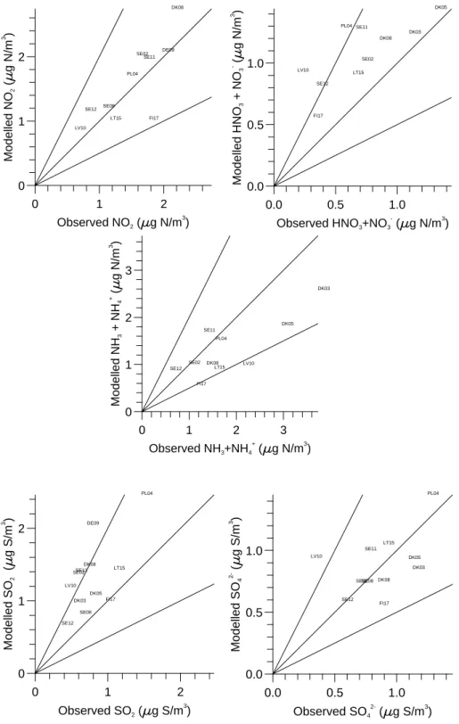
Fig. 1. Comparison between observed
and calculated annual mean concentra-tions in 1999 of nitrogen dioxide, the sum of nitric acid and aerosol phase
ni-trate, and NHx (the sum of NH3 and
NH+4) at the 16 selected stations in
the EMEP programme. The station
codes in the figure are explained in Ap-pendix 1 and straight lines indicate 1:1, 1:2 and 2:1, respectively. 0 1 2 Observed SO2 ( g S/m 3 ) 0 1 2 Modelled SO 2 ( g S/m 3 ) DE09 DK03 DK05 DK08 FI17 LT15 LV10 PL04 SE02 SE08 SE11 SE12 0.0 0.5 1.0 Observed SO4 ( g S/m3) 0.0 0.5 1.0 Modelled SO 4 2- ( g S/m 3 ) DK03 DK05 DK08 FI17 LT15 LV10 PL04 SE02SE08 SE11 SE12
Fig. 2. Comparison between observed
and calculated annual mean concentra-tions in 1999 of sulphur dioxide and sulphate at the 16 selected stations in
the EMEP programme. The station
codes in the figure are explained in Ap-pendix 1 and straight lines indicate 1:1, 1:2 and 2:1, respectively.
between gas phase and aerosol phase e.g. formation of am-monium nitrate from nitric acid and ammonia (see details in Hertel et al., 1995). Cloud processing of gas phase to aerosol
phase compounds e.g. SO2conversion to sulphate, has been
parameterised in a simplified way and is therefore not linked directly to cloud data from Eta (again details may be found in Hertel et al., 1995).
Accounting for horizontal dispersion in Lagrangian mod-els requires analysis of many trajectories, which is highly computer demanding. A parameterisation has therefore been implemented to indirectly account for horizontal dispersion (Hertel et al., 1995). Under ideal conditions a plume grows by 1/10 of the travel distance from a source point (Hanna et al., 1982). The emissions received by the air parcel are
0.0 0.25 0.5 0.75 Observed NO3 conc. prec. (mg N/l) 0.0 0.25 0.5 0.75 Modelled NO 3 - conc. prec. (mg N/l) DE09 DK05 DK08 FI17 FI04 LT15 LV10 PL04 PL05 SE02 SE11 SE12 0.0 0.25 0.5 Observed NH4 + conc. prec. (mg N/l) 0.0 0.25 0.5 Modelled NH 4 + conc. prec. (mg N/l) DE09 DK05 DK08 FI17 FI04 LT15 LV10 PL04 PL05 SE02 SE11 SE12 0 500 1000 Observed Precipitation (mm) 0 500 1000 Modelled Precipitation (mm) DE09 DK05 DK08 FI17 FI04LT15 LV10 PL04 PL05 SE02 SE11 SE12
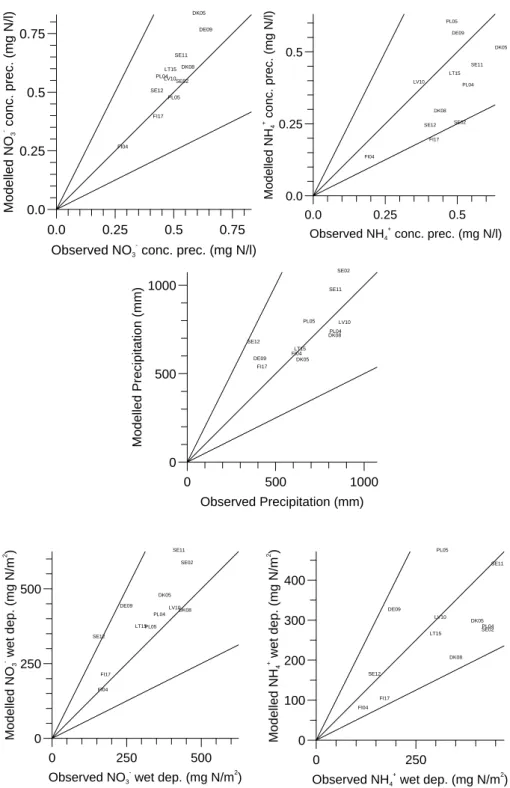
Fig. 3. Comparison between observed
and calculated annual mean nitrate and ammonium concentrations in 1999, and of observed and calculated precipitation at the 16 selected stations in the EMEP programme. The station codes in the figure are explained in Appendix 1 and straight lines indicate 1:1, 1:2 and 2:1, respectively. 0 250 500 Observed NO3 wet dep. (mg N/m2) 0 250 500 Modelled NO 3 - wet dep. (mg N/m 2 ) DE09 DK05 DK08 FI17 FI04 LT15 LV10 PL04 PL05 SE02 SE11 SE12 0 250 Observed NH4 + wet dep. (mg N/m2) 0 100 200 300 400 Modelled NH 4 + wet dep. (mg N/m 2 ) DE09 DK05 DK08 FI17 FI04 LT15 LV10 PL04 PL05 SE02 SE11
SE12 Fig. 4. Comparison between observed
and calculated annual mean wet depo-sition of nitrate and ammonium in 1999 at the 16 selected stations in the EMEP programme. The geographic location of the stations in the figure is given in Ap-pendix 1 and straight lines indicate 1:1, 1:2 and 2:1, respectively.
therefore averaged over an area around the centreline of the trajectory. This area has the width of 1/10 of the remain-ing distance along the trajectory to the receptor point, and thereby horizontal dispersion is indirectly accounted for.
In the operational set up, the ACDEP model uses 96-h back-trajectories. Trajectories are computed from the Eta wind fields and stored with two-hourly steps between posi-tions along the trajectories and for arrival times each 6 h at 00:00, 06:00, 12:00 and 18:00 h. Meteorological parameters for the calculations are provided from the Eta model on
spa-tial resolution of approximately 39 km×39 km and temporal resolution of 1 h. The following meteorological parameters are used: mixed layer wind speed, surface layer wind speed, mixing height, cloud cover, relative humidity, precipitation, surface temperature, mixed layer temperature, surface heat flux and surface momentum. At the beginning of the tra-jectory the model column is given a set of initial concentra-tions. ACDEP was previously initialised with monthly mean background concentrations provide from calculations with the DEM (Zlatev et al., 1992). In this version, however, the
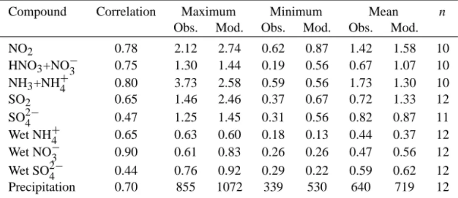
Table 1. Comparison of observed and modelled ambient air concentrations (µg N/m3for the nitrogen compounds and µg S/m3for the sulphur compounds), concentrations in precipitation (µg/l) and precipitation (mm) at the 16 selected EMEP stations situated around the Baltic Sea. Comparisons of annual mean values for the years 1999. The number of stations is indicated by n.
Compound Correlation Maximum Minimum Mean n
Obs. Mod. Obs. Mod. Obs. Mod.
NO2 0.78 2.12 2.74 0.62 0.87 1.42 1.58 10 HNO3+NO−3 0.75 1.30 1.44 0.19 0.56 0.67 1.07 10 NH3+NH+4 0.80 3.73 2.58 0.59 0.56 1.73 1.30 10 SO2 0.65 1.46 2.46 0.37 0.67 0.72 1.33 12 SO2−4 0.47 1.25 1.45 0.31 0.56 0.82 0.87 11 Wet NH+4 0.65 0.63 0.60 0.18 0.13 0.44 0.37 12 Wet NO−3 0.90 0.61 0.83 0.26 0.26 0.47 0.56 12 Wet SO2−4 0.44 0.76 0.92 0.29 0.22 0.59 0.62 12 Precipitation 0.70 855 1072 339 530 640 719 12
initial concentrations are provided on an hourly time resolu-tion from the DEOM model calcularesolu-tions performed within the operational THOR system.
Atmospheric nitrogen and sulphur depositions to Danish land and sea surfaces are calculated with the ACDEP model on routine basis within the Danish National Background Monitoring Programme (DNBMP) (Ellermann et al., 2002). The calculations in DNBMP are performed for 233 receptor points in a 30 km×30 km grid and the results are carefully validated by comparison with measurements from the Dan-ish monitoring stations. In the present work the receptor net from DNBMP has been extended to cover the entire Baltic Sea area. This new receptor net contains in total 690 receptor points. Within the DNBMP the ACDEP model is operated in hind cast mode only, but in the present calculations for the Baltic Sea, the calculations are performed in both hind cast and forecast mode. The forecast computations are performed at 05:00 each day, the results are stored, and selected results are automatically uploaded to an FTP server. Approximately half an hour later they are available at the FTP server for the institutes that will run the marine ecosystem models.
3 Validation of the model
Model results have been compared to measurements from the EMEP monitoring stations around the Baltic Sea. The comparison is performed for 1999 since input data for the ACDEP calculations obtained from the THOR system is available only for the year 1999 and forward, and currently the most recent available monitoring data from EMEP are from 1999. The aim of the performed comparison is to ex-plore the ability of the model to reproduce annual, monthly and diurnal mean values observed in the Baltic Sea area. The comparison is carried out for all relevant wet deposi-tions and ambient air concentradeposi-tions. In the DNBMP the ACDEP model has only been compared to monitoring data
on monthly and annual averages. However, the presented model system aims at producing data with a time resolution sufficient for describing nitrogen inputs on a time scale at which algal blooms take place. Such blooms may build up within a few days (Spokes et al., 1993).
3.1 Annual mean values
The comparison on annual mean basis is shown in Table 1. The comparisons show that the model tends to overestimate annual mean concentrations of nitrogen dioxide (about 10%
in average) and total nitrogen (sum of HNO3 and NO−3)
(about 40% in average), whereas NHx (sum of NH3 and
NH+4) is underestimated (about 20% in average) (see also the
graphical presentation in Fig. 1). The correlation between observed and computed concentrations is, however, in gen-eral reasonably high for all three species (0.78, 0.75 and 0.80, respectively) (Table 1). A good correlation indicates that the spatial distribution of the concentrations is described fairly well.
Sulphate plays an important role in the atmospheric trans-port of ammonium. On average the model reproduces annual sulphate levels reasonably well, but the correlation between modelled and observed sulphate concentrations is relatively poor (0.47) (Table 1). Somewhat better correlation is ob-tained for sulphur dioxide (0.65), but here the concentrations are generally overestimated (see also Fig. 2).
The atmospheric nitrogen input to the North Sea is strongly dominated (about 80% on annual basis) by the
con-tribution from wet deposition (Hertel et al., 2002). The
model comparison shows that nitrate concentrations in pre-cipitation (correlation of 0.90) are well reproduced (Ta-ble 1 and Fig. 3), although there is a tendency for a slight overestimation (in average about 20%). The correlation is smaller but still fairly good for ammonium concentrations in precipitation (0.65), but here with a similar tendency for
JAN MAR MAY JUL SEP NOV 1999 0 1 2 3
Average diurnal mean values
Observed Modelled
NH
3+ NH
4+( g N/m
3)
0 50 Number of points 0.25 0.50 0.75 1.00 1.25 1.50 1.75 2.00 2.25 2.50 2.75 3.00 Observed 0 50 Number of points 0.25 0.50 0.75 1.00 1.25 1.50 1.75 2.00 2.25 2.50 2.75 3.00 ModelledJAN MAR MAY JUL SEP NOV 1999 0.0 0.5 1.0 1.5 2.0
Average diurnal mean values
Observed Modelled
HNO
3+ NO
3( g N/m
3)
0 100 Number of points 0.17 0.33 0.50 0.67 0.83 1.00 1.17 1.33 1.50 1.67 1.83 2.00 Observed 0 50 Number of points 0.17 0.33 0.50 0.67 0.83 1.00 1.17 1.33 1.50 1.67 1.83 2.00 ModelledJAN MAR MAY JUL SEP NOV 1999 0 1 2 3 4
Average diurnal mean values
Observed Modelled
NO
2( g N/m
3)
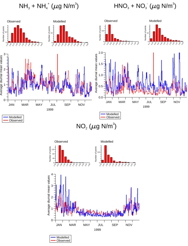
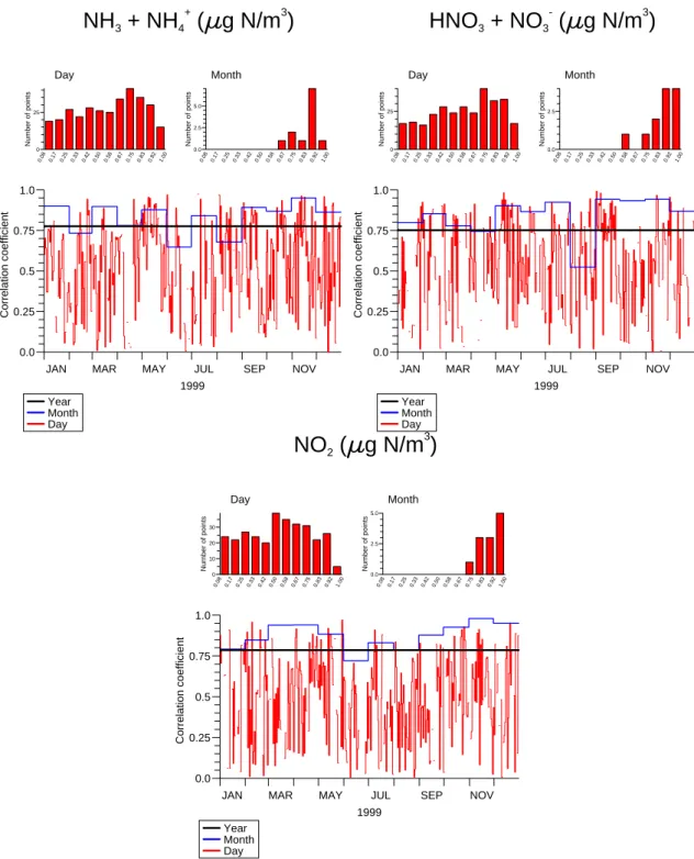
0 40 80 120 Number of points 0.33 0.67 1.00 1.33 1.67 2.00 2.33 2.67 3.00 3.33 3.67 4.00 Observed 0 100 Number of points 0.33 0.67 1.00 1.33 1.67 2.00 2.33 2.67 3.00 3.33 3.67 4.00 ModelledFig. 5. Comparison of average concentrations of NHx(sum of NH3and NH+4), total nitrate (sum of HNO3and NO−3) and NO2for diurnal
mean values – all data for the year 1999. The averaging is performed over the 16 selected EMEP stations for each set of data.
underestimation (in average also about 20%). The same ten-dency is seen for the amount of wet deposition of the two compounds (Fig. 4).
3.2 Analysis of time series
Until now observed and computed annual mean values at the EMEP monitoring stations have been compared. In the fol-lowing we will focus on time series and look into the model performance evaluated for monthly and diurnal mean values.
JAN MAR MAY JUL SEP NOV 1999 0.0 0.25 0.5 0.75 1.0 Correlation coefficient Day Month Year
NH
3+ NH
4 +( g N/m
3)
0 25 Number of points 0.08 0.17 0.25 0.33 0.42 0.50 0.58 0.67 0.75 0.83 0.92 1.00 Day 0.0 2.5 5.0 Number of points 0.08 0.17 0.25 0.33 0.42 0.50 0.58 0.67 0.75 0.83 0.92 1.00 MonthJAN MAR MAY JUL SEP NOV 1999 0.0 0.25 0.5 0.75 1.0 Correlation coefficient Day Month Year
HNO
3+ NO
3( g N/m
3)
0 25 Number of points 0.08 0.17 0.25 0.33 0.42 0.50 0.58 0.67 0.75 0.83 0.92 1.00 Day 0.0 2.5 Number of points 0.08 0.17 0.25 0.33 0.42 0.50 0.58 0.67 0.75 0.83 0.92 1.00 MonthJAN MAR MAY JUL SEP NOV 1999 0.0 0.25 0.5 0.75 1.0 Correlation coefficient Day Month Year
NO
2( g N/m
3)
0 10 20 30 Number of points 0.08 0.17 0.25 0.33 0.42 0.50 0.58 0.67 0.75 0.83 0.92 1.00 Day 0.0 2.5 5.0 Number of points 0.08 0.17 0.25 0.33 0.42 0.50 0.58 0.67 0.75 0.83 0.92 1.00 MonthFig. 6. Correlation coefficients between observed and modelled NHx(sum of NH3and NH+4), total nitrate (sum of HNO3and NO−3) and
NO2for annual, monthly and diurnal mean values – all data for the year1999. The averaging is performed over the 16 selected EMEP
stations for each set of data.
Figure 5 shows observed and modelled diurnal mean concentrations of NHx, total nitrate and nitrogen dioxide
averaged over all available monitoring stations. NHxand
ni-trogen dioxide is generally well reproduced, whereas there is a general tendency to overestimate total nitrate. This result
is in accordance with the comparisons performed on annual mean values for the single stations.
JAN MAR MAY JUL SEP NOV 1999 0.0 2.5 5.0 7.5 10.0
Average diurnal mean values
Observed Modelled
NH
4 +wet dep. (mg N/m
2)
0 100 200 Number of points 0.83 1.67 2.50 3.33 4.17 5.00 5.83 6.67 7.50 8.33 9.17 10.00 Observed 0 100 200 Number of points 0.83 1.67 2.50 3.33 4.17 5.00 5.83 6.67 7.50 8.33 9.17 10.00 ModelledJAN MAR MAY JUL SEP NOV 1999 0.0 2.5 5.0 7.5 10.0
Average diurnal mean values
Observed Modelled
NO
3wet dep. (mg N/m
2)
0 100 Number of points 0.83 1.67 2.50 3.33 4.17 5.00 5.83 6.67 7.50 8.33 9.17 10.00 Observed 0 100 200 Number of points 0.83 1.67 2.50 3.33 4.17 5.00 5.83 6.67 7.50 8.33 9.17 10.00 ModelledJAN MAR MAY JUL SEP NOV 1999
0 5 10 15
Average diurnal mean values
Observed Modelled
Precipitation (mm)
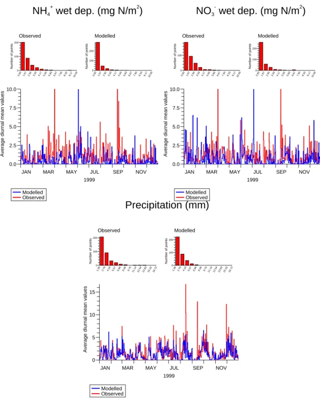
0 100 200 Number of points 1.39 2.79 4.18 5.57 6.96 8.36 9.75 11.14 12.54 13.93 15.32 16.72 Observed 0 100 200 Number of points 1.39 2.79 4.18 5.57 6.96 8.36 9.75 11.14 12.54 13.93 15.32 16.72 ModelledFig. 7. Comparison of average wet depositions of NH+4 and NO−3, and precipitation for diurnal mean values in 1999. The averaging is
performed over the 16 selected EMEP stations for each set of data.
The analysis is expanded to investigate time series of cor-relation coefficients for the spatial distribution performed for the included 16 monitoring stations (see the placement of the stations in Appendix 1). Figure 6 shows the correlation be-tween observed and modelled diurnal mean values, monthly
mean values and the annual mean values. For all three
species reasonably high correlation is obtained for monthly (0.67 to 0.9, 0.56 to 0.9 and 0.75 to 0.9, respectively) and annual mean values (0.77, 0.75 and 0.79, respectively). Al-though some correlation (above 0.5) is obtained for the main part of the time, poor correlation (below 0.4) is frequently obtained when diurnal mean values are evaluated.
JAN MAR MAY JUL SEP NOV 1999 0.0 0.25 0.5 0.75 1.0 Correlation coefficient Day Month Year
NH
4 +conc. prec. (mg N/l)
0 10 Number of points 0.08 0.17 0.25 0.33 0.42 0.50 0.58 0.67 0.75 0.83 0.92 1.00 Day 0 1 2 3 Number of points 0.08 0.17 0.25 0.33 0.42 0.50 0.58 0.67 0.75 0.83 0.92 1.00 MonthJAN MAR MAY JUL SEP NOV 1999 0.0 0.25 0.5 0.75 1.0 Correlation coefficient Day Month Year
NO
3conc. prec. (mg N/l)
0 10 20 Number of points 0.08 0.17 0.25 0.33 0.42 0.50 0.58 0.67 0.75 0.83 0.92 1.00 Day 0 1 2 3 Number of points 0.08 0.17 0.25 0.33 0.42 0.50 0.58 0.67 0.75 0.83 0.92 1.00 MonthJAN MAR MAY JUL SEP NOV 1999 0.0 0.25 0.5 0.75 1.0 Correlation coefficient Day Month Year
Precipitation (mm)
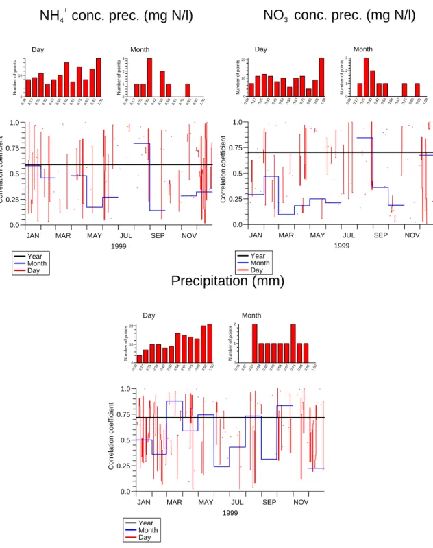
0 10 20 Number of points 0.08 0.17 0.25 0.33 0.42 0.50 0.58 0.67 0.75 0.83 0.92 1.00 Day 0 1 2 Number of points 0.08 0.17 0.25 0.33 0.42 0.50 0.58 0.67 0.75 0.83 0.92 1.00 MonthFig. 8. Correlation coefficients for concentrations in precipitation of NH+4 and NO−3, and precipitation for diurnal mean values for the year
1999. The averaging is performed over the 16 selected EMEP stations for each set of data. The full line represents the correlation coefficients for annual mean values.
The frequency of low nitrate and ammonium concentra-tions in precipitation (<0.17 mg N/l) is higher in the model results than in observations (Fig. 7). For nitrate the total wet deposition is on average somewhat higher than observed due to a few modelled deposition events with high depositions (the plot is not shown here). The precipitation is in
gen-eral well described by the model, although there are some of the observed episodes that are not reproduced. On an-nual basis the modelled and observed ammonium and nitrate wet depositions are fairly correlated (0.58 and 0.71). Already on monthly basis the picture is considerably more scattered and on diurnal basis the results are rather poor (Fig. 8). A
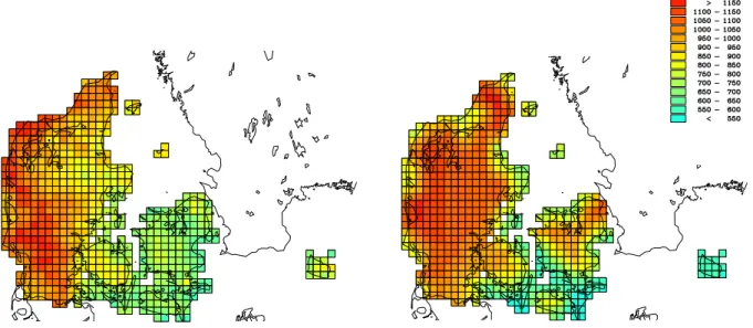
Fig. 9. Gridded annual precipitation on a 10 km×10 km grid from observed precipitation data (left) and obtained from the Eta model (right).
Measurements have been provided by the Danish Meteorological Institute (Scharling, 1998).
significant part of the explanation may be found in the uncer-tainties in precipitation (also shown in Fig. 8). High correla-tions between observacorrela-tions and model results dominate when the annual mean values are evaluated, but even for monthly values a significant part of the results have correlations below 0.4.
3.3 Discussion of model performance
The model still resolves poorly wet depositions on short av-eraging times like diurnal means. It is likely that dry de-positions are similarly uncertain, although a high correlation between observed and modelled ambient air concentrations is generally obtained. Several explanations may be given for this discrepancy of which the most important are believed to be uncertainties in:
– The emission data used for the model calculations, – The precipitation data from the forecast model, – The parameterisation of dry deposition processes, – The parameterisation of aerosol processes,
– Local conditions at the monitoring stations that cannot be resolved by the model, and
– General limitations associated with the principles of the applied Lagrangian model.
Considering emission data, the uncertainties in annual emis-sions on 50 km×50 km EMEP grid have previously been es-timated by EMEP to be in the order of 30 to 40%. However, even though the procedures for the submission of national emission data to the databases are well described, there are still data included in the databases that are subject to future
corrections (Vestreng and Klein, 2002). These uncertain-ties increase further when data are distributed on sub-grid of 16.67 km×16.67 km and especially when highly simplified functions are applied for describing the seasonal and diurnal variation in emissions. Therefore, when variations in diur-nal emissions are the governing factors for the variations in the diurnal concentrations, air pollution models in general will have problems reproducing these values. This is e.g. the case for ammonia in agricultural intensive areas like Den-mark. Thus, we have initiated work that aim at improving the seasonal variation, especially concerning ammonia from agricultural activities.
The operational Eta model at NERI has a horizontal grid
resolution at 0.25×0.25◦, which corresponds to
approxi-mately 39 km over Denmark. A combination of this grid res-olution and the applied version of the Eta step-mountain co-ordinate system with 32 layers have the effect that the Danish land-masses have zero height in the Eta model. Even though Denmark is relatively flat compared to other countries, a not yet published investigation has revealed that a part of the precipitation that falls over Denmark is due to orographic effects. Figure 9 shows a comparison of gridded precipita-tion on 10 km×10 km provided by the Danish Meteorologi-cal Institute and similar figures obtained from the Eta model. The results show that the computed precipitation amounts are within the right order of magnitude, but the model results are more evenly distributed over the Danish land areas compared with the analysed precipitation data. The reason for this dis-crepancy is most probably that the surface topographic de-tails are not sufficiently resolved in the relatively coarse reso-lution in the currently applied version of Eta. However, these issues are subjects of an ongoing project at NERI. The same considerations are expected to be valid for southern Sweden too, however a detailed validation has not been performed.
33
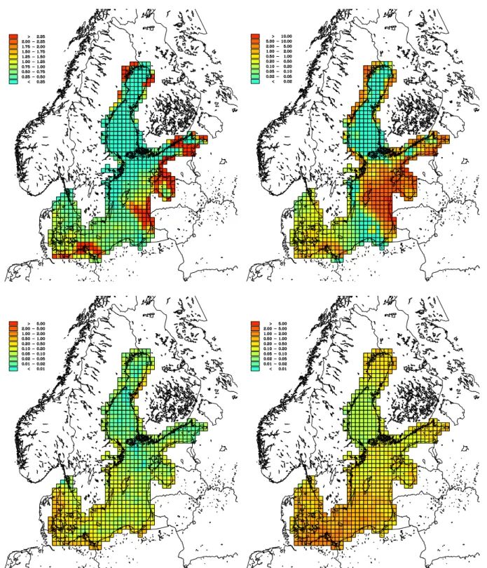
Figure 10. Episode of high nitrogen deposition at the 26th of July 2002. The upper left figure
shows the total nitrogen deposition (tonnes N/km
2) on this day. The upper right figure shows
the precipitation (mm). The lower left figure shows the concentration of ammonia (µg N/m
3)
and the lower right figure the concentration of particulate ammonium (µg N/m
3).
Fig. 10. Episode of high nitrogen deposition on 26 July 2002. The upper left figure shows the total nitrogen deposition (T N/km2) on this
day. The upper right figure shows the precipitation (mm). The lower left figure shows the concentration of ammonia (µg N/m3) and the
lower right figure the concentration of particulate ammonium (µg N/m3).
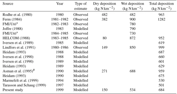
Table 2. Comparison of the present deposition densities to the Baltic Sea with results reported elsewhere.
Source Year Type of Dry deposition Wet deposition Total deposition
estimate (kg N km−2) (kg N km−2) (kg N km−2)
Rodhe et al. (1980) 1980 Observed 482 482 963
Ferm (1984) 1981–1982 Observed 382 900 1282
FMI/Ut¨o∗ 1982–1983 Observed 780
Joffre (1988) 1983 Modelled 790
FMI/Ut¨o∗ 1984–1985 Observed 730
HELCOM (1988) 1983–1985 Observed 80 872 952
Iversen et al. (1989) 1985 Modelled 619
Lindfors et al. (1991) 1980–1986 Observed 149 850 999
Heidam (1993) 1988 Modelled 687
Iversen et al. (1990) 1988 Modelled 660
Iversen et al. (1990) 1989 Modelled 601
Heidam (1993) 1989 Modelled 629
Asman et al. (1995)# 1990 Modelled 271 688 959
Heidam (1993) 1990 Modelled 675
Marmefelt et al. (1999) 1994 Modelled 530
Tarasson and Schaug (1999) 1997 Modelled 501
Present study 1999 Modelled 150 534 684
∗Refered in Lindfors et al. (1991).
#Calculations for Kattegat only.
The current model does not take into account seasonal variation in land cover, and furthermore land use is only strat-ified on sea and land surfaces, where the latter is assumed covered by grass. A detailed land use database is in the pro-cess of being implemented together with surface resistances for various land use types combined with information for the entire model domain (the EMEP area) about growing sea-sons, type of crops etc. The model handles in general aerosol compounds in the same way as gaseous species. When dry deposition is considered, the aerosols are assumed to have a diameter of 0.8 µm. Transformation of gas phase com-pounds to aerosol comcom-pounds is parameterised in a highly simplified way. First order transformation rates are assumed for a number of compounds, whereas formation of e.g. am-monium nitrate is modelled as a function of relative humidity and gas phase concentration of nitric acid and ammonia. A new parameterisation is in process of being implemented. In this parameterisation aerosol size distributions are taken into account, and this is likely to improve the model performance although many parameters need to be determined in this con-text.
The current model version has 6-hourly arrival times for the trajectories, and the points along the trajectories are cal-culated for every 2 h. Thus, it is assumed that using only 6-hourly arrival times at 00:00, 06:00, 12:00, and 18:00 values will produce a reasonable estimate of a diurnal mean value. This may under certain circumstances not be valid. There-fore, a higher time resolution may improve the model per-formance, at the cost of an increase in computer calculation
time. However, the present model set up is limited by the fact that the results of the calculations must be available at 06:00 each morning from the THOR system. Depositions are interpolated between arrival times, which especially for wet depositions may lead to considerable errors. The movement of the air column along the trajectory is also computed from interpolation between the calculated 2-hourly points. Close to arrival at the receptor point this may lead to uncertainties in the received emissions.
The wet deposition processes are parameterised using a commonly applied method. However, a more precise way to compute wet depositions could be obtained by implement-ing physical and chemical cloud droplet processes directly. However, this requires a full 3-D model that includes both meteorological processes and air pollution processes in one coupled system. The clear disadvantage of such a system is the tremendous computer resource demand, which means that this type of model usually is applied for studying only short time periods (Carmichael et al., 1991; von Salzen and Schl¨unzen, 1999; Kim and Cho, 1999; Hogrefe et al., 2001). The mainly coastal monitoring stations used in the anal-ysis of the model performance may in some cases be influ-enced by very local conditions that cannot be resolved in the current version of the model system. One example is the gen-eration of sea breeze circulation cells that is not resolved in the meteorological data from the Eta model in the present application, and thus cannot be reflected in the computed nitrogen depositions either. Another issue regarding the com-parison of calculations and observations is that the model
Fig. 11. Calculated nitrogen deposition (T N km−2) to the entire Baltic Sea in 1999.
represents an average condition over a certain area (in this case 30 km×30 km), whereas the observations reflect the lo-cal conditions at a specific point. This may especially affect the wet depositions, since the precipitation amount may vary up to a factor of five or more within few kilometres. In some cases a specific rain event may pass close by the monitoring station, but without contributing at all to what is collected in the bulk sampler.
The Lagrangian model type has the advantage to have rel-atively low computer demands, especially when a limited number of receptor points are considered. Furthermore the model scale may be changed along the trajectory, e.g. allow-ing for higher resolution in input data when the air parcel is approaching the receptor point. However, the uncertainty in the description of the transport may be significant in this type of models, especially considering the first part of the 96 h back-trajectory. Furthermore, wind turning with height is disregarded in the model, which may be a rather crude as-sumption. The next generation of nitrogen deposition model at NERI will therefore be a nested grid 3-dimensional Eule-rian model with high spatial and temporal resolution (Frohn et al., 2001; 2002). 0 100 200 300 Day of year 0 50 100 150 Deposition kg N/km 2 1 2 3 4 5 6 7 8 9 10 11 12 13 14 15 16 17 18 19 20 21 22 23 24 25 26 27 28 29 30 31 32 33 34 35 36 37 38 39 40 41 42 43 44 45 46 47 48 49 50 51 52 53 54 55 56 57 58 59 60 61 62 63 64 65 66 67 68 69 70 71 72 73 74 75 76 77 78 79 80 81 82 83 84 85 86 87 88 89 90 91 92 93 94 95 96 97 98 99 100 101 102 103 104 105 106 107 108 109 110 111 112 113 114 115 116 117 118 119 120 121 122 123 124 125 126 127 128 129 130 131 132 133 134 135 136 137 138 139 140 141 142 143 144 145 146 147 148 149 150 151 152 153 154 155 156 157 158 159 160 161 162 163 164 165 166 167 168 169 170 171 172 173 174 175 176 177178 179 180 181 182 183 184 185 186 187 188 189 190 191 192 193 194 195 196 197 198 199 200 201 202 203 204 205 206 207 208 209 210 211 212 213 214 215 216 217 218 219 220 221 222 223 224 225 226 227 228 229 230 231 232 233 234 235 236 237 238 239 240 241 242 243 244 245 246 247 248 249 250 251 252 253 254 255 256 257 258 259 260 261 262 263 264 265 266 267 268 269 270 271 272 273 274 275 276 277 278 279 280 281 282 283 284 285 286 287 288 289 290 291 292 293 294 295 296 297 298 299 300 301302 303 304 305 306 307 308 309 310 311 312 313 314 315 316 317 318 319 320 321 322 323 324 325 326 327 328 329 330 331 332 333 334 335 336 337 338 339 340 341 342 343 344 345 346 347 348 349 350 351 352 353 354 355 356 357 358 359 360 361 362 363 364 365 366 367 368 369 370 371 372 373 374 375 376 377 378 379 380 381 382 383 384 385 386 387 388 389 390 391 392 393 394 395 396 397 398 399 400 401 402 403 404 405 406 407 408 409 410 411 412 413 414 415 416 417 418 419 420 421 422 423 424 425 426 427 428 429 430 431 432 433 434 435 436 437 438 439 440 441 442 443 444 445 446 447 448 449 450 451 452 453 454 455 456 457 458 459 460 461 462 463 464 465 466 467 468 469 470 471 472 473 474 475 476 477 478 479 480 481 482 483 484 485 486 487 488 489 490 491 492 493 494 495 496 497 498 499 500 501 502 503 504 505 506 507 508 509 510 511 512 513 514 515 516 517 518 519 520 521 522 523 524 525 526 527 528 529 530 531 532 533 534 535 536 537 538 539 540 541 542 543 544 545 546 547 548 549 550 551 552 553 554 555 556 557 558 559 560 561 562 563 564 565 566 567 568 569 570 571 572 573 574 575 576 577 578 579 580 581 582 583 584 585 586 587 588 589 590 591 592 593 594 595 596 597 598 599 600 601 602 603 604 605 606 607 608 609 610 611 612 613 614 615 616 617 618 619 620 621 622 623 624 625 626 627 628 629 630 631 632 633 634 635 636 637 638 639 640 641 642 643 644 645 646 647 648 649 650 651 652 653 654 655 656 657 658 659 660 661 662 663 664 665 666 667 668 669 670 671 672 673 674 675 676 677 678 679 680 681 682 683 684 685 686 687 688 689 690
Fig. 12. Calculated maximum diurnal nitrogen deposition density
(kg N km−2) to 690 receptor points distributed over the entire Baltic
Sea in 1999. The numbers in the plot refer to the receptor grid number, which starts in the most northern part of the Baltic and ends with the Danish waters. Red colour indicates Botvian Sea and Botvian Bay, blue indicate Gulf of Finland, orange indicate Gulf of Riga, yellow-green indicate Baltic proper (exclusive Danish waters) and dark green indicate Danish waters.
4 Nitrogen depositions to the Baltic Sea
The performed model calculations show a total nitrogen de-position in the year 1999 to the entire Baltic Sea of about
317.8 kT N to an area of 464 406 km2. This may be compared
with model results and measurements from other sources. Model calculations performed with the Swedish MATCH model gave a considerably lower value of 220 kT N for the year 1994 (Marmefelt et al., 1999) and EMEP model results have shown values of 285.4; 261.2 and 280.3 kT N for the years 1988, 1989 and 1990, respectively (Heidam, 1993). However, both the MATCH model study and EMEP report
an area for the Baltic Sea on only 415 000 km2. Up
scal-ing to an area of 464 406 km2, the EMEP estimates show
318.7, 291.8 and 313.0 kT N for 1988, 1989 and 1990, re-spectively. A more recent estimate from EMEP says 208 kT N for 1997 (Tarras´on and Schaug, 1999), which up scaled to the area used in the present study is equal to 233 kT. The most recent value from EMEP is considerably lower (about 27%) than the present finding, whereas the older EMEP val-ues in general are in good agreement with the present esti-mate. After a similar up scaling, however, the result from the MATCH model calculations is also considerably lower (23% lower) than the results from the present study – up scaled the MATCH model result gives 246 kT N. The model results
Table A1. Code of the monitoring stations used in the model validation. The code is given together with the name of the site, geographic
coordinates and altitude above sea level. The geographic location of the stations is shown in Fig. A1.
Site Code Geographic coordinates Altitude above sea level (m)
Country: Denmark Tange DK03 56◦210N, 9◦360E 13 Keldsnor DK05 54◦440N, 10◦440E 9 Anholt DK08 56◦430N, 11◦310E 40 Country: Finland ¨ Aht¨ari FI04 62◦330N, 24◦130E 4 Virolahti II FI17 60◦310N, 27◦410E 4 Country: Lithuania Preila LT15 (SU15) 55◦210N, 21◦040E 5 Country: Latvia Rucava LV10 (SU10) 56◦130N, 21◦130E 18 Country: Poland Leba PL04 54◦450N, 17◦320E 2 Diabla Gora PL05 54◦090N, 22◦040E 157 Country: Sweden R¨orvik SE02 57◦250N, 11◦560E 10 Hoburg SE08 56◦550N, 18◦090E 58 Vavihill SE11 56◦010N, 13◦090E 172 Aspvreten SE12 58◦480N, 17◦230E 20 Country: Estonia
Lahemaa EE09 (SU09) 59◦300N, 25◦540E 32
Vilsandi EE11 (SU11) 58◦230N, 21◦490E 6
Country: Germany
Zingst DE09 54◦260N, 12◦440E 1
in the present study gives an average deposition for 1999 of
about 684 kg N km−2of which wet deposition accounts for
about 78%. It should be noted that at least for Danish marine waters 1997 was a relatively dry year compared with 1999, and this may explain a considerable part of the differences in the estimates. Ellermann et al. (2002) reported a precipita-tion of 520 mm in 1997 and 780 in 1999 at the island Anholt in the middle of the Kattegat Strait. Furthermore, years with low precipitation also have a low net nitrogen deposition and years with high precipitation are years with high total nitro-gen deposition (Ellermann et al., 2002). Reported studies on atmospheric nitrogen deposition to the Baltic in general show a contribution from wet deposition on the order of 70–80% (Table 2), which is in very good agreement with the present results. The reported studies show depositions in the range
600 to 1300 kg N km−2, where the highest values refer to the
1980’ties. Taking into account that concentrations of aerosol bound nitrogen compounds have decreased some 30% over
that time period, the present results are in good agreement with previous studies, since the highest values are reported for the 1980’ties and early 1990’ties.
Episodes of high atmospheric nitrogen deposition are solely the result of precipitation events. Depositions may be somewhat elevated close to the coast when transport from nearby agricultural activities lead to high ammonia concen-trations. However, the resulting dry deposition is consider-ably smaller than what is observed from rain out of aerosol phase ammonium and nitrate. Figure 10 shows the simu-lation of an event with high local wet deposition of atmo-spheric nitrogen in a belt from the coast of Poland and out to Gotland in the Baltic Sea. When the different plots are com-pared it is clear that the high deposition appears where there is an overlap between high aerosol phase concentrations and high precipitation amounts.
The computed total atmospheric nitrogen deposition to the Baltic Sea in 1999 is shown in Fig. 11. The deposition has
DK03 DK05 DK08 FI04 FI17 LT15 LV10 PL04 PL05 SE02 SE08 SE11 SE12 EE09 EE11 DE09
Fig. A1. Geographic location of the monitoring stations used in the
model validation. The names of the sites, the geographic coordi-nates and the altitude above sea level are given in Table A1.
a pronounced south–north gradient with depositions in the
range about 1000 kg N km−2 in south and 200 kg N km−2
in north. This gradient is due to transport from the areas with high emission density in the northern part of the Euro-pean continent. Tarras´on and Schaug (1999) reported below
100 kg N km−2in the north and between 400 and 700 in the
south, but again it should be noted that these values related to 1997, where precipitation about over Danish waters were considerably lower than in 1999.
According to the model results for episodes, the maximum diurnal depositions over the Danish waters took place in the mid summer period where the algae growth is high (Fig. 12). For the northern part of the Baltic maximum values were distributed over most of the year. These results are again strongly dependent on the prediction of precipitation events and therefore rather uncertain.
5 Conclusions
The aim of the evaluation of the model performance was here to investigate how well the model reproduces air concentra-tions and wet deposiconcentra-tions when short averaging times are considered. The analysis has shown that the model repro-duces reasonably well annual and monthly mean ambient air
concentrations. Diurnal mean concentrations of NHx(sum of
NH3and NH+4) and NO2are fairly well reproduced, whereas
total nitrate (sum of HNO3and NO−3) is somewhat
overesti-mated by the model. Wet depositions of nitrate and ammonia are fairly well described for annual mean values, whereas the uncertainty is high for the monthly mean values and the wet deposition is poorly described for diurnal mean values. The model calculations show that annual nitrogen depositions to
the Baltic are in the range from 1000 kg N km−2in the south
to 200 kg N km−2in the north, with an overall load of 318 kT
N in 1999 to an area of 464 406 km2. The present finding of
the overall load is somewhat higher than what is found in literature, but this may be partly due to differences between years. The present result is for the year 1999, where high precipitation amounts are reported for the Danish marine wa-ters, whereas literature values all refer to years before 1998. Maximum diurnal depositions in 1999 seem to appear in the summer period for the Danish waters, but seem also to ap-pear at any time of year for the rest of the Baltic. This result is quite uncertain and may only apply to this specific year.
Appendix A: Monitoring stations used in the model vali-dation
The following EMEP monitoring stations were included in the model validation for the year 1999 (further information may be obtained from http://www.nilu.no/projects/ccc/index. html). The station codes in Table A1 are used in several of the plots and the geographic location of the stations is shown in Fig. A1.
Acknowledgements. The Nordic Council of Ministers funded the presented work as part of the project 00/01 NO COMMENTS (http:
//www.imr.no/∼morten/nocomments/). Measurements from EMEP
monitoring stations around the Baltic Sea in 1999 have been ob-tained from the web at the Norwegian Institute for Air Research (http://www.nilu.no/projects/ccc/emepdata.html). S. Reis and U. Schwarz, University of Stuttgart provided detailed emission data from the EUROTRAC GENEMIS project for the EU countries.
References
Asman, W. A. H., Berkowicz, R., Christensen, J., Hertel, O., and Runge, E. H.: Atmospheric Contribution of nitrogen species
to Kattegat (In Danish: Atmosfærisk tilførsel af
kvælstof-forbindelser til Kattegat). Under the Series “Marine Research from the Danish Environmental Protection Agency”, No. 37, Danish Environmental Protection Agency, Copenhagen, Den-mark, 1994.
Asman, W. A. H., Hertel, O., Berkowicz, R., Christensen, J., Runge, E.H., Sørensen, L. L., Granby, K., Nielsen, H., Jensen, B., Gryn-ing, S. E., Sempreviva, A. M., Larsen, S., Hummelshøj, P., Jensen, N. O., Allerup, P., Jørgensen, J., Madsen, H., Overgaard, S., and Vejen, F.: Atmospheric Nitrogen Input to the Kattegat Strait, Ophelia, 42, 5–28, 1995.
Ambelas Skjøth, C., Hertel, O., and Ellermann, T.: Use of a Trajec-tory Model in the Danish nation-wide background Programme, Phys. Chem. Earth., 27, 35, 1469–1477, 2002.
Berkowicz, R., Hertel, O., Sørensen, N. N., and Michelsen, J. A.: Modelling Air Pollution from Traffic in Urban Areas, in proceed-ings from IMA meeting on “Flow and Dispersion Through Ob-stacles”, Cambridge, England, 28 to 30 March, 1994, edited by Perkins, R. J. and Belcher, S. E., 121–142, 1997.
Berkowicz, R.: A simple model for urban background pollution, Environmental Monitoring and Assessment, 65, 259–267, 2000a. Berkowicz, R.: OSPM – a parameterised street pollution model, En-vironmental Monitoring and Assessment, 65, 323–331, 2000b. Brandt, J., Christensen, J. H., Frohn, L., Berkowicz, R., and
Palm-gren, F.: The DMU-ATMI THOR air pollution forecast system system description. Technical Report from NERI No. 321, Na-tional Environmental Research Institute, PO Box 358, Frederiks-borgvej 399, DK-4000 Roskilde, Denmark, 60, http://www.dmu. dk/1 viden/2 Publikationer/3 fagrapporter/default.asp 2000. Brandt, J., Christensen, J. H., Frohn, J. M., Palmgren, F.,
Berkow-icz, R., and Zlatev, Z.: Operational air pollution forecasts from European to local scale, Atmos. Environ., 35, 1, S91–S98, 2001a. Brandt, J., Christensen, J. H., Frohn, L. M., and Berkowicz, R.: Operational air pollution forecast from regional scale to urban street scale, Part 1: system description, Physics and Chemistry of the Earth (B), 26, 10, 781–786, 2001b.
Brandt, J., Christensen, J. H., and Frohn, L. M.: Operational air pollution forecast from regional scale to urban street scale. Part 2: performance evaluation, Physics and Chemistry of the Earth (B), 26, 10, 825–830, 2001c.
Brutsaert, W. H.: Evaporation into the Atmosphere, Reidel, Boston, 1982.
Carmichael, G. R., Peters, L. K., and Saylor, R. D.: The STEM-II regional scale acid deposition and photochemical oxidant model 1 and overview of model development and applications, Atmo-spheric Environment Part A – General Topics, 25, 10, 2077– 2090, 1991.
Ellermann, T., Hertel, O., Munies, C., and Kemp, K.: NOVA
2003, Atmospheric Deposition 2001 (In Danish: NOVA
2003, Atmosfrisk deposition 2001), Danish National
En-vironmental Research Institute, PO Box 358,
Frederiks-borgvej 399, 4000 Roskilde, Denmark, Technical Report, 418, 82, http://www.dmu.dk/1 viden/2 Publikationer/3 fagrapporter/ rapporter/FR418.pdf, 2002.
EMEP, Estimates of airborne transboundary transport of sulphur and nitrogen over Europe, EMEP/MSC-W Report 1/88, Oslo, Norway, 79, 1988.
Frohn, L. M., Christensen, J. H., and Brandt, J.: Development of a regional high resolution air pollution model – The numerical approach, J. Comp. Phys., 179, 68–92, 2002.
Frohn, L. M., Christensen, J.H., Brandt, J., and Hertel, O.: Devel-opment of a high resolution integrated nested model for studying air pollution in Denmark, Physics and Chemistry of the Earth (B), 26, 10, 769–774, 2001.
Gery, M. W., Whitten, G. Z., and Killus, J. P.: Development and testing of the CBM-IV for urban and regional modeling. EPA-600/3-88-012 US EPA, Research Triangle Park, N.C., 1989a. Gery, M. W., Whitten, G. Z., Killus, J. P., and Dodge, M. C.:
A photochemical kinetics mechanism for urban and regional scale computer modeling, J. Geophys. Res., 94D, 12 925–12 956, 1989b.
Hanna, S. R., Briggs, G. A., and Hosker Jr., R. P.: Handbook on Atmospheric Diffusion, Technical Information Center, U.S.
De-partment of Energy, 102, 1982.
Heidam, N. Z.: Nitrogen deposition to the Baltic Sea: Experimental and model estimates, Atmos. Environ., 27A, 6, 815–822, 1993. HELCOM: Baltic Marine Environment Protection Commission:
deposition estimates to the Baltic Sea area based on reported data for 1983–1985 edited by S¨oderlund, R. and Areskoug, H., Reprints Copy, 25, 1988.
Hertel, O., Berkowicz, R., Christensen, J., and Hov, Ø.: Tests of two Numerical Schemes for use in Atmospheric Transport-Chemistry models, Atmos. Environ., 27A, 16, 2591–2611, 1993.
Hertel, O., Christensen, J., Runge, E. H., Asman, W. A. H., Berkow-icz, R., Hovmand, M. F., and Hov, Ø.: Development and Testing of a new Variable Scale Air Pollution Model – ACDEP, Atmos. Environ., 29, 11, 1267–1290, 1995.
Hertel, O., Ambelas Skjøth, C., Frohn, L. M., Vignati, E., Fryden-dall, J., de Leeuw, G., Swarz, S., and Reis, S.: Assessment of the Atmospheric Nitrogen and sulphur Inputs into the North Sea us-ing a Lagrangian model, Phys. Chem. Earth, 27, 35), 1507–1515, 2002.
Hogrefe, C., Rao, S. T., Kasibhatla, P., Hao, W., Sistla, G., Mathur, R., and McHenry, J.: Evaluating the performance of regional.scale photochemical modeling system: Part II – ozone predictions, Atmos. Environ., 35, 24, 4175–4188, 2001. Huang, H-C. and Chang, J.: On the performance of numerical
solvers for a chemistry submodel in three-dimensional air quality models, I. Box model simulations, J. Geophys. Res., 106, D17, 20 175–20 188, 2001.
Iversen, T., Saltbones, J., Sandnes, H., Eliasen, A., and Hov, Ø.: Airborne transboundary transport of sulphur and nitrogen over Europe – Model description and calculations, EMEP MSC-W Report 2/89, 92, 1989.
Iversen, T., Halvorsen, N. E., Saltbones, J., and Sandnes, H.: calcu-lated budgets for airborne sulphur and nitrogen in Europe, EMEP MSC-W Report 2/90, 142, 1990.
Joffre, S.: Parameterisation and assessment of processes affecting the long-range transport of airborne pollutants to the sea, Finnish Meteorological Institute Contribution No. 1, 49, 1988.
Kim, J. and Cho, S. Y.: Application of the nested grid STEM to an early summer acid rain in South Korea, Atmos. Environ., 33, 19, 3167–3181, 1999.
Larsson, U., Elmgren, R., and Wulff, F.: Eutrophication and the Baltic Sea, Causes and consequences, Ambio, 14, 9–14, 1985. Lindfors, V., Joffre, S. M., and Damski, J.: Determination of the
wet and dry deposition of sulphur and nitrogen conpounds over the Baltic Sea using actual meteorological data, Finish Meteo-rological Institute Contributions No. 4, Helsinki, Finland, 111, 1991.
Lindfors, V., Joffre, S., and Damski, J.: Meteorological variability of the wet and dry deposition of sulphur and nitrogen compounds over the Baltic Sea, Water, Air, and Soil Pollution, 66, 1–28, 1993.
Marmefelt, E., Arheimer, B., and Langner, J.: An integrated biogeo-chemical model system for the Baltic Sea, Hydrobiologia, 393, 45–56, 1999.
Meyer-Reil, L.-A., and K¨oster, M.: Eutrophication of Marine Wa-ters: Effects on Benthic Microbial Communities, Marine Pollu-tion Bulletin, 41, 1–6,, 255, 263, 2000.
Møhlenberg, F.: Effects of meteorology and nutrient load on oxygen depletion in a Danish micro-tidal estuary, Aquatic Ecology, 33,
55–64, 1999.
Nickovic, S., Michailovic, D., Rajkovic, B., and Papdopulus, A.: The weather Forecasting System SKIRON II, Description of the model, June, Athens, 228, 1998.
Paerl, H. W.: Coastal eutrophication in relation to atmospheric de-position: current perspectives, Ophelia, 41, 237–259, 1995. Rodhe, H., S¨oderlund, R., and Ekstedt, J.: Deposition of airborne
pollutants on the Baltic, Ambio, 9, 3:4, 168–173, 1980. Sandnes, H.: Calculated budgets for airborne acidifying
compo-nents in Europe, 1985, 1987, 1988, 1989, 1990, 1991 and 1992, EMEP MSC-W Report 1/93, Norwegian Meteorological Insti-tute, PO Box 43, N-0313, Oslo, Norway, 1993.
Scharling, M.: Climatic grit Denmark, Precipitation 10 km×10 km, Description of Methods, in Danish: Klimagrid Danmark, Nedbør 10 km×10 km, Metodebeskrivelse), Danish Meteorological In-stitute, Ministry of Transport, Copenhagen, Technical Report 98-17, 16, 1998.
Slinn, S. A. and Slinn, W. G. B.: Predictions for particle deposition on natural waters, Atmos. Environ., 14, 1013–1016, 1980. Spokes, L., Jickells, T., Rendell, A., Schulz, M., Rebers, A.,
Dan-necker, W., Kr¨uger, O., Lermakers, M., and Baeyens, W.: High Atmospheric Nitrogen Deposition Events Over the North Sea, Marine Pollution Bulletin, 26, 12, 698–703, 1993.
Spokes, L., Yeatman, S. G., Cornell, S. E., and Jickells, T.: Nitro-gen deposition to the eastern Atlantic Ocean, The importance of south-easterly flow, Tellus, 52B, 37–49, 2000.
Tarras´on, L. and Schaug, J. (Eds.): Transboundary acid deposition in Europe, EMEP summary Report 1999, Norwegian Meteoro-logical Institute Research Report No. 83, 70, 1999.
Tilmes, S., Brandt, J., Flatøy, F., Bergstr¨om, R., Flemming, J., Langner, J., Christensen, J. H., Frohn, L. M., Hov, Ø., Jacob-sen, I., Reimer, E., Stern, R., and Zimmermann, J.: Comparison of five Eulerian ozone prediction systems for summer 1999 us-ing the German monitorus-ing data, J. Atmos. Chem., 42, 91–121, 2002.
Richardson, K.: Harmful or exceptional Phytoplankton Blooms in the Marine Ecosystem, Advances in marine biology, 31, 301– 385, 1997.
Rosenberg, R., Elmgren, R., Fleischer, S., Jonsson, P., Persson, G., and Dahlin, H.: Marine eutrophication case studies in Sweden, Ambio, 19, 102–108, 1990.
Rydberg, L., Edler, L., Floderus, S., and Gran´ell, W.: Interaction Between Supply of Nutrients, Primary Production, Sedimenta-tion and Oxygen ConsumpSedimenta-tion in the SE Kattegat, Ambio, 19, 3, 134–141, 1990.
Vestreng, V. and Klein, H.: Emission data reported to
UN-ECE/EMEP: Quality assurance and trend analysis & presenta-tion on WebDab. EMEP MSC-W Status report, EMEP/MSC-W Note 1, 2002.
Von Salzen, K. and Schl¨unzen, H.: Simulation of the dynamics and composition of secondary and marine inorganic aerosols in the coastal atmosphere, J. Geophys. Res., 104, D23, 30 201–30 217, 1999.
Wesely, M. L. and Hicks, B. B.: Some factors that affects the deposition of sulphur dioxide and similar gases on vegetation, JAPCA, 27, 1110–1116, 1977.
Zlatev, Z., Christensen, J., and Hov, Ø.: A Eulerian air pollution model for Europe with nonlinear chemistry, J. Atmos. Chem., 15, 1–37, 1992.